(include assigned division number from I to X) `
QUANTIFICATION AND CONSEQUENCES OF CONSERVATISM IN
EQUIPMENT FUNCTIONAL FRAGILITY EVALUATION
Bradley T. Yagla1, Eddie M. Guerra2, Enrique Bazan-Zurita3, and Lawrence A. Mangan4
1
Engineering Associate, RIZZO Associates, USA
2
Senior Project Engineer, RIZZO Associates, USA
3Chief Engineer, RIZZO Associates, USA
4
Senior Nuclear Engineer, FirstEnergy Nuclear Operating Company, USA
ABSTRACT
The conservativeness in Seismic Probabilistic Risk Assessments does not only constitute a current industry debate but could drive economic feasibility for such projects. There is consensus that realistic, unbiased, demand and capacity parameters must be used in the assessment. The fragility analysis step of the process develops quantitative capacities, or fragilities, for structures, systems and components identified as potential contributors to plant risk. Functional fragilities are usually established based on earthquake experience, generic testing, or component specific testing. In general, testing provides the most realistic measure of capacity. However, seismic test reports may be limited or unavailable for a component and the analyst has to rely on generic equipment ruggedness spectra (GERS). GERS were developed for screening purposes in the A-46 program and Seismic Margin Assessments, and their calculation with a conservative bias was acceptable. However, conservatism in SPRA results may mask the true contribution to risk of critical equipment thus underscoring the importance to avoid or at least limit conservatism in fragility estimates. In this study we adopt a Bayesian approach to enhance GERS for two particular equipment categories with available data from additional test reports for similar components. Test reports contain both survival and failure information; therefore we propose an approach for consistent interpretation of the data. The enhanced GERS can be used to calculate more realistic fragilities for components lacking specific seismic test reports. The results of this study can also serve to improve functional fragility increase factors for the selected equipment category with their corresponding uncertainty, for use in risk quantification studies. Clearly, plant seismic risk is sensitive to conservatism in functional fragility data such as GERS for critical components and insensitive for rugged or non-critical components. The studies presented herein could be useful to both fragility analysts and PRA managers who must address challenges associated with conservativeness in SPRA.
INTRODUCTION
Ideally, functional fragility of equipment in NPPs is based on component-specific testing performed for a high demand response spectrum (i.e. near or over the component limit capacity), especially for risk-significant components. However, adequate test data may not be available for some components and generic information is relied upon to estimate functional fragilities. Two widely used generic methods are earthquake experience data from EPRI (2009 and 1991a) and generic testing data from EPRI (1991b).
GERS were developed for individual equipment categories based on several shake table tests. Both survival and failure data were recorded during the tests. The upper envelope of the survivals and the lower envelope of the failures were considered in defining the GERS.
Both the reference spectrum and the GERS were developed for screening purposes in the A-46 program and Seismic Margin Assessments. A conservative bias was acceptable within such a context. However, because fragility inputs to SPRA are required to be realistic and unbiased, it is of interest to reduce, and preferably eliminate, the conservatism in functional fragility data. It is noted that conservatively biased estimates of the capacity of one component could mask the weakness of other components, which have been more realistically evaluated. In this paper, we propose the use of Bayesian statistical concepts for an unbiased incorporation of all sources of information in the estimation of fragilities, attempting to minimize undesired conservatism.
Implementation of Bayesian concepts in SPRA fragility calculation are reported by EPRI (2014). The technical report focuses on Bayesian updating of the earthquake experience database. The fundamentals
of Bayes’ Rule are followed in EPRI (2014) and within this paper; however, there are differences in the methodology and application.
BAYES’ RULE BACKGROUND
An inherent challenge in probabilistic studies is dealing with an unknown value, or state of nature, of a parameter. When limited data are available, estimates of the true value of the parameter may have a weak basis. However, any available prior knowledge of the parameter can be combined with experimental
observations according to Bayes’ rule to strengthen the estimated value of the parameter via a posterior
probability distribution per Benjamin and Cornell (1970). Furthermore, the use of conjugate priors allows for a convenient relationship between prior and posterior distributions, because both distributions have the same functional form. For example, when the prior distribution is normally distributed, then the posterior distribution, which incorporates the likelihood of the data, also becomes normally distributed. For this case, the parameters defining the prior distribution, sample likelihood function and posterior distribution are presented in following subsections.
Prior Distribution
The prior distribution can be described by a subjective opinion or by previously existing data or estimates. The parameters defining the distribution: n′, `
x′, and s′ represent the equivalent prior sample size, prior
sample mean and the prior sample standard deviation, respectively. These parameters are considered tobe the “known.”
Sample Likelihood Function
The sample likelihood function can be developed by statistical analysis based on the prior distribution and on a data set, and n, `x, and s, represent the size, mean and standard deviation, respectively, of the
sample.
Posterior Distribution
For a normally distributed variable, given the prior distribution and sample data, the Bayesian analysis develops the three parameters of the updated posterior distribution, are given by equations (1) through (3).
n′′ is the posterior distribution effective sample size
݊
ᇱᇱݔԢԢ ൌ ݊ݔ ݊ԢݔԢ
(2)`x′′ is the mean of the posterior distribution
ሺ݊
ᇱᇱെ ͳሻݏ
ᇱᇱଶ ݊
ᇱᇱݔ
ᇱᇱଶൌ ൣሺ݊ െ ͳሻݏ
ଶ ݊ݔ
ଶ൧ ൣሺ݊
ᇱെ ͳሻݏ
ᇱଶ ݊
ᇱݔԢ
ଶ൧
(3)s′′ is the standard deviation of the posterior distribution sample
Working in the logarithmic space, the conjugate property of the normal distribution can be conveniently transferred to a lognormally distributed variable.
CONSISTENT INTERPRETATION OF NON-FAILURE INFORMATION
Two basic types of data on the seismic capacity of a given type of component can be acquired from laboratory testing or observations after actual earthquakes. The first type reports cases where failures occurred at given input accelerations and constitute direct measures of capacity. Values of the second type are input (laboratory or actual) accelerations for which failure did not occur and only indicate that the capacity is at least the input acceleration. Sometimes, entries of the second type are conservatively taken as corresponding to failures.
Data points corresponding to observed failures do not require any modification and the reported capacity was taken as the input demand that triggered failure. For a consistent incorporation of the second type of
data, we developed “interpreted” failure capacities when the specimens performed their intended
functions before, during and after their tests. Clearly, the failure capacities are higher than the maximum recorded input demands, v. Thus, failure would occur above v, in accordance with the prior distribution, fx(), of the capacity as illustrated by the shaded area in Figure 1. Normalized to have a value of unity, the
shaded area constitutes the probability distribution of the capacity, fCx(), conditional to the observed
survival. The likelihood of the failure happening at exactly the value w≥ v is fCx(w) dx. Thus, the mean
Figure 1. Interpretation of Non-Failure Information.
POSTERIOR BAYESIAN FRAGILITY
The following scenario illustrates our proposed derivation of updated functional fragilities for particular equipment. The GERS is taken as the initial basis for functional fragility as long as the equipment met the applicable caveats. Let us now consider that test reports are available for similar equipment which were not used in the development of the GERS. A realistic probabilistic assessment must account for the
two sources of information: the existing -a priori- knowledge embodied in the GERS, and the additional
experimental data, to develop updated (posteriori) statistical parameters. To this end, we carry out the following procedure:
1) Select equipment category.
2) Obtain GERS from EPRI (1991b) and corresponding median capacity increase factors and variability
from EPRI (1994) for equipment category of interest.
3) Obtain and examine test reports for equipment similar to those included in generic testing class
represented by GERS.
4) Identify response spectra (TRS) from test reports and record test and specimen information.
5) Standardize TRS to consistent frequency points, damping, and clipping.
6) Select spectral acceleration in representative frequency range from standardized TRS.
7) Obtain sample statistics using consistent interpretation of non-failure data.
8) Use the Bayes theorem to combine the prior distribution, GERS, with the new sample data (i.e. TRS)
to obtain the posterior distribution.
GERS Selection
A lognormal distribution has been found to describe adequately failure data for equipment. For this reason, fragilities are calculated assuming such a distribution. Thus, in this study, we consider that the
GERS constitutes an acceptable prior lognormal distribution. By working in a logarithmic space, we can
use the conjugate property of the normal distribution to derive the also lognormal posterior distribution.
GERS curves for several equipment categories are presented in ERPI (1991b). For illustration, we have applied our proposed Bayesian approach to transformers with a representative frequency range of interest
between 8-20 Hz. In this range, GERS is equal to 3g′s at the transformer base anchorage. This value is
multiplied by an increase factor recommended in EPRI (1994) of 1.45 to obtain a median in-structure capacity equal to 4.35g. The mean of the prior normal distribution,`x’, is calculated as the natural log of the median of the lognormal distribution, ln (4.35) = 1.47.
EPRI (1994) also presents the associated logarithmic standard deviations of the GERS capacity, which for
randomness, βr, and uncertainty, βu, are 0.11 and 0.23, respectively. A composite logarithmic standard
deviation, βc, calculated as the SRSS of βr and βu, equals 0.25. The equivalent prior sample size, n′, is
taken as the number of TRS used to construct the GERS. Per EPRI (1991b), six TRS were used to develop the transformer GERS, thus, n′ = 6.
Sample Assessment
Test response spectra from the several experimental programs were examined. All cases utilized random multi-frequency (RMF) testing. From the test reports, 14 SSE TRS were selected and relevant test and specimen information, including any instances of failure, were logged into a database. Examination of the test and specimen information allowed confirmation of similarity of the tested components to those in the generic testing class represented by the GERS.
Before the TRS are statistically analyzed, they must be consistent with the comparison of data. Since the GERS are developed for 5% damping (representative level of damping for transformers), the TRS were also standardized to 5% damping per the approach described in EPRI (1991b). RMF tests are typically broad-banded and any narrow peaks are clipped in accordance with EPRI (1991c), Appendix Q. Because retaining the TRS over the entire spectrum does not provide worthwhile information for this study, the spectral acceleration at the resonant frequency of the transformer was selected as the representative capacity. Even though this frequency may not be the only one with the potential to damage the transformer, it yields the largest response of the equipment and thus is considered as the most damaging. The main resonant frequency of electrical equipment generally lies in the 4-20 Hz range which is also believed to be the most damaging for functionality. Therefore, for this study it is reasonable to consider a single representative spectral acceleration rather than the whole spectrum.
The 12th item in the sample of tested specimens is the only instance of failure. The remainder tests reported survivals where the components performed their intended function before, during and after the tests. Because there are two different types of information, survivals and failures, the data was probabilistically interpreted in a consistent manner. Figure 2 presents two transformer capacity data sets.
One set (blue +’s) corresponds to the conservative assumption that all data points as failures. The other
Figure 2. Interpretation of Sample Data Survival and Failures.
The sample statistics were calculated with interpreted values of the data. The sample median (y-axis) and logarithmic standard deviation (x-axis) are 6.26g and 0.32, respectively. The mean of the normal distribution of the sample, `x’, equals the natural logarithm of the median of the lognormal distribution, i.e., ln(6.26) = 1.83.
Posterior Distribution
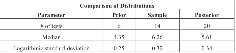
Once the prior distribution (i.e. GERS) and sample likelihood (i.e. formatted and interpreted TRS) median and standard deviations are determined, the Bayes Theorem is applied to produce a posterior distribution. The comparison of the statistical parameters of the prior distribution, sample likelihood function, and posterior distribution for the transformer of interest is presented in Table 1.
Table 1: Summary of Parameters Defining the Prior, Sample, and Posterior Distributions.
Comparison of Distributions
Parameter Prior Sample Posterior
# of tests 6 14 20
Median 4.35 6.26 5.61
Logarithmic standard deviation 0.25 0.32 0.34
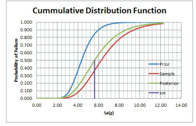
For this example, the Bayesian approach leads to a higher median in-structure capacity for the posterior distribution than if only GERS had been considered. The median of the posterior distribution is a factor of 1.29 greater than the GERS. Subsequent steps of this example show that the factor of 1.29 leads to median fragility increase of 29%. Since the Bayesian combination is comparable to a weighted average, the median of posterior distribution lies between the medians of the prior distribution and sample likelihood function, which is apparent in Figure 3.
Figure 3. Prior, Sample and Posterior Distribution CDFs
Calculation of Fragility
The Bayesian approach yielded an in-structure median capacity and associated variability in the form of a posterior distribution. The median fragility capacity, Am, can be calculated with this distribution. Say
the transformer Am was instead calculated using GERS as the capacity function and found to be 1g PGA.
To include the outcome of the Bayesian update, the new fragility was obtained by multiplying the 1g PGA by the ratios of the posterior distribution (i.e. Bayesian combination) median to the prior distribution
(i.e. GERS) median of 1.29 calculated earlier to obtain a new Am of 1.29g PGA.
In addition, the corresponding logarithmic standard deviations are necessary as inputs to an SPRA model. Assuming a CDFM (or hybrid) approach was initially followed using GERS as a capacity function to calculate a fragility and that this transformer is not located high within a structure, the EPRI (2013)
recommended betas of βc= 0.4, βr= 0.24, and βu = 0.32 were adopted.
The βr of 0.24 is entirely attributed to the randomness of the seismic input. The βu equal to 0.32 stems
from a combination of the uncertainty in the response of the structure where the transformer is located and the capacity and response of the transformer. Assuming half the βu is associated with uncertainties in
the structure and the other half with uncertainties in the transformer, the composite logarithmic standard deviation attributed to each component is 0.32/(20.5) = 0.23. Comparison of the βu of 0.23 attributed to the
uncertainty in the transformer to the βu of 0.23 for GERS per EPRI (1994) supports the assumption that
half of the variability can be assigned to each the structure and the equipment.
Because the structure remains the same in this study, the βu of 0.23 attributed to the structure was not
modified. However, the βu attributed to the equipment was updated. Again, since βr was assumed to be
entirely due to randomness in the seismic input, the βc of 0.34 determined for the posterior distribution
was taken as the updated βu of the transformers. To obtain the total βu, the SRSS of the βu of 0.23
attributed to the structure and the new βu of 0.34 attributed to the equipment yields 0.41.
Thus, the parameters to describe the updated fragility curve of the transformer based on Bayesian update of GERS are Am = 1.29g PGA, βr = 0.24 and βu = 0.41. From these values, additional parameters, HCLPF
Table 2 presents a comparison of the fragility parameters of a transformer for the case where the fragility is based solely on GERS (Case 1) and also the case where the fragility is based on the Bayesian enhancement of GERS (Case 2).
Table 2: Comparison of XFMR Fragility Based on 1) GERS and 2) Bayesian Approach.
CASE 1 2 RATIO
2/1 DESCRIPTION GERS ONLY BAYESIAN
HCLPF 0.39 0.42 1.08
βc 0.40 0.48 1.20
βr 0.24 0.24 1.00
βu 0.32 0.41 1.28
Am 1.00 1.29 1.29
Available test reports for a second equipment category were similarly studied to assess how the results of the Bayesian analysis may vary by equipment category. The results of the low-voltage switchgear (LVS) study are presented in Table 3.
Table 3: Comparison of LVS Fragility Based on 1) GERS and 2) Bayesian Approach.
CASE 1 2 RATIO OF
CASE 2/1 DESCRIPTION GERS BAYESIAN
HCLPF 0.39 0.38 0.97
βc 0.40 0.64 1.60
βr 0.24 0.24 1.00
βu 0.32 0.59 1.84
Am 1.00 1.67 1.67
SPRA SENSITIVITY STUDIES
SPRA sensitivity studies utilizing a hypothetical NPP SPRA model were conducted to assess the impact on the core damage frequency (CDF) of refining fragilities based on GERS with a Bayesian approach. Results from the Bayesian updating outlined in this paper were used in the sensitivity study. A set of four SPRA sensitivity tests were performed for transformers. Two functionally similar groups were considered in the sensitivity study, Groups A and B. The difference lies in the seismic demand on the transformers based on their locations within the plant. The sensitivity study tests are summarized as 1) all fragilities based on GERS, 2) Group A fragilities based on Bayesian approach and Group B on GERS, 3) Group A fragilities based on GERS and Group B on Bayesian approach and 4) all fragilities based on Bayesian approach. Table 4 summarizes the fragility parameters selected for sensitivity studies.
Table 4: Summary of Fragility Parameters for Components Considered in Test Cases 1-4.
GROUP A B
DESCRIPTION GERS BAYESIAN RATIO GERS BAYESIAN RATIO
HCLPF 0.54 0.62 1.15 0.53 0.60 1.15
βc 0.40 0.51 1.28 0.40 0.51 1.28
βr 0.24 0.24 1.00 0.24 0.24 1.00
βu 0.32 0.45 1.41 0.32 0.45 1.41
Case 1 was considered as the baseline. Due to unique features of the SPRA model, sensitivity tests 2 through 4 did not improve appreciably the CDF from the baseline case. This reflects that the selected transformers are not critical components in the particular SPRA model studied.
To illustrate the impact on situations where fragilities are more risk significant, we performed a second set of sensitivity studies with some hypothetical inputs. Tests 5 and 6 involved removing components that drove the model results for tests 1 through 4. Then, hypothetical fragilities were assigned to switchgear and associated transformers in the modified model which were not variable components in cases 1 through 4. The reason is that these components were identified to have higher risk significance than the transformers considered in the previous cases. Test 5, the baseline with the modified model, was performed with the switchgear and associated transformers assigned a HCLPF of 0.53g, based on GERS. Test 6, also using the revised model, was carried out with the switchgear and associated transformers assigned a HCLPF of 0.60g, based on the Bayesian analysis. Table 5 summarizes fragility parameters for components considered in test cases 5 and 6.
Table 5: Summary of Fragility Parameters for Components Considered in Test Cases 5 and 6.
GROUP Switchgear and Transformers DESCRIPTION GERS BAYESIAN RATIO
HCLPF 0.53 0.60 1.15
βc 0.40 0.51 1.28
βr 0.24 0.24 1.00
βu 0.32 0.45 1.41
Am 1.34 1.99 1.50
Sensitivity runs for tests 5 and 6 produced a CDF improvement of 2.2% from case 5 to case 6. This indicates that the use of Bayesian analysis to refine the fragilities of the switchgear and associated transformers critical to the modified model had a modest decrease to CDF.
Sensitivity runs 7 and 8 were performed to assess the impact of implementing Bayesian updating on a large scale for a SPRA model. For test case 7, all components fragilities were based on typical methods such as Experience Data, GERS, equipment-specific TRS, or analysis. The handful of components which drove the results for test cases 1 through 4 were omitted from the SPRA model similar to test cases 5 and 6. The fragilities of those components were based on conservative methods other than GERS. The rationale for omitting these components was that had their fragilities been based on more realistic methods and data, they would not have driven the results of the model. Furthermore, their fragilities are not based on GERS and consequently are not variables between the two cases. Anchorage fragility was assumed not to govern for components with functional fragilities based on GERS so that a consistent comparison can be made to the results of test case 8. Test case 8 updates all fragilities which were based on GERS in test case 7. The same ratios between the Bayesian approach and GERS only were used as in test cases 1 through 6, which are summarized in Tables 4 and 5. Sensitivity test cases 7 and 8 result in CDF improvement of approximately 6.4%. Thus, the large scale application of the Bayesian approach for the particular NPP studied shows a significant risk decrease.
decrease in CDF. Test cases 7 and 8 assessed the impact of large scale application of the Bayesian approach and a more significant decrease in CDF resulted.
CONCLUSION
A robust SPRA relies on realistic fragilities for risk significant components. The Bayesian Statistics allows for generic capacity like GERS to be updated by additional test data, providing more realistic estimates of fragilities. We assessed the impact of removable conservatism on the risk quantification. The higher median capacity coupled with higher uncertainty could impact the estimated frequency of core damage. It is recognized that relevant changes to SPRA accident sequences and risk quantification resulting from refined fragilities depend on the importance of the component(s). Refining generic fragilities of components which are risk insignificant may not have an overall effect on the SPRA results.
Within this framework, this paper addresses 1) the consistent interpretation of test data containing instances of survivals and failures, 2) a Bayesian approach to formulate a more realistic fragility with respect to GERS, and 3) the effect of removing conservatism inherent in GERS on SPRA risk quantification. More specifically, we propose a probabilistic procedure for interpreting survival and failure. The interpretation reflects that the actual failure capacity is higher than recorded when the tested specimen exhibited satisfactory performance.
This study also presents a Bayesian approach to enhance GERS for two equipment categories when additional test data are available for similar components. The updated GERS can be used to calculate a more realistic fragility for a component lacking specific seismic test reports. For the two equipment categories analyzed in this study, the proposed Bayesian approach indicates that incorporating available test data increases the median seismic fragility by a factor of 1.29 to 1.67 above that obtained solely from GERS. Plant seismic risk is clearly sensitive to conservatism inherent in estimates of functional fragilities such as GERS for critical components and insensitive for rugged or non-critical components.
REFERENCES
Benjamin, J. R. and Cornell, C. A. (1970). Probability, Statistics and Decision for Civil Engineers.
EPRI. (2009). “1019200 Seismic Fragility Applications Guide Update.”
EPRI. (2013). “1025287 Seismic Evaluation Guidance: Screening, Prioritization and Implementation
Details (SPID) for the Resolution of Fukushima Near-Term Task Force Recommendation 2.1:
Seismic.”
EPRI. (2014). “3002002933 Assessment of the Use of Experience Data to Develop Seismic Fragilities.”
EPRI. (1991a). “NP-7149-D Summary of the Seismic Adequacy of Twenty Classes of Equipment
Required for the Safe Shutdown of Nuclear Plants.”
EPRI. (1991b). “NP-5223-SL Seismic Fragility Applications Guide Update,” Revision 1.
EPRI. (1991c). “NP-6041-SL A Methodology for Assessment of Nuclear Power Plant Seismic Margin,”
Revision 1.