A Recovered Finite Volume Method for Diffusion Equations on Unstructured Grids.

(1)

Abstract

XIAO, HANPING. A Recovered Finite Volume Method for Diffusion Equations on Unstructured Grids. (Under the direction of Dr. Hong Luo).

A recovered finite volume method (RFV) for diffusion equations is presented

on unstructured grids. The RFV method is designed to provide an accurate and

robust method for computing the fluxes of the diffusion equations by removing the

interface discontinuity of derivatives of the finite volume solution. The recovered

finite volume method is implemented through: 1) In-cell recovery, in which a linear

polynomial solution in each cell is recovered from the underlying cell-average finite

volume solution. 2) Inter-cell recovery, in which the recovered linear polynomial

solution in each cell is then used to recover a continuous linear polynomial solution

on the union of two neighboring interface-sharing cells. The developed method is

analytically proved to lead to a consistent, second order five-point stencil

discretization for the diffusion equations on uniform grids, but it is proved to be

inconsistent on stretched grids. The RFV method is used to compute a variety of

problems with different tensors and non-smooth solutions on different meshes to

assess its accuracy, robustness and versatility. It has been found to be able to

provide the second order solutions on unstructured anisotropic grids and distorted

grids for smooth solutions, along with a first-order estimation for non-smooth

anisotropic problem. The resulting system of linear equations by applying the

recovered finite volume method is then solved using GMRES (generalized minimum

residual) algorithm with a variety of preconditioners. The effectiveness of different

Preconditioners and an accurate and efficient method to compute numerical

(2)

A Recovered Finite Volume Method for Diffusion Equations on Unstructured Grids

by Hanping Xiao

A thesis submitted to the Graduate Faculty of North Carolina State University

in partial fulfillment of the requirements for the degree of

Master of Science

Aerospace Engineering

Raleigh, North Carolina

2011

APPROVED BY:

_______________________________ ______________________________

Dr. Jack R. Edwards Dr. Hassan A. Hassan

________________________________

(3)

Biography

Hanping Xiao was born in Shanxi Province, China on November 06, 1986. After

graduating from TaiYuan No. 5 Middle School in 2005, Hanping earned a Bachelor of

Science in Thermal and Power Energy Engineering from Harbin Institute of

Technology, China, in 2009. From there he went to North Carolina State University,

where he is going to complete his Master of Science degree in Mechanical and

(4)

Acknowledgments

I would like to thank my advisor, Dr. Hong Luo, for his guidance and support

throughout my masters, and his considerable patience and assistance in the

completion of the current thesis work. Through him I was able to gain a great deal of

knowledge concerning CFD and advice for the future. The comments, suggestions,

and corrections from my committee members, Dr. Hassan, and Dr. Edwards are

greatly appreciated. I would also like to thank them for serving on my committee.

I also want to thank my parents and my family, who have been there for me every

step of the way through my growth, especially for the most difficult time since I

(5)

List of Figures

Figure 3.1 Calculation of gradients at cell interfaces using the divergence theorem in

2D ... 8

Figure 3.2 Calculation of gradients at cell interfaces using the modified averaging in 2D ... 10

Figure 3.3 Representation of in-cell recovery in 2D, cell i and its neighboring cells ... 12

Figure 3.4 Representation of union of cell i and cell j for inter-cell recovery in 2D ... 13

Figure 3.5 Residual equation of cell marked with “ ” only depends on its neighboring cells and neighbors of neighbors. ... 23

Figure 4.1 Grid and nomenclature for uniform Cartesian grid ... 32

Figure 4.2 Grid and nomenclature for uni-dimensionally stretched Cartesian grid... 33

Figure 4.3 Sample reconstruction, diamond path, uniform cartesian. ... 34

Figure 4.4 Gradient computation based on divergence theorem using uniform Cartesian grid. ... 35

Figure 4.5 Gradient computation based on divergence theorem using uni-dimensionally stretched Cartesian grid. ... 36

Figure 4.6 Representation of cells involved in the 13-points stencil for the recovered finite volume method.. ... 39

Figure 5.1 Computational domain Ω and meshes used in section 5.2: structured mesh (a), unstructured mesh (b), and anisotropic mesh (c). ... 46

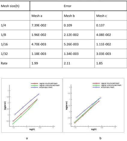
Figure 5.2 The plot of log(error) versus log(h) corresponding to Table 6(picture a) and the plot of log(error) versus log(h) corresponding to Table 7(picture b) ... 48

Figure 5.3 The Plot of Error comparison with CDG method corresponding to Table 8, test case 1 on structured mesh(Figure 5.1(a)) ... 49

Figure 5.4 Plot of log(error)_vs_log(h) corresponding to Table 9 (a) and plot of log(error)_vs_log(h) corresponding to Table 10 (b) ... 53

Figure 5.5 Solution profile for test case 3 on unstructured mesh: exact solution (a), and numerical solution (b) ... 53

Figure 5.6 Solution profile for test case 4 on unstructured mesh: exact solution (a), and numerical solution (b) ... 54

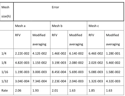
Figure 5.7 Comparisons with modified averaging method for test case 3 on structured mesh (picture a), unstructured mesh (picture b) and anisotropic mesh (picture c ) ... 55

Figure 5.8 Mesh used in section 5.2.3: Uniform triangular mesh (a), and randomly distorted triangular mesh (b). ... 56

Figure 5.9 Plot of log(error)_vs_log(h) for test case 5 (a) and Plot of log(error)_vs_log(h) for test case 6 (b). ... 58

(7)

Figure 5.11 Meshes used in section 5.2.4: symmetric uni-dimensionally stretched

mesh (picture a) and non-symmetric uni-dimensionally stretched mesh (picture b)... 60 Figure 5.12 Comparative plots of log(h)_vs_log(error)corresponding to table 13:

symmetric uni-dimensionally stretched mesh (picture a) and non-symmetric

uni-dimensionally stretched mesh (picture a) ... 62 Figure 5.13 Solution profile (a), mesh used (b), and Subdomain where solution is

negative (c) on structured mesh. ... 65 Figure 5.14 Solution profile (a), mesh used (b), and Subdomain where solution is

negative (c) on unstructured mesh ... 66 Figure 5.15 Solution profile(a), mesh used(b), and Subdomain where solution is

negative(c) on and anisotropic mesh ... 67 Figure 5.16 Solution profile(a), mesh used(b), and Subdomain where solution is

negative(c) on structured mesh with a hole at the center ... 68 Figure 5.17 Solution profile for test case 10 on computational domain with a square

hole (shown in Figure 5.16(b)) ... 70

Figure 5.18 Chess board distribution of the parameters of tensor D3 and minimum

values of each subdomain, with fixed k₁1000, k₂ 1 ... 72 Figure 5.19 Profile of discrete solution corresponding to Figure 5.18 (a) and

subdomain where solution is negative (b) ... 73

Figure 5.20 Chess board distribution of the parameters of tensor D3 and minimum

values of each subdomain, with changing k1 and k2 ... 73

Figure 5.21 Profile of discrete solution corresponding to Figure 5.20 (a) and

subdomain where solution is negative (b) ... 74 Figure 5.22 Mesh before being distorted (picture a); randomly distorted mesh with

k=0.4 (picture b); randomly distorted mesh with k=0.8 (picture c) used in section 5.6 ... 76 Figure 5.23 Plot of Log(error) vs log(h) for test case 12 corresponding to Table 16 ... 77 Figure 5.24 Convergence history versus time steps (a) for test case 13 on structured

mesh using different schemes: Explicit, GMRES, GMRES+Diagonal, GMRES+LU-SGS, GMRES+ILU. And Convergence history versus CPU time (b) for test case 13 on structured mesh using different schemes: Explicit, GMRES, GMRES+Diagonal,

GMRES+LU-SGS, GMRES+ILU ... 81 Figure 5.25 Convergence history versus time steps (a) for test case 13 on

unstructured mesh using different schemes: Explicit, GMRES, GMRES+Diagonal, GMRES+LU-SGS, GMRES+ILU. And Convergence history versus CPU time (b) for test case 13 on unstructured mesh using different schemes: Explicit, GMRES,

GMRES+Diagonal, GMRES+LU-SGS, GMRES+ILU ... 82 Figure 5.26 Convergence history versus time steps (a) for test case 13 on anisotropic

(8)

GMRES+ILU. And Convergence history versus CPU time (b) for test case 13 on anisotropic mesh using different schemes: Explicit, GMRES, GMRES+Diagonal,

GMRES+LU-SGS, GMRES+ILU ... 83

Figure A1. Representation of in-cell recovery in 1D, cell i and its neighboring cells... 90

Figure A2. Representation of union of cell i and cell i+1 for inter-cell recovery in 1D... 91

(9)

List of Tables

Table 1. Effectiveness of numerical Jacobian evaluation using CPR scheme ... 26

Table 2. Maximum condition number on the structured meshes(shown in Figure5.1(a)) ... 43

Table 3. Maximum condition number on the unstructured meshes(shown in Figure5.1(b)) ... 43

Table 4. Maximum condition number on the anisotropic meshes(shown in Figure5.1(c)) ... 44

Table 5. Maximum condition number using QR approach and normal equation approach on different kinds of meshes. ... 44

Table 6. Analysis of accuracy for test case 1 on different meshes ... 47

Table 8. Error comparison with CDG, test case 1 on structured mesh [9] ... 49

Table 11. Analysis of accuracy for test case 5 and test case 6 on randomly distorted triangular meshes ... 58

Table 12. Error comparison with non-linear FV method, test case 6 on distorted meshes [2] ... 59

Table 13. Analysis of accuracy for test case 7 on symmetric uni-dimensionally stretched mesh and non-symmetric uni-dimensionally stretched mesh ... 61

Table 14. Computed Maximum and minimum values on different meshes used in section 5.3 ... 65

Table 15. Analysis of accuracy for test case 10 on computational domain with a square hole (shown in Figure 5.16(b)) ... 70

Table 16. Analysis of accuracy for test case 11... 77

Table 17. Condition number for different distortion parameters using test case 12 ... 78

Table 18. Time steps and CPU time needed for a variety of preconditioners on structured mesh (shown in Figure5.1(a)) ... 80

Table 19. Time steps and CPU time needed for a variety of preconditioners on unstructured mesh (shown in Figure5.1(b)) ... 81

(10)

1 Background Introduction

In recent years, a great deal of effort has been made in developing finite

volume methods to solve the compressible Navier-Stokes equations on unstructured

grids. There exist two major classes of the finite volume methods: cell-centered and

vertex-centered finite volume methods. A vertex-centered finite volume method is

more popular when used for discretizing the viscous fluxes in the Navier-Stokes

equations, since it avoids the difficulty for the discretization of the viscous fluxes by

using a hybrid formulation, where the discretization of the inviscid fluxes is carried

out via vertex-centered finite volume and finite element approximation is used for

the discretization of the viscous fluxes. The cell-centered finite volume method is

also widely used to solve compressible Navier-Stokes equations in engineering due to

the satisfaction of the integral form of the conservation law and its simplicity of

implementation. However, it does not possess the natural tools for gradient

calculation and interpolation [7]. In the case of structured grids, the discretization of

the diffusive fluxes is straightforward, where the gradients are usually estimated by

central differencing in the corresponding curvilinear coordinates direction.

However, the approximation of gradients using a cell-centered finite volume method

is considerably more complicated on unstructured grids.

Any ideal scheme for discretization of viscous fluxes should have the following

(11)

I have higher than the first order of accuracy for smooth solutions;

II be locally conservative;

III be monotone, i.e. preserve positivity of the differential solution;

IV be reliable on unstructured anisotropic meshes that may be severely distorted;

V allow heterogeneous full diffusion tensors;

VI be compact.

Researchers have suggested a lot of methods for gradient

reconstruction/recovery based on finite volume methods. Some linear schemes [3, 4,

5, 8, 33, 34, 35] have been developed to evaluate the gradients of the flow variables

at the interfaces. Though all of them have one or more of above desired properties,

no linear scheme possessing all of the six properties has been developed. There are

two common approaches suitable for unstructured grids, which are frequently used

in the literature to estimate the gradients of the flow variables at the cell interfaces:

1) Gradient computation based on divergence theorem [8], i.e. so-called diamond

control volume. 2) Gradient computation based on a modified averaging of gradients

[33, 34, 35]. Unfortunately, neither of these two methods can achieve accuracy and

positivity simultaneously on arbitrary grids according to the detailed analysis by

Coirer [37] and Haselbacher [36]. Moreover, both of them are not compact and not

consistent on highly distorted grids.

Discontinuous Galerkin methods (DG) have also been used for solving diffusion

(12)

discontinuous galerkin) methods for convection-diffusion problems. This method is

attractive due to its extremely high parallelizability and its high-order accuracy. More

recently, J. peraire [9] presented a compact discontinuous Galerkin (CDG) method

for an elliptic model. CDG method is related to the LDG method, but unlike the LDG

method, the sparsity pattern of the CDG method only involves nearest neighbors and

the CDG method works without stabilization for an arbitrary orientation of the

element interfaces [9]. These two methods are working well without a

heterogeneous full diffusion tensor. However, no numerical experiment has been

performed to test heterogeneous full diffusion tensors or to prove the monotonicity

in [9, 10].

It is clear that the most difficult requirement to be satisfied is the monotonicity,

which guarantees the solution of a system of linear algebraic equations will be

non-negative for any non-negative right-hand side [15]. Ordinary finite element

method and finite volume method fail to preserve monotonicity for full diffusion

tensors or on general meshes [6, 15]. Some non-linear schemes satisfying the

monotonicity on unstructured meshes have been proposed by Burman and Potier

[13,14]. However the numerical experiments in [14] showed that the scheme is

monotone only when solving parabolic equations with sufficiently small time steps.

Lipnikov [2] further developed and analyzed the non-linear finite volume scheme

proposed in [14] by giving correct positions of collocation points for the case of a full

(13)

improve robustness of the scheme for problems with strong anisotropy and sharp

gradients.

Although non-linear schemesthat have all six properties for solving diffusion

equations are available, the extension of these non-linear schemes for discretizing

the viscous fluxes in the Navier-Stokes equations is not straightforward. The main

objective of effort discussed in this work is to derive a recovery scheme possessing as

many properties as possible based on cell-centered finite volume method for

diffusion equations and this scheme can be directly extended for discretizing the

viscous and heat fluxes in the compressible Navier-Stokes equations. First, starting

from the cell-average finite volume solution, a piecewise linear polynomial solution

on the union of two cells adjacent to an interface is recovered by the processes of

in-cell recovery and inter-cell recovery. Second, methods for solving the

over-determined systems generated by inter-cell recovery are discussed. Third, we

analytically demonstrate the present scheme is second order of accuracy using one

dimensional uniform grid. Fourth, the RFV scheme is numerically proved to preserve

second order of accuracy imposing no constraints on analtical functions, tensors.

Fifth, monotonicity (in the sense of solution positivity) of this scheme is tested under

a variety of conditions. Sixth, numerical experiments are performed to solve

non-smooth anisotropic problem and to compute problems with heterogeneous

(14)

parameters are studied to investigate the ability of this scheme to deal with seriously

distorted meshes.

Another objective of this work is to compare the effectiveness of techniques

for solving systems of linear equations. Applying the present RFV method rises a

system of linear equations (ncellncell ), which can be solved explicitly to achieve a

steady-state solution using a pseudo-time approach. Although, explicit methods

require only limited storage and are easy to implement, the rate of convergence of

explicit methods slows down dramatically for large-scale problems, resulting in

inefficient solution techniques [17]. In order to improve convergence, implicit

methods such as iterative solution methods and approximate factorization methods

are developed [see, e.g.18, 19, 20]. One of the most successful iterative methods is

GMRES algorithm using the Krylov subspace method [21]. GMRES algorithm with

Preconditioners has been widely used for solving non-symmetric linear systems due

to its high efficiency. The effectiveness of preconditioners such as diagonal

preconditioner, Lower-Upper Symmetric Gauss Seidel (LU-SGS) preconditioner and

Incomplete Lower Upper (ILU) preconditioner are compared and an accurate and

efficient method to compute numerical Jacobian matrix is also discussed in this work.

The outline of the paper is structured as follows: The diffusion problem is formulated

in chapter 2. Numerical method is presented in chapter 3. An assessment of

numerical methods is analyzed in chapter 4. Numerical experiments are reported in

(15)

2. Problem Definition

Let Ω be a two-dimensional bounded computational domain with boundaries

N

D 

   

  . _Ddenotes the boundaries with Dirichlet boundary condition,

and N the boundaries with Neumann boundary condition. The diffusion

problem is defined as:

(Du) f in 

D

g

u on _D_(2.1)

N

g n u

D 

 

on N

where f is a given function and u=u(x,y) is analytical function to be determined. n

(16)

3. Numerical Method

Finite volume methods are employed to solve diffusion equation by integrating

diffusion equation (2.1) over cell i, to give:

(DU) (3.1)

where i is the volume of cell i in the context of finite volume method in

three-dimensional space (3D), and is the area of cell i in two-dimensional space (2D).

Then applying green’s theory to equation (3.1), equation (3.2) is obtained as:

(DU|_f)n (3.2)

where j

y U i x U U

f f

f

 



     

 | , i.e. the gradients at faces of , and

f

x U  

,

f

y U  

are the components of gradients in x and y directions respectively.

Since F is a known function, the integration of F, i.e., the right hand side of

equation (3.2) can be trivially obtained. Now the objective is to recover or

reconstruct continuous gradients at faces U _f, using underlying cell-average finite

volume solution.

3.1 Common Approaches Used in the Literature

Two common approaches frequently used in the literature to estimate the

gradients of the flow variables at the cell interfaces are presented in this section: 1)

Gradient computation based on divergence theorem. 2) Gradient computation based

(17)

highly depend on meshes. A compromise between accuracy and positivity has to be

made since they cannot be achieved simultaneously on arbitrary meshes [36, 37].

Approach 1: Gradient computation based on divergence theorem

Coirer [37] developed a method for the computation of the gradients at cell

interfaces using the divergence theorem. A so-called diamond control volume is

formed by connecting the two vertices of a face with the centroids of cells which

share the interface, see Figure 3.1(a). The values of variables at the vertices are

determined by weighted-averaging based on the pseudo-Laplacian formula [38], see

Figure 3.1(b).

(a) Diamond control volume (b) Averaging at a node

Symbol legend: cell centroid, node, target interface,

faces of diamond control volume

(18)

This approach is obviously not compact, and even not grid-transparent, since

information from node-sharing cells is needed to estimate the averaged values at the

vertices as shown in Figure3.1(b).

Approach 2: Gradient computation based on modified averaging

A different approach for the computation of the gradients at the cell interfaces

is based on modified averaging of gradients. An initial value for the gradient at the

cell interfaces may be obtained by simply averaging the gradients of the two adjacent

cells, UL



(left cell), and UR



(right cell), to give

) (

2 1

R L

avg U U

U   

   (3.3)

This scheme leads to an odd-even point decoupling, that can be remedied by

applying a correction in the direction

L R

L R RL

r r

s _ _

  

 

 , where r_R and r_L denote

position vectors for the center of the left and right cells. sRL 

is the unit vector that

connects the centroids of the left cell and the right cell of the interface. The gradient

of the interface is finally obtained as:

RL L R

L R RL avg avg

face _r _r s

U U s U U

U      



) (

       

 (3.4)

Although approach 2 is not compact, since it involves the neighbors of the

neighbors due to the computation of gradients in each cell, it is grid-transparent, see

(19)

Symbol legend: cell centroid, node, target interface

Figure 3.2Calculation of gradients at cell interfaces using the modified averaging in 2D.

Unfortunately, neither of these two approaches possesses all the properties

given in the background introduction of this paper. Both of them are not consistent

on non-uniform meshes, and neither of them can satisfy discrete maximum principle

(DMP) without imposing severe restrictions on both meshes and problem

coefficients, as shown in chapter 4. A detailed accuracy and consistency analysis of

these methods is presented in chapter 4. Indeed, a second order cell-centered

grid-transparent finite volume scheme on non-uniform and highly distorted grids for

diffusion equations is still at large.

3.2 Recovered Finite Volume Scheme

(20)

presented for solving the diffusion equation on triangular grids. The developed RFV

can be extended for the discretization of the viscous and heat fluxes in the

Navier-Stokes equations. The RFV method is established by the following two steps:

In-cell recovery and Inter-cell recovery.

First step: In-cell recovery

In-cell recovery recovers a piecewise linear polynomial solution in each cell

from the underlying cell-average finite volume solution. The linear polynomial

solution in cell i can be expressed as:

i i i

i i

i

y U y y x U x x U U

       

 ( ) ( ) (3.5)

where and are gradient components of cell in x and y directions

respectively, and Ui is cell-average value of .

We consider cell and its three face-neighboring cells: , ,and ,

shown in Figure 3.3. Imposing that the integral of ui is equal to the integral of each

of its neighboring cells respectively yields:

(3.6)

Equation (3.6) leads to three equations as following:

(21)

Figure 3.3Representation of in-cell recovery in 2D, cell i and its neighboring cells.

Since the dimension of the polynomial space is three, we have three basis

functions:

1

1

B , B2 xxi, B3 yyi (3.8)

The basis functions should be normalized to improve the conditioning as:

1

1 

B , B₂ (xx_i)/x, B₃ (yy_i)/y (3.9) where x0.5(max(x)min(x)) , and y0.5(max(y)min(y)) , and max(x),

max(y) are the maximum coordinates in the cell , while min(x), min(y) the

minimum coordinates. Equation (3.7) can then be rewritten in matrix form as:

(22)

Solving the over determined system (3.10) based on the least-squares sense,

the two unknowns , and are obtained.

Second step: inter-cell recovery

Inter-cell recovery estimates a piecewise linear polynomial solution on each

union (as shown in Figure 3.4) composed of two adjacent cells based on recovered

linear polynomial solution in each cell by using a Taylor series expansion at the

centroid of the union. The linear solution of the union can be expressed as:

ij ij ij

ij c

R ij

y U y y x U x x U U

       

 ( ) ( ) (3.11)

where Uc represents the value of variable at the centroid of union of i and j,

ij

x and yij the coordinates of the centroid, and ij

x U  

,

ij

y U  

gradients of solution

U in the union of i and j.

Figure 3.4Representation of union of cell i and cell j for inter-cell recovery in 2D

Equation (3.11) can be further expressed using cell-average value:

j

(23)

ij ij ij ij ij R ij y U y y x U x x U U        

 ( ) ( ) (3.12)

where Uij is the cell-average value in the union.

Inter-cell recovery is accomplished by requiring:

           



    j k j j k R ij i k i i k R ij d B u d B u d B u d B u j j i

i _{k=1,2,3 (3.13)}

where B₁_i 1 , B2i xxi , B3i  yyi for i and B1j 1 , B2j xxj ,

j

j y y

B3   for j， B1ij 1 , B2ij  xxij, B3ij  yyijfor the union of i and

j

 ，and Ui , Uj are piecewise linear polynomial solution:

,

. （3.14）

Equation (3.13) yields 6 equations, and there are three degrees of freedom, i.e.

three unknowns (U_ij ,

ij x U   , ij y U  

) are to be determined, so this is an

over-determined system(63). Note that the RFV scheme has to obey the conservation. In this case, the cell-average value Uij can be obtained by

conservation: j i j j i i ij U U U      

 (3.15)

Michael Dumbser [22] solved over-determined systems like this using the

constrained least-squares technique by introducing Lagrange Multiplicator  .

(24)

(), thus equations (3.13) become a system of 6 equations and 4 unknowns. On the

contrary, we are trying to reduce one degree of freedom by taking Uij as a constant,

since to calculate Uij is trivial (the constrained least-squares technique also

requires the computation of U_ij).

Actually, when B1 1, Equation (3.11) leads to the following two equations:

                                            



    j j j j j j j i j ij ij ij ij ij i i i i i i i ij ij ij ij ij d y U y y x U x x U d y U y y x U x x U d y U y y x U x x U d y U y y x U x x U i i ) ) ( ) ( ( ) ) ( ) ( ( ) ) ( ) ( ( ) ) ( ) ( ( (3.16)

Simply solving these two equations in (3.16), we also get

j i j j i i ij U U U        .

In this sense, if we take Uij as a constant, two of the six equations in (3.13) have

already been used to compute Uij. However, the solution from the remaining four

equations and 2 unknowns are different from the solutions obtained using the

constrained least-squares technique. In the present work, we involve the first two

equations (3.16) again and then the linear system becomes a (62) system, instead of (64) with constrained least-squares technique. This simplified system

of 6 equations and 2 unknowns leads to the same solution as the constrained

least-squares technique.

Again, the basis functions should be normalized to improve the conditioning:

1

1i 

B , B2i (xxi)/xi , B3i (yyi)/yi for i

 _and ₁

1j 

B ,

j j

j x x x

(25)

ij ij

ij y y y

B₃ (  )/ for the union of i and j.

where xi, yi, xj, yj, xij , yij are half of the maximum coordinates

minus the minimum coordinates in the cells , , , respectively, i.e.

)) min( ) (max( 5 .

0 x x

x 

 , and y0.5(max(y)min(y))_.

Equation (3.13) can then be rewritten in matrix form as:

                                                                                                                                              



                        j j i i j j i i i i i j i j j i j i j i i i j j j j j j j j j j i i i i i i i i i i j j j j j j j j j j i i i i i i i i i i j j ij j j i ij i i ij ij ij j j ij i i ij j j ij j j ij i i ij j j ij i i ij j ij i ij i i ij j j ij i ij d B B y y U d B B x x U d B B y y U d B B x x U d B B y y U d B B x x U d B B y y U d B x x U d U d U d U d U y y U x x U d B B d B B d B B d B B d B B d B B d B B d B d B d B B d B d B 3 3 3 2 3 3 3 2 2 3 2 2 2 3 2 2 ij 3 3 3 3 2 3 3 2 3 2 2 2 2 3 3 3 2 2 2 2 B

（3.17）

Note that some coefficients of (3.17) are of the form of integral of quadratic

function. This over-determined linear system of 6 equations for 2 unknowns can be

solved in the least-squares sense by normal equation approach or QR decomposition

approach. The conditioning of these two methods will be discussed in chapter 4.

Order of accuracy of the developed RFV scheme is analytically proved using

non-uniform mesh in one space dimension for the sake of brevity, see appendix A.

3.3 Boundary Conditions

Both of Dirichlet boundaries (D) and Neumann boundaries (N) can be

(26)

Dirichlet boundary condition:

Dirichlet boundary condition specifies the solution values on the boundary of

the domain. The values of ghost cells, which are required in the process of in-cell

recovery, are set as:

i b

g U U

U 2  (3.18) where Ugdenotes the value of the ghost cell, Ub the value of boundary and Ui

the value of boundary cell adjacent to the ghost cell.

The gradients of boundary faces are obtained by the process of inter-cell

recovery. The union, in which a linear polynomial is recovered, includes a boundary

cell and a ghost cell, but the gradient of the boundary is computed using only three

equations from boundary cell by one-side inter-cell recovery as:

i k i i k R

ijB d u B d

u

i i

 



_



 

, k=1,2,3 (3.19)

Neumann boundary condition:

Neumann boundary condition specifies the values the derivative of a solution is to take on the boundary of the domain. The values of ghost cells that are also

needed for Neumann boundary condition in in-cell recovery are estimated by:

) (

)

( _g _i

f i

g f i

g y y

y U x

x x U U

U 

    

 

 (3.20)

where Ugdenotes the value of the ghost cell, Ui the value of boundary cell

(27)

centroid of ghost cell, and

f

x U  

,

f

x U  

the gradients of boundary faces. Note that

the gradients of boundary faces are given. Therefore there is no need to compute

gradients of boundary faces where Neumann boundaries are imposed.

3.4 Solvers of Linear Systems

3.4.1 Explicit Method

The simplest method to obtain a steady-state solution is to solve equation (3.4)

explicitly by introducing a pseudo time term:

i f

i D U nds Fd

d t U

i i

i

 

  

  



 

 

 

) (

(3.21)

Using R_i(x) to denote D U _f nds Fd i

i i

 







 



 

)

( , which has been calculated by

the process of recovery, and replacing d i

t U

i

  





with i

n i n i

t U U

 

 1

, equation (3.21)

becomes:

) ( R_i 1

x t U U

i n i n

i _

  



(3.22)

) (

R_i x is the right-hand-side residual that is equal to 0 for steady state. It is easy to update solutions explicitly according to equation (3.22). However, low

convergence rate of explicit methods results in hundreds of thousands of time steps

to achieve a steady state for large scale problems. Therefore, it is desirable to employ

(28)

3.4.2 GMRES (generalized minimum residual) Method

GMRES algorithm combined with a variety of preconditioners is used to solve

the systems of equations in this work. GMRES approximates the exact solution of

b u

A (3.23)

by minimizing the norm of the residual Au-b. The use of preconditioners is to

reduce the condition number of a problem, so that the given problem is more

efficient and robust for GMRES. The preconditioned GMRES involves solving an

equivalent linear system:

b ~ u A~

 _

(3.24)

by pre-multiplying the original linear system with some preconditioning matrix P:

b P u A

P-1  1

(3.25)

The best preconditioning matrix for A would cluster as many eigenvalues as

possible at unity, therefore, the optimal choice of P is A, in which case the underlying

matrix problem for GMRES is trivially solved with one Krylov vector [17]. In the

present work, three preconditioners: diagonal preconditioner( PD), LU-SGS

preconditioner(P(DL)D-1(DU)), and ILU preconditioner(PL~U~) are used to test their effectiveness.

L, D, and U are strictly lower part, diagonal, and upper part of numerical

(29)

3.4.3 Numerical Jacobian Matrix

The Jacobian matrix can be defined as:

                                       n n n n n n x R x R x R x R x R x R x R x R x R     2 1 2 2 2 1 2 1 2 1 1 1 R x

J（） (3.26)

However, The analytical Jacobian becomes more and more difficult as the

complexity of discretized residual equations increases, which makes it impossible to

always use analytical Jacobian. Numerical Jacobian evaluation has been used to

approximate the analytical Jacobian calculation by adding a small number  as

perturbation in the finite difference method. The numerical Jacobian can be

estimated by one-sided derivatives as [24]:



 ) ( )

(x e R x

R

x

R i j i

j i           (3.27) where              0 1 0   j

e is the th

j unit vector, in which the value of the th

j component

is one, while the values of all other components are zero.

Typically, two disadvantages occur when it comes to Numerical Jacobian. One

is the accuracy problem and the other is that to obtain the numerical Jacobian may

cost long computation time.

(30)

perturbation magnitude  , since  is related to both truncation error and

condition error [25]. While truncation error is associated with neglected terms in the

Taylor’s series expansion, condition error is due to loss of computer precision. Sang

and Jae [24] developed a method to find a perturbation magnitude with minimum

error. According to this method, the total error in the numerical calculation of the

first derivative of function f(x) is expressed as:

2 ) ( 2

)

( ₂

2  

 

x f E

E R

total _

 

 (3.28)

where E_R is round-off error due to the machine precision.

The first term of equation (3.28) comes from condition error and the second

term is caused by truncation error. It is observed from equation (3.28) that if  is

relatively large, truncation error is the main error and if the  is relatively small, condition error becomes the dominant factor. The optimal perturbation magnitude

 is the one that makes Etotal the smallest by differentiating Etotal with respect

to :

0 ) ( 2 1 2 ) (

2 2

2  

     

x f E

E_total _R 

 



(3.29)

Assuming the order of the second derivative to be one may not introduce large

errors, and the bound of round-off error is the precision error which can be taken as

the machine zero for both single and double precision cases[24]. Equation (3.29)

becomes:

M opt2 E

(31)

where E_M is machine zero that depends on both computers and compilers.

All the calculations of this study are realized on a 2.67 GHz Inter Xeon W3520

CPU with gfortran compiler using double precision. Machine zero is defined as the

smallest number that the computer can recognize. In this work, E_M is estimated as

follows:

    

 

 

2 Repeat )

0 . 1 0

. 1 (

2 2

1 1

M

M M

M

E if

E E

E

(3.31)

Numerical experiments according to equation (3.31) show that E_M of the

machine we use is 16

10 22 .

2   . Machine zero can also be obtained by using internal function of ifort compiler: E_M epsilon(x). If x is declared to be a single precision variable, the output will be the machine zero of single precision while if x is declared

to be a double precision variable, the output will be the machine zero of double

precision.

The numerical Jacobian matrix is composed of partial derivatives of each

residual R(x) with respect to every variable. The main computation work is due to the

need for calculating the residual vector with each perturbed variables for all cells.

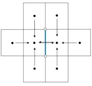
Fortunately, most of the derivatives are zero since the residual equation only

depends on the given cell itself, its face-sharing neighbors and neighbors of

neighbors (Figure3.5). On 2D triangular meshes, residual equation of a particular cell

(32)

neighbors of nearest neighbors, so perturbed residual equations are computed only

with variables in these cells to reduce the computation time.

Figure 3.5Residual equation of cell marked with “ ” only depends on its neighboring cells and neighbors of neighbors.

A direct method to implement this idea is to calculate one single residual

equation Ri rather than the whole vector R 

using a subroutine. But, this would

require calling the subroutine for thousands of times, and a large number of

calculations for gradients recovery which can be reused are recalculated in the

process of computing residual equations separately. A more efficient method

proposed by Curtis, Powell and Reid (CPR scheme) has been used to reduce the

computation time in the present work. CPR scheme divides the columns of Jacobian

matrix into groups in such a way that the first group is established by including each

column that has no non-zero entry in the same row and the other groups are formed

(33)

in any group[32]. The initial residual vector R(x) is obtained by using initial value of

x(subroutine call is needed once), and one further subroutine call is needed for each

group by changing all variables x which correspond to the columns included in a

given group by  . Suppose that the columns of Jacobian matrix can be divided into

m groups, then the total number of subroutine calls required is reduced from n+1 to

m+1, where n is the number of cells or the number of columns. Note that although

we can apply CPR scheme to any matrix, the improvement for non-sparse matrices is

little, if any. For example, applying CPR to a full matrix may lead to n groups which

means each column itself becomes a group. In this special case, CPR scheme cannot

reduce computation time. The best CPR can do is to compact all columns of a matrix

into only one group, which happens when CPR scheme is applied to any diagonal

matrix.

Example:

By applying CPR scheme to a tri-diagonal matrix as below, column1 and 4 are

included in group1; column2 and 5 are included in group2; column3 and 6 are

included in group3, and thus this tri-diagonal matrix is divided into 3 groups and 3

subroutine calls are needed to evaluate the whole Jacobian matrix.

G1: C1+C4 G2: C2+C5 G3: C3+C6 Applying CPR 6 5 4 3 2

1 C C C C C

C                   66 65 56 55 54 45 44 43 34 33 32 23 22 21 12 11 0 0 0 0 0 0 0 0 0 0 0 0 0 0 0 0 0 0 0 0 B B B B B B B B B B B B B B B B 3 2

1 G G

(34)

Note that when we only need the diagonal entries of the Jacobian matrix (for

example if diagonal preconditioner is used), the number of groups can be even less,

since we just need to make sure that no non-zero entries are included in the same

row position where a diagonal element exists. The same tri-diagonal matrix can be

divided into only two groups and only 2 subroutine calls are needed to evaluate all

diagonal entries of Jacobian matrix.

G1: C1+C3+C5

G2: C2+C4+C6 Applying CPR

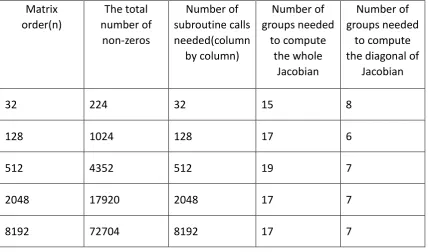
For all numerical experiments used in this work, the number of groups needed

is between 15 and 19 by applying CPR scheme to the Jacobian matrices. For example,

the Jacobian matrix of a 64cells64cells mesh, which has 8192 columns, can be divided into 17 groups, so that the subroutine calls are reduced from 1+8192 to 1+17

for the whole Jacobian matrix. The same matrix is compacted into only 7 groups for

evaluation of diagonal entries of Jacobian matrix, see Table. 1.

6 5 4 3 2

1 C C C C C

(35)

Table 1

Effectiveness of numerical Jacobian evaluation using CPR scheme.

Matrix order(n)

The total number of

non-zeros

Number of subroutine calls needed(column

by column)

Number of groups needed

to compute the whole

Jacobian

Number of groups needed

to compute the diagonal of

Jacobian

32 224 32 15 8

128 1024 128 17 6

512 4352 512 19 7

2048 17920 2048 17 7

(36)

4 An Accuracy and Positivity Analysis of Numerical Methods

for Diffusion Equation

Two existing common methods and the developed RFV method for diffusion

equations have been presented in chapter 3. A detailed accuracy and positivity

analysis of these methods is studied in this chapter.

4.1 Tools Needed to Assess the Accuracy and Positivity

Laplace’s equation:

It is convenient to assess the discretization of diffusion equation or the viscous

terms of Navier-Stokes equations by investigating the discretization of Laplace’s

equation since the viscous term is reduced to Laplace’s operator, for incompressible

flows and constant viscosity. Laplace’s equation is written as:

0

2 

 U (4.1)

Equation (4.1) can also be obtained from diffusion equation (2.1) by setting

diffusion tensor D to be constant and right hand side f to be 0.

Discrete maximum principle (DMP):

Maximum principle that is held by the solution of Laplace’s equation, states that the maxima of a function appear on the boundaries of the domain. When

Maximum principle is interpreted on a discrete level, the DMP implies that the value

(37)

conditions upon the coefficients in the stencil so that the approximation can satisfy

the DMP. If a stencil obtained by some method to solve Laplace’s equation is an

N-points stencil, it can be written as:

0 )

(

0

2   







N

i i iU

U L

U 



(4.2)

where N denotes the total number of the support cells, and i the coefficients in

the stencil. The support cells used contain at least the nearest neighbors to U0. Thus

equation (4.2) can be rewritten for solving U0 as :





 N

i i iU

U

1

0  (4.3)

where

0

 

 i

i  . The discrete maximum principle then requires that U0 is

bounded by its neighboring cells:

) , , max( )

, ,

min(U₁ U₁ U_N U₀  U₁U₁ U_N (4.4) A sufficient condition to satisfy (4.4) is to require all the coefficients of its

neighbors to be non-negative, i.e. i 0. A scheme satisfying (4.4) discretely

preserves an important physical property of the Laplacian: it satisfies the maximum

principle.

Accuracy:

The accuracy of the discretization of diffusion equation is investigated by

(38)

2 2 0 2 2 2 0 2 0 0 0 ) ( 2 1 ) ( 2 1 ) ( ) ( ) ( y U x U y U x U U L N i i i N i i i N i i i N i i i N i i             



                  



 x y

U N i i i i 2 0 ) ( 2

1 ___

(4.5)

where i  xi x0, i  yi y0.

For a discretized Laplacian to have a truncation error of second order, the

following set of conditions for the i must be met:



  N i i 0 0

 (4.6)



  N i i i 0 0 

 (4.7)



  N i i i 0 0 

 (4.8)



  N i i i 0 2 2 

 (4.9)



  N i i i i 0 0  

 (4.10)



  N i i i 0 2 2 

 (4.11)



  N i i i 0 3 0 

 (4.12)



  N i i i i 0 2 0  

 (4.13)



  N i i i i 0 2 0  

(39)





N

i i i 0

3 0



 (4.15)

The conditions given by equation (4.6) to (4.15) guarantee a consistent, second-order

approximation, while the conditions set by equation (4.6) to (4.11) lead to a

consistent first-order approximation. The Laplace operator can then be written as :

) ( )

(U 2U O h2

L   (4.16)

for a second-order accurate method, and a first-order accurate scheme can be

written as:

) ( )

(U 2U O h

L   (4.17)

where h is the mesh size.

Consistency:

The Laplacian that is found to be :

) ( ) (

1 ) (

)

( ₂

2 5 2 4 2 2 3 2

1 O h

y U k y x

U k x

U k h y U k x U k U

L 

              

 (4.18)

is termed consistent if all of the following requirements (given by equation (4.19 to

4.23)) are satisfied:

0

1 

k (4.19)

0

2 

k (4.20)

1 3 

k (4.21)

0

4 

k (4.22)

1 5 

k (4.23)

(40)

inconsistent, and if either k₁ 0 and/or k₂ 0, this type of truncation error will be termed as dangerously inconsistent. In this case, the error increases when the

mesh is refined and even grid convergence to the wrong solution can never be

achieved. Both of inconsistent and dangerously inconsistent approximations should

be avoided.

4.2 An Assessment of Numerical Methods for Diffusion Equation

An assessment of some common schemes used in the literature to estimate

the gradients at the cell interfaces is made in this section. The accuracy is analyzed

by applying Taylor series expansion to Laplace equation on the following two types of

grids: uniform Cartesian grid and uni-dimensionally stretched Cartesian grid, as

shown in Figure 4.1 and Figure 4.2. The assessment of positivity is then obtained by

examining the coefficients of the stencil.

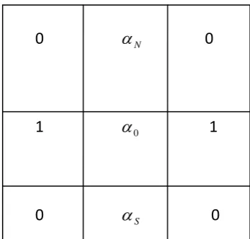
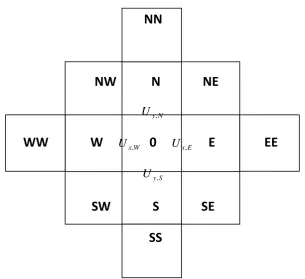
4.2.1 Model Grid Topologies and Formulae

The Laplace operator on the model grid topologies is shown in this section.

The Laplace operator on the uniform Cartesian grid (shown in Figure 4.1) for U0 is

given by:

) (

1 )

( ₀ U_x_,_E U_x_,_W U_y_,_N U_y_,_S h

U

L     (4.23)

where Ux,E, Ux,W, Uy,N, and Uy,S denote the recovered/reconstructed gradients

(41)

NW N NE h

N y

U ,

W Ux,W 0 Ux,E E h

S y

U _,

SW S SE h h h h

Figure 4.1Grid and nomenclature for uniform Cartesian grid.

For the uni-dimensionally stretched Cartesian grid (shown in Figure 4.2), the

Laplace operator for U0 reduces to :

)] (

[ 1 )

( ₀ U_x_,_E U_x_,_W U_y_,_N U_y_,_S h

U

L     (4.24)

The cells of the uni-dimensionally stretched Cartesian grid are only stretched in the

y-direction uniformly. The stretching ratio  is defined as:

S N

y y y

y

    

 0

0

 (4.25)

and the aspect ratio is given by:

0

y h

 

 (4.26)

so that the distances in centroid heights is :

  



2 ) 1 (

0 0

  

h y y

S N

(42)

where yN, y0 and yS are the centroid of North, 0 and South cells in y-direction.

NW N NE yN

W 0 E y0

SW S SE yS

h h h

Figure 4.2Grid and nomenclature for uni-dimensionally stretched Cartesian grid.

4.2.2 An Accuracy and Positivity Analysis

An assessment is made to analyze the numerical methods for diffusion

equation introduced in chapter 3. The accuracy and positivity of these methods are

examined using grids of different types as shown in section 4.2.1.

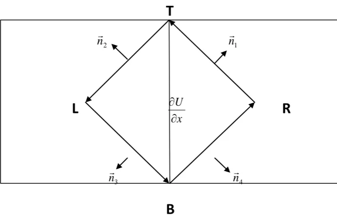
Gradient computation based on divergence theorem:

This method reconstructs the gradients at each face by applying the

divergence theorem to a diamond control volume formed by connecting the two

vertices of a face with the centroids of cells which share the interface as described in

Figure 3.1(a). According to divergence theorem, the integral around the diamond

(43)

T

n₂ n₁

L

x U  

R

n3 

n₄

B

Figure 4.3Sample reconstruction, diamond path, uniform cartesian

Thus the reconstructed gradient

x U  

is computed as:

) 2

2 2

2 (

1 1, 2, 2, 3, 3, 4, 4, 1, R x x B x x L x x T x x

U n n U n n U n n U n n x

U 

 

   

(4.28)

where  is the area of the co-volume. n1,x, n2,x, n3,x and n4,x denote the

x-components of n1 

, n2 

, n3 

, n4 

respectively, UL and UR the cell-centered

value of cell L and cell R (shown in Figure 4.3), and U_T, U_B the value of top vertex

and bottom vertex respectively. The value of the vertex is unknown and needed to

be determined by the set of vertex-sharing cells

i

v

N , as shown in Figure 3.1(b).

A linearity-preserving procedure derived by Homes and Connell [38] is used to

calculate the averaged value at vertex vi:





i v i v

i N

j j N

j j j

v

U U

 

(44)

where Uj represents the corresponding cell-centered value within the cells j,

i

N

N j

 . The dimension-less weights j are defined as:

) ( ) ( 1 i i y j v

v j x

j   x x  y y

 (4.30)

where 2 2 xy yy xx y xx x xy y xy yy xx x yy y xy x I I I R I R I I I I R I R I         (4.31)

with





  vi

i

N

j

v j

x x x

R 1 ) ( ,



   vi

i

N

j

v j

y y y

R 1 ) ( , 2 1 ) (



   vi

i

N

j

v j

xx x x

I , 2 1 ) (



   vi

i

N

j

v j

yy y y

I , ) ( ) ( 1 i i v

i j v

N

j

v j

xy x x y y

I 



 



(4.32)

For the uniform Cartesian grid (shown in Figure 4.1), the Gradient computation

based on divergence theorem leads to a consistent five-point stencil shown in Figure

4.4.

0 1 0

1 -4 1

0 1 0

Figure 4.4 Gradient computation based on divergence theorem using uniform Cartesian grid

By applying equation (3.23), the Laplace operator is found to be :

               ( ) 12 ) ( 1 ) ( ₄ 4 4 4 2 , , , , 0 y U x U h U U U U U h U

A Recovered Finite Volume Method for Diffusion Equations on Unstructured Grids.

Abstract

Biography

Acknowledgments

Table of Contents

List of Figures

List of Tables

1 Background Introduction

2. Problem Definition

3. Numerical Method

3.1 Common Approaches Used in the Literature

Approach 1: Gradient computation based on divergence theorem

Approach 2: Gradient computation based on modified averaging

3.2 Recovered Finite Volume Scheme

First step: In-cell recovery

Second step: inter-cell recovery

j

































































3.3 Boundary Conditions

Dirichlet boundary condition:





Neumann boundary condition:

3.4 Solvers of Linear Systems

3.4.1 Explicit Method













3.4.2 GMRES (generalized minimum residual) Method

3.4.3 Numerical Jacobian Matrix

Example:

4 An Accuracy and Positivity Analysis of Numerical Methods

for Diffusion Equation

4.1 Tools Needed to Assess the Accuracy and Positivity

Laplace’s equation:

Discrete maximum principle (DMP):





Accuracy:















_