ABSTRACT
YAN, JING. Robust Design of the Parameters for a Distillation System. (Under the direction of Yahya Fathi.)
Control variables and noise factors are involved in many manufacturing systems,
and the performance characteristics of the system typically depend on both types of
factors. The idea of robust design is aiming at manipulating the control variables
without eliminating the noise factors in order to achieve a stable system. The
technologies to solve a robust design problem are classified as design of experiment
and mathematical analysis. The former approach is convenient to implement, and the
latter approach requires well established mathematical methodologies. In some
industrial circumstances such as distillation systems, both mathematical analysis and
statistical experiment are necessary to be applied due to its uncertainty and complexity.
We propose a robust design problem based on a binary distillation column and
introduced mathematical models for the problem. We also present a series of
Robust Design of the Parameters for a Distillation System
by Jing Yan
A thesis submitted to the Graduate Faculty of North Carolina State University
in partial fulfillment of the requirements for the Degree of
Master of Science
Industrial Engineering
Raleigh, North Carolina
2012
APPROVED BY:
Russell King Yuan-Shin Lee
Yahya Fathi
BIOGRAPHY
Jing Yan was born on March 7, 1988 in Beijing, the capital city of China, where she was
also raised. After graduating from Niulanshan First high school in 2007, she attended
Zhejiang University in Hangzhou, China. She received the best education there and in
2011, she graduated with a Bachelor Degree of Control Science and Engineering.
When she was a senior at Zhejiang University, she completed all the degree requirements
and participated in a special study abroad program between Zhejiang University and
North Carolina University. In the spring of 2011, she began her graduate studies at North
Carolina State University. In the department of Industrial Engineering, she strengthened
her technology skills and broadened her horizon. Due to the studies at graduate school,
she developed a passion towards industrial engineering. She combined different
TABLE OF CONTENTS
LIST OF TABLES……….iv
LIST OF FIGURES………v
Chapter 1 Introduction ... 1
Chapter 2 Background ... 2
2.1 Fundamentals of Distillation ... 2
2.1.1 Definition of Distillation ... 2
2.1.2 Applications of Distillation ... 5
2.2 Concept of Robust Design ... 6
2.2.1 Definition of Quality ... 6
2.2.2 Fundamentals of Robust Design ... 7
2.2.3 Implementations of Robust Design ... 7
2.2.4 Applications of Robust Design ... 9
Chapter 3 Binary (two-component) Distillation Column ... 10
3.1 Introduction to the Binary Distillation Column ... 10
3.2 The Case Study ... 11
3.2.1 The objective for the case study... 14
3.2.2 Variables in the Case Study... 15
3.2.3 Mathematical Model for the Case ... 19
Chapter 4 Analysis and Solutions ... 23
4.1 Introduction to Simulation Procedure ... 23
4.2 Possible Combinations for R and k ... 24
4.3 Minimize Standard Deviation for xD ... 25
4.4 Results under different settings ... 28
4.4.1 Change experiment times ... 28
4.4.2 Change distribution for tF ... 29
Chapter 5 Conclusions and Suggestions for Future Analysis ... 32
References ... 34
Appendix ... 36
LIST OF TABLES
Table 3.1 Variables and According Notations in the Process………. 14
Table 3.2 List of all Parameters and Variables in the system……….. 19
Table 4.1 Feasible Settings for R and k……….. 25
Table 4.2 Results under Different k……….………26
Table 4.3 Results under Different Experiment Times…..………... 29
LIST OF FIGURES
Figure 2.1 A Distillation Column………... 5
Figure 2.2 Inputs and Output in a Production Process………... 7
Figure 3.1 A Binary Distillation Column………. ….. 11
Figure 3.2 A Binary Distillation Column in the Case Study……….……...….. 13
Figure 3.3 Vapor-Liquid Equilibrium for Ethanol and Water………. 20
Figure 4.1 The Relationship between the Standard Deviation of xD and the feed stage k ………27
Figure 4.2 The Relationship between the Reflux Ratio R and the Feed Stage k……… 27
Chapter 1
Introduction
Robust design (also known as parameter design) has generated a great amount of research
ever since Taguchi proposed and introduced this idea [5]. Robust design is aimed at
reducing the variance of various performance characteristics of manufactured products
and production processes. The approaches to solve this problem were originally based on
statistical experiments. Then some notable approaches using well established
mathematical methodologies were proposed. These methodologies are more accurate than
the experimental techniques but require more specific information of the process. For
most production processes, however, the mathematical model is hard or even impossible
to generate. The techniques should be fully considered and adjusted according to the
problem.
This thesis is focused on problem solving under a complicated industrial circumstance.
Distillation is a common production process with high uncertainty and complexity. Both
mathematical and experimental approaches are required for this kind of problem. In the
thesis, we apply the principles of robust design to a binary distillation process, discuss
various approaches for carrying out the analysis, and present a case study.
design. We will explain how the product is obtained through a distillation process, discuss
the quality for a production system and its relationship to robust design principles. Some
application examples are presented at the end of each topic. Chapter 3 introduces a binary
distillation process and a case study based on a binary distillation column. The variables
in this system are analyzed and discussed in great details. Then a mathematical model for
the system is proposed. Chapter 4 focuses on problem solving. We will discuss the
mathematical model and explain the procedures for solving the problem. A numeric
example and the results are included later in this chapter. In the last section, we propose
further analysis on the result and explore to improve the system. Chapter 5 is a conclusion
for the analysis and provides some suggestions for future work.
Chapter 2
Background
This chapter describes the fundamentals of distillation and basic concept of robust design.
We explain how the product is obtained through distillation, what equipment is used for
distillation, and the relationship between a distillation process and the principle of robust
design.
2.1 Fundamentals of Distillation
2.1.1 Definition of Distillation
Distillation is an operation in chemical engineering to separate mixtures. The separation is
based on the differences in relative volatilities of components. Relative volatility is a
measure comparing the vapor pressure of the components in a liquid mixture of chemicals
[12]. A component with higher relative volatility boils at a lower temperature, and vice
versa. In this way, the mixture can be separated by simply dividing vapor and liquid. For
example, a liquid mixture consists of ethanol and water. Ethanol has a higher relative
volatility so that the boiling point for ethanol is lower than that for water.
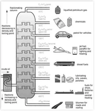
The equipment used for distillation is called a distillation column. Distillation columns
The crude oil, known as the feed, enters the column at a certain stage. The feed may
contain more than one stream in vapor, liquid, or a vapor-liquid combination. In the
column, liquid flows from top to bottom stage by stage. Vapor flows upwards. At each
distillation stage, vapor and liquid are in contact and exchange heat. Then the less volatile
components will condense and the more volatile components will evaporate. As a result, a
feed mixture of chemicals can be separated into the more volatile components at the
upper body of a distillation column as vapor and the less volatile components near the
bottom as liquid. Depending on the feed and the purpose of a distillation process, there
may be more than one stream containing different components out of the column. Later in
Figure 2.1: A Distillation Column
2.1.2 Applications of Distillation
Distillation technologies are widely used in industry, laboratories, and medicinal plant.
The application of distillation can be divided into four groups: laboratory scale, industrial
distillation, distillation of herbs for perfumery and medicinal, and food processing [1].
Many common products in our daily life are produced through distillation. Fuels,
alcohol and medicinal alcohol are products with higher purity alcohol and are distilled
from rough raw materials.
2.2 Concept of Robust Design
Robust design (also known as parameter design) is proposed by Taguchi [5] as a
technique to achieve high quality products. To understand the concept of robust design,
we define the term quality first and then illustrate how to improve quality by means of
robust design.
2.2.1 Definition of Quality
Consistent with the manufacturing approach to quality, we define the quality of a product
as its adherence to specification. If we have a performance characteristic t with a target
value τ, any deviation of t from τ causes demunition in the quality of the product. Thus, in
this context, our objective is to keep the value of t as close to the target value τ as possible.
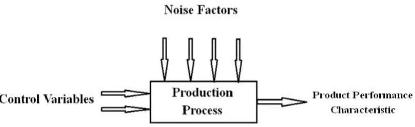
But in a production process usually many factors affect the value of the performance
characteristic t. Figure 2.2 shows a diagram depicting all factors that affect the value of a
performance characteristic (output) t. The inputs to the system are classified as control
variables and noise factors by Taguchi. The control variables are easy to manipulate and
there could be many feasible levels for each of the control variables. On the other hand,
noise factors are difficult or even impossible to control. Some common noise factors
include environmental conditions such as temperature or the atmosphere pressure. The
performance value t is achieved by adjusting the levels for control parameters. Deviations
variation of the noise factors. In this way, the quality for a product depends on the
deviation of the performance characteristic t from the target value τ.
Figure 2.2 Inputs and Output in a Production Process
2.2.2 Fundamentals of Robust Design
Robust design is a technique to improve the quality of a product. As in 2.2.1, the quality
for the product is measured by the deviation of the product’s performance characteristic t
from its target value τ. Both control variable variations and noise factor variations are
sources to cause the deviation in t. In this way, the idea for robust design is to determine
an appropriate set of levels for the control variables so as to minimize this deviation from
a target value without eliminating the noise factors.
2.2.3 Implementations of Robust Design
The technologies to implement robust design can be divided into two categories: design
• Design of Experiment (DOE)
The design of experiment (DOE) approach is less accurate but is widely used to solve
industrial problems. The advantage for DOE is the convenience of implementation and it
is unnecessary to have a closed functional relationship between the performance
characteristic (t) and control parameters. Taguchi and Wu [7] introduced a methodology
of using orthogonal arrays as a DOE approach to robust design problems. The values in
the orthogonal array are the possible levels for each control variable. Taguchi also defined
a performance measure, signal-to-noise ratio (SN ratio), to distinguish robust design
problems.
• Mathematical Analysis
Unlike the first approach, mathematical analysis requires more extensive calculations and
a closed form function of input parameters and performance measurement is necessary.
The result, however, is more accurate than those using DOE technologies as long as the
function is precise.
Some nonlinear programming models are proposed by Box and Fung [8], and Fathi [9].
The Taylor series expansion leads to a nonlinear programming model based on a linear
approximation of the transfer function introduced by Fathi [10].
Monte Carlo Simulation is a simulation method to estimate the mean value and
variance of the product performance characteristic t. Recall that the idea of robust design
is to determine an appropriate set of levels for the control variables so as to minimize the
variables have been decided through DOE or mathematical analysis. By the means of
Monte Carlo simulation, we can determine the mean value, variance, and other
characteristics of the performance measure t.
2.2.4 Applications of Robust Design
Dating back to 1950s, Taguchi and his robust design ideas are widely used in Japanese
companies and quality control associations [5]. In 1980s, robust design is introduced and
promoted in the USA. Some companies including AT&T, Ford, Xerox play important
roles in exposing Taguchi’s idea. A large amount of work has been done to improve this
idea and adapt it to industrial problems. Now the technologies for robust design are
Chapter 3
Binary (two-component) Distillation Column
In this chapter, we apply robust design technologies to a case study based on a binary
distillation column. First, we go through the basic background of a binary distillation
column, describe the case study, and identify control variables and possible noise factors
that would be involved in future analysis. Then we present a mathematical model for the
robust design problem in the case study.
3.1 Introduction to the Binary Distillation Column
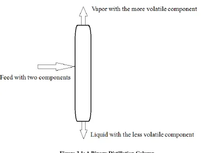
Binary distillation is a special distillation process. It is a multistage process for separating
a mixture of two components [2]. A binary distillation column is shown in Figure 3.1.
Ideally, the less volatile component is separated as vapor and flows out from top. The
more volatile component flows out at bottom as liquid. The product for a binary
distillation process is a pure component, or technically a purer component. The
Figure 3.1: A Binary Distillation Column
3.2 The Case Study
The case is adopted from a pharmaceutical factory [3] with slight modifications. The
factory produces Medicinal Ethanol which has 82.65% of ethanol (mole/mole). The
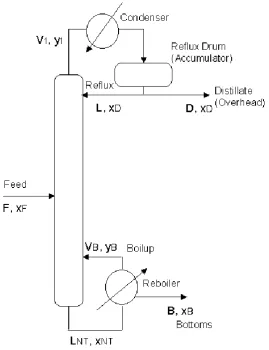
binary distillation column is put into use as shown in Figure 3.2 [13]. There are 40 stages
in the column. We number the stages from top to bottom as 1 to 40, i.e., the top stage is
stage 1 and the bottom stage is stage 40. The feed is a product coming from the upstream
equipment. We use F to represent the feed stream. It enters the column at the kth stage. We
define the feed stage as the stage to enter the feed. In this way, the feed stage is k. The
variable in a more detail later in this chapter. There are two components in the feed:
ethanol and water. As ethanol is more volatile than water, it is vaporized and flows out at
the top of the column, known as V1in Figure 3.2. Then the vapor is fully condensed by a
condenser and then separated through a reflux drum (accumulator) into two streams:
Reflux L and Distillate D. The reflux stream L returns to the column and the distillate
stream D is collected as the product. Meanwhile, water flows downwards and leaves the
system at the bottom, known as flow LNT in Figure 3.2. Then the water is boiled by a
reboiler and separated into Boilup flow VB and Bottoms flow B. VB flows back to the
system and bottoms B is collected as the waste. All the variables and the corresponding
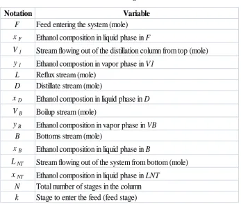
Table 3.1: Variables and According Notations in the Process
Notation Variable
F Feed entering the system (mole) xF Ethanol composition in liquid phase in F
V1 Stream flowing out of the distillation column from top (mole)
y1 Ethanol compostion in vapor phase in V1
L Reflux stream (mole) D Distillate stream (mole)
xD Ethanol compostion in liquid phase in D
VB Boilup stream (mole)
yB Ethanol composition in vapor phase in VB
B Bottoms stream (mole)
xB Ethanol composition in liquid phase in B
LNT Stream flowing out of the system from bottom (mole)
xNT Ethanol composition in liquid phase in LNT N Total number of stages in the column k Stage to enter the feed (feed stage)
3.2.1 The objective for the case study
The pharmaceutical factory in the case is aimed at producing ethanol for medical use. The
desired ethanol composition for the product is 82.65% in mole percentage. There is only
ethanol and water in the binary system and ethanol is more volatile than water. So ethanol
would vaporize and flows out as Distillate D. On the opposite, water flows down and out
of the column as Bottoms B. Then our objective is to keep the ethanol composition in D,
xD, as close to 82.65% as possible. From a robust design perspective, the target value for
the product is τ = 82.65%. The ethanol composition we obtain is the product’s
performance characteristic t = xD. So the objective is to reduce the deviation in xD from
3.2.2 Variables in the Case Study
Which variable in the system can be decided and controlled by us? And which variables
are noise factor disturbing the system? To answer these two questions, we will first divide
the whole system, eliminate unnecessary information and then introduce the role of each
variable.
The feed stage divides the distillation column into two subsystems. The stages above
the feed stage are referred to as the rectifying section. The stages below the feed stage
(including the feed stage) are known as the stripping section. The distillate product is
obtained in the rectifying section. The interactions in the stripping section produce waste
in the bottom and have no direct impact on the rectifying section. So for further analysis,
we will ignore the stripping process and focus on the rectifying section.
Throughout the following chapters, we use y to represent the ethanol composition in
vapor and use x to present the ethanol composition in liquid. For example, if the
composition for ethanol is 0.85 in a vapor flow, then y = 0.85. If the composition for
ethanol is 0.85 in a liquid flow, then x = 0.85. All the compositions are measured in mole
fraction.
3.2.2.1 Control Variables
There are two control variables in the system: the feed stage, and the reflux ratio.
● Feed Stage
The location of the feed stage has a great influence on the whole system. Imagine two
for each component in the distillate would be the same as that in the feed. There was no
product obtained. However, if the feed stage was at the bottom, a great amount of
components would flow out immediately and be wasted. So the feed stage should be set
appropriately to ensure the amount and composition accuracy of the distillate product.
In the case study, there are 40 stages in the distillation column. We assume the feed is
entered at the kth stage. In this way, k is a control variable. The range for k is between 1
and 40. We will explain how to decide the optimal k specifically in the analysis in Chapter
4.
● Reflux Ratio
As discussed earlier in this chapter, back to Figure 3.2, the separated stream V1 is fully
condensed and divided into two streams: reflux L and distillate D. The reflux ratio is a
variable to measure the amount (mole) of reflux L divided by the amount (mole) of
distillate D. We define the reflux ratio as:
(3.1)
R can be controlled by adjusting the settings of the reflux drum. During a distillation
process, the common value for R is set between 1 and 10. How does R affect the system
3.2.2.2 Noise Factors
The temperature for the feed tF is a noise factor to the system. We assume tF is normally
distributed with mean µ = 363.15K, and standard deviation ơ = 0.2K. The temperature for
the feed has an influence on the temperature on each stage. Thus the temperature for the
distillate product is also a random variable. Meanwhile, the composition for each
component (i.e., ethanol and water) depends on the temperature. This relationship is
explained in section 3.2.3. So wherever the temperature is random, the ethanol
composition at that temperature is also random.
3.2.2.3 Relative Volatility
The relative volatility in the system is a dependent random variable. When we have a
mixture of more than one component in a distillation column, the relative volatility of
component p to component q is defined as:
(3.2)
Where x(p) is the composition for component p in the liquid phase and y(p) is the
composition for component p in the vapor phase, and x(q) and y(q) are similarly defined
for component q. In the case of a binary distillation column, we have only two
components, namely, ethanol and water. If we use the notation x to represent the
composition of ethanol in liquid phase and y to represent the composition of ethanol in
respectively. If we further use index i to represent the ith stage (i.e. xi and yi represent the
composition of ethanol in liquid phase and vapor phase, respectively, at stage i), then the
relative volatility at the 1st stage is:
α1 =
(3.3)
And the relative volatility at the feed stage ( the kth stage) is:
αF= αk =
(3.4)
The average volatility for the rectifying section is defined as the average of these two
values above. If we denote the average relative volatility by αA, we have:
(3.5)
3.2.2.4 Pressure in the column
The pressure can be easily controlled and maintained at a desired value. In the case study,
the pressure is assumed to be set at 101.325k Pascal.
3.2.2.5 Other Parameters
In addition to the parameters and variables defined above, we also define a number of
practice, we use xi and yi to represent the ethanol composition for stage i in the liquid and
in the vapor, respectively. Later in section 3.2.3, we describe how these variables depend
on the impact parameter tF. A complete listing of all parameters and variables in our
system is shown in Table 3.2.
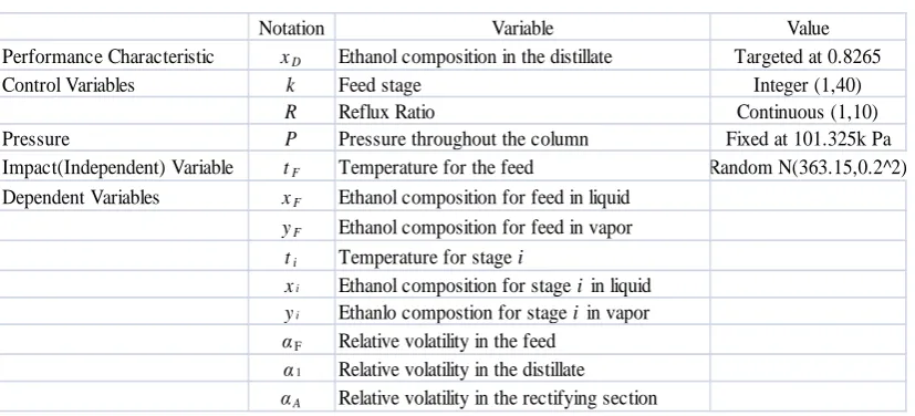
Table 3.2: List of all Parameters and Variables in the System
Notation Variable Value
Performance Characteristic xD Ethanol composition in the distillate Targeted at 0.8265
Control Variables k Feed stage Integer (1,40)
R Reflux Ratio Continuous (1,10)
Pressure P Pressure throughout the column Fixed at 101.325k Pa Impact(Independent) Variable tF Temperature for the feed Random N(363.15,0.2^2) Dependent Variables xF Ethanol composition for feed in liquid
yF Ethanol composition for feed in vapor ti Temperature for stage i
xi Ethanol composition for stage i in liquid
yi Ethanlo compostion for stage i in vapor
αF Relative volatility in the feed
α1 Relative volatility in the distillate αA Relative volatility in the rectifying section
3.2.3 Mathematical Model for the Case
The mathematical model is applied on the rectifying section in the distillation column, for
the product is obtained through this part of the system.
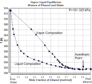
3.2.3.1 Vapor-Liquid Equilibrium Mixture Graph of Ethanol and Water
Vapor-liquid equilibrium is a steady-state for the phases in a vapor-liquid mixture. At this
steady state, the rate of evaporation equals to the rate of condensation. For an ethanol and
water system in the case study, the vapor-liquid equilibrium under pressure 101.325k
separate lines on the graph. Mole fraction of ethanol is graphed on the horizontal axis and
temperature is graphed on a vertical axis. As the temperature goes down, the mole
fraction of ethanol goes up, albeit at different rates for the liquid and the vapor, as shown
in Figure 3.3. At the Azeotropic Point, the liquid composition retains the same value as
the vapor composition.
Figure 3.3: Vapor-Liquid Equilibrium for Ethanol and Water
In order to implement our robust design analysis via a computer simulation model, we use
notation that we defined earlier, we use x to represent the ethanol composition in liquid
phase and y to represent the ethanol composition in vapor phase. Both x and y are
measured in mole fraction (mole/mole). Notice that almost all the temperatures we need
for calculation is between 361K and 364K, so the regression for the analysis is based on
the interval in which T > 361K and T < 364K on the graph. The results are as follows:
For the liquid phase:
x = 3.700 – 0.010 T (360 < T < 364) (3.6)
For the vapor phase:
y = 9.774 – 0.026 T (360 < T < 364) (3.7)
3.2.3.2 Two Equilibrium Equations
With material balance principle and phase equilibrium principle [11], two equations are
deduced as follows:
Phase Equilibrium Equations:
xi = (3.8)
yi =
(3.9)
Equation (3.8) and (3.9) present a relationship between the ethanol composition in vapor
phase at stage i (yi) and the ethanol composition in liquid phase at stage i (xi). Equation
Operation Line Equations:
yi+1 = (3.10)
xi =
(3.11)
Equation (3.10) and equation (3.11) depict the relationship between the ethanol
composition in liquid phase at stage i (xi) and the ethanol composition in vapor phase at
stage (i+1) (yi+1). R is the reflux ratio as defined earlier and it is a control variable. The
value for R is between 1 and 10. According to (3.10), when we know the information for
stage i, xi, we can obtain the ethanol composition for the (i+1) stage yi+1. Equation (3.11)
is the opposite equation for (3.10). For a given yi+1, xi could be calculated through (3.11).
With the two equilibrium equations, we can calculate for the ethanol composition in both
vapor and liquid phase stage by stage. In particular, we have the ethanol composition in
the feed yF and the feed enters at the kth stage. So yF is the value for our variable yk. We
use equation (3.11) to calculate xk-1, and then use equation (3.9) to calculate yk-1. Back to
equation (3.11), we can obtain xk-2. Repeat the procedure to calculate the value of xi and yi
at any stage above the kth stage. In the end, we will reach the ethanol composition y1 for
Chapter 4
Analysis and Solutions
In this chapter, we begin to solve the problem illustrated in the case study. The first
section (4.1) is a general introduction to the simulation procedure. Sections (4.2) and (4.3)
demonstrate the complete simulation for one desired numeral setting. Then by varying the
settings, different results are obtained and presented in section (4.4).
4.1 Introduction to Simulation Procedure
In Chapter 3 we described how to calculate the product performance characteristic xD
through mathematical relationships and equations. How do we carry out a Monte Carlo
Simulation to the case study? How do we set the control variables? How many times does
it need to run the simulation? The answers could be found in this introduction part.
Because there is no closed form function between the input variables (tF etc.) and the
output (xD), we will use Monte Carlo Simulation to solve this robust design problem.
Monte Carlo simulation can achieve high accuracy. Through programming, the results are
direct to view and the settings are easy to change.
We use Excel and Excel VBA to conduct the simulation. Following the calculation
procedures discussed in chapter 3, for a given tF, we first calculate xF and yF under
equation (3.6) and (3.7). Then use equations (3.3) through (3.5) to calculate the relative
control variables R and k, we can obtain the corresponding value of xD. If we repeat the
process for a collection of n randomly generated values of tF, we obtain a random sample
of the corresponding value of xD. We can then determine the mean and standard deviation
of this random sample to estimate the mean and standard deviation of xD. Obviously we
seek a set of values for R and k which achieves the smallest standard deviation for xD
while keeping its mean value equal to the target value 0.8265.
4.2 Possible Combinations for R and k
It seems that R and k can be any value as long as R is between 1 and 10 and k is an integer
between 1 and 40. However, not every combination of R and k is feasible, since we need
to achieve the target value τ = 0.8265 for xD, the output composition. Also recall that the
two extreme situations, when k = 1, the product we obtained is almost the same with the
feed material, and when k = 40, most of the feed material would flow out as waste. To
eliminate the infeasible combinations and make the calculation process quickly, we
evaluate the mean value of xD for every combination of R and k when the independent
random variable tF is at its mean value 363.15K. The set of values for R and k, under
which xD is at its target value 0.8265, is the feasible setting for the system and is used for
calculation illustrated later in section 4.3.
In order to determine these feasible settings for R and k, we use equation (3.8) through
(3.11) as described above. For each value of k, we determine the corresponding value of R
by trial and error; we start at a relatively low value for R (say R = 1.0) and increase this
corresponding value of xD through equation (3.8) through (3.11), and then determine the
value of R that results in xD equal to its target value τ = 0.8265. The feasible values we
obtain in this manner are depicted in Table 4.1.
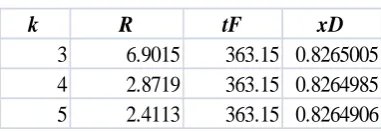
Table 4.1: Feasible Settings for R and k
k R tF xD
3 6.9015 363.15 0.8265005 4 2.8719 363.15 0.8264985 5 2.4113 363.15 0.8264906
Notice that all feasible feed stages are less than 6. This is because the mathematical model
for the system is deduced assuming an ideal system. This value need to be adjusted when
the model is put into practice. We discuss this issue in Chapter 5.
4.3 Minimize Standard Deviation for xD
From section 4.2, only at stage 3, 4, and 5, it is possible to obtain the desired product. So
in the experiment in this section, we will fix the stage at 3, 4, or 5. Then for each stage,
we determine the set point (mean) for R around the given value of R in Table 4.1. For
each combination of values of k and the mean of R we run the Monte Carlo Simulation
method, with sample size n = 1000. We increase the set point by a step size of δ =
0.00001 and repeat the simulation to estimate the corresponding value of the mean and
standard deviation of xD. We then report the value of the set point for R that achieves the
smallest value for the standard deviation of xD while keeping its mean equal to τ = 0.8265.
included in Appendix A.
Table 4.2: Result under Different k
Mean(xD) Standard Deviation(xD)
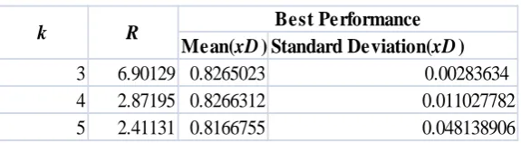
3 6.90129 0.8265023 0.00283634 4 2.87195 0.8266312 0.011027782 5 2.41131 0.8166755 0.048138906
Best Performance
k R
The best performance (Mean of xD is 0.826502 and standard deviation of xD is
0.00283634) is achieved at R = 6.90129 and k = 3. However, if we use 4th stage to enter
the feed, the standard deviation of xD goes up but the reflux ratio R drops down. This is
more obvious when k = 5.
Based on the best performance we achieved at each possible stage (3th stage, 4th stage, and
5th stage), we will illustrate the result in Figure 4.1 and Figure 4.2 to discuss the
Figure 4.1: The Relationship between Standard Deviation of xD and the Feed Stage k
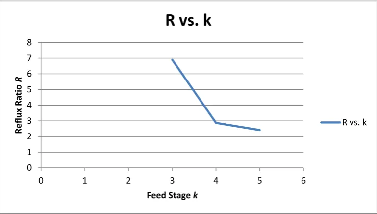
Figure 4.2: The Relationship between Reflux Ratio R and the Feed Stage k
Figure 4.1 depicts the relationship between the feed stage k and the smallest standard
0.00 0.01 0.02 0.03 0.04 0.05 0.06
0 2 4 6
Stan d ar d D e vi ation σxD
Feed Stage k
Standard Deviation vs. k
Standard Deviation vs. k
0 1 2 3 4 5 6 7 8
0 1 2 3 4 5 6
R e fl u x R atio R
Feed Stage k
R vs. k
becomes larger. From stage 4 to stage 5, σxD increases more rapidly.
Then we graphed k and the corresponding R on the same graph in Figure 4.2. From
k = 3 to k = 4, R goes down from 6.9 to 2.9. Then R continues to drop slightly at k = 5.
Recall that R is a ratio of the amount of Reflux (mole) and the amount of Distillate (mole).
So if R is large, a greater portion of the product will flow back to the system to be reused.
The advantage for a small R is to achieve a higher production rate. From this perspective,
stage 4 and stage 5 can both be used to enter the feed in order to obtain a higher
production rate. On the other hand, back to Figure 4.1, if the feed stage is 4 or 5, the
product we obtain would not be in a good quality. The best performance is achieved when
k = 3.
How to determine k and the corresponding R is an essential issue in the whole system. It
depends on the different production requirements. According to the values given in Table
4.1 and 4.2, it appears that k = 4 and R = 2.87195 is a reasonable solution for the problem,
since it is a compromise between having the quality (relatively small value of σxD) and the
production rate (relatively low value for R). This is a potential topic deserving further
analysis and will be discussed in Chapter 5.
4.4 Results under different settings
The settings for the previous example are: total experiment times = 1000, step size δ=
0.00001, and tF ~ N(363.15, 0.22). In this section, we compare different results by
4.4.1 Change experiment times
Suppose we change the total experiment times to 100, 1000, 2000, and 5000, the results
under different settings are displayed in Table 4.3. The step of R and distribution of tF
remain the same.
Table 4.3: Results under Different Experiment Times
Mean(xD) SD(xD)
100 0.8265033 0.00278564 6.90193 3
1000 0.8265023 0.00283634 6.90129 3
2000 0.8264996 0.00287021 6.90211 3
5000 0.8265000 0.00290647 6.90102 3
Experiment Times Best Performance Corresponding R Corresponding k
From Table 4.3, when the experiment times is increased, the mean of xD decreased and
more targeted at 0.8265, but the corresponding standard deviation of xD increased slightly.
Meanwhile, the optimal R is slightly different along with the increment of experiment
times. As we introduced earlier, the product performance characteristic xD is very close to
each other when R is within a small range. The opportunity that a more deviate value
occurs is greater for a relatively large experiment times. However, the more times we run
the simulation, the more accurate result we can obtain.
4.4.2 Change distribution for tF
In this part, we change the standard deviation for tF to 0.01, 0.05, 0.1, and 0.3, keeping
experiment times at 1000 and the step of R at 0.00001. The results are displayed in Table
Table 4.4: Result under Different Standard Deviation for tF
Mean(xD) SD(xD)
0.01 0.8265000 0.00014312 6.90147 3
0.05 0.8265002 0.00073444 6.90089 3
0.1 0.8265005 0.00143529 6.90142 3
0.2 0.8265023 0.00283634 6.90129 3
0.3 0.8264971 0.00435034 6.90073 3
Best Performance
SD for tF Corresponding R Corresponding k
We will conduct a sensitivity analysis on the influence that the standard deviation of tF
(σtF) has on the standard deviation of xD (σxD). Sensitivity analysis is a study to explore the
impact of uncertainty in the input of a model on the uncertainty in model output. In our
example, we use standard deviation to quantity the uncertainty of model input and model
output, σtF and σxD respectively. If the deviation in tF leads to a relatively larger deviation
in xD, xD has a high sensitivity to tF. We use the result in Table 4.6 to illustrate the
sensitivity analysis graphically as shown in Figure 4.3. The standard deviation for tF is
graphed on the horizontal axis and the standard deviation for xD is graphed on a vertical
Figure 4.3: Sensitivity Analysis
The sensitivity that xD has to tF is almost identical along with the change in the standard
deviation of tF (σtF) within the range where σtF < 0.3. The feed stage fixed at 3 and the
reflux ratio R changed slightly. If σtFis larger than 0.3, the regression equations (3.6) and
(3.7) would no longer be valid. It deserves further sensitivity analysis if we modify the
regressions and change σtFin a greater scale.
0.00000 0.00050 0.00100 0.00150 0.00200 0.00250 0.00300 0.00350 0.00400 0.00450 0.00500
0 0.1 0.2 0.3 0.4
Stan d ar d D e vi ation for xD
Standard Deviation for tF
Sensitivity Analysis
Chapter 5
Conclusions and Suggestions for Future Analysis
In this thesis, we have applied robust design principles to a complex distillation process.
Mathematical models and programming simulation are developed to solve the problem.
However, in a realistic production system, future works are strongly recommended to
ensure the operation and system efficiency. There are two essential topics deserving
further analysis: design of production strategy and determination of stage efficiency.
• Design of Production Strategy
The production strategy includes production quantity, operation hours, and cost
minimization etc. In our analysis in the case study, the parameter R is crucial to the final
production quantity. Recall R is defined as the ratio of the amount of reflux stream and the
amount of distillate stream (mole/mole). If R is large, a great portion of product is
refluxed back to the system and the final product we obtained could be much less. So the
value of R should be adjusted to fulfill production requirements. Also, if the time for one
production cycle could be estimated, we are able to decide the operation hours and total
number of equipment accordingly.
It is also a good topic to conduct a cost analysis for this production system. With cost
estimation on the equipment, labor, maintenance, raw material and sales price, we could
and labor arrangement.
• Determination of Stage Efficiency
In our analysis for the case study, we made an important assumption: the vapor and liquid
within the distillation column is at steady state where the rate of evaporation equals to the
rate of condensation and both rates are at desired levels. In practice, there would be some
deviations to the ideal condition. The result is that the rate of evaporation and the rate of
condensation are less than that in the ideal situation. We define the term stage efficiency
as the ratio of the actual evaporation amount to the ideal evaporation amount (mole/mole).
REFERENCES
[1]Wikipedia."Distillation."N.p.,n.d.Web.<http://en.wikipedia.org/wiki/Distillation#Appli
cations_of_distillation>.
[2] Khoury, Fouad M, Multistage Separation Processes. Boca Raton : CRC Press, 2004.
[3] W. Li,"Chemical Process Design Problem Discription." Doc88. N.p., 29 May 2012.
Web. <http://www.doc88.com/p-375363654901.html>.
[4] Phadke, Madhav S, Quality Engineering Using Robust Design. Englewood Cliffs,
N.J. : Prentice Hall, 1989.
[5] Nair, Vijayan N, "Taguchi's Parameter Design: a Panel Discussion", Technometrics 34,
No.2 (1992): 127-161.
[6] Wikipedia, "Vapor-Liquid Equilibrium Mixture of Ethanol and Water." N.p., n.d.
Web.<http://en.wikipedia.org/wiki/File:Vapor-Liquid_Equilibrium_Mixture_of_Ethan
ol_and_Water.png>.
[7] Taguchi, G., and Y. Wu, "Introduction to Off-line Quality", Central Japan Quality
Control Association,1980.
[8] Box, G.E.P., and C.A. Fung, "Studies in Quality Improvement: Minimizing the
Transmitted Variation by Parameter", Center for Quality and Productivity
Improvement , Madison, Wisconsin,1986.
[9] Fathi, Yahya, "A Nonlinear Programming Approach to the Parameter Design Problem",
European Journal of Operational Research 53, No.3 (1991): 371-381.
European Journal of Operational Research 97,No.3 (1997): 561-570. Print.
[11] Smith, Cecil L. Distillation Control: An Engineering Perspective. John Wiley &
Sons, Inc., 2012. WILEY ONLINE LIBRARY. Web.
<http://onlinelibrary.wiley.com/book/10.1002/9781118260050>.
[12] Wikipedia."Relative Volatility."N.p.,n.d.Web.
<http://en.wikipedia.org/wiki/Relative_volatility >.
Appendix A – Complete Results for Table 4.2
k Possible R Mean(xD) Sigma(xD)
3 6.9006 0.8266846 0.00284539
6.90061 0.8265185 0.00304423
6.90062 0.8263808 0.00287056
6.90063 0.8265996 0.00291695
6.90064 0.8265627 0.00296901
6.90065 0.8264906 0.00290733
6.90066 0.8264463 0.00299050
6.90067 0.8264107 0.00287073
6.90068 0.8266795 0.00289698
6.90069 0.8264008 0.00304367
6.9007 0.8265779 0.00283660
6.90071 0.8265612 0.00300656
6.90072 0.8265126 0.00286796
6.90073 0.826615 0.00291972
6.90074 0.8264602 0.00304842
6.90075 0.8264703 0.00284562
6.90076 0.8266689 0.00291931
6.90077 0.8266114 0.00293740
6.90078 0.8264522 0.00284427
6.90079 0.8265484 0.00286716
6.9008 0.8265227 0.00295131
6.90081 0.8266661 0.00292263
6.90082 0.8265453 0.00287914
6.90083 0.8265957 0.00301386
6.90084 0.8265137 0.00290993
6.90085 0.82658 0.00279885
6.90086 0.8265939 0.00286201
6.90087 0.8264665 0.00287520
6.90088 0.8264171 0.00291091
6.90089 0.8264344 0.00288057
6.9009 0.8264795 0.00284764
6.90091 0.8266543 0.00291346
6.90092 0.8265927 0.00286142
6.90093 0.8265603 0.00288466
6.90094 0.8264016 0.00303019
6.90095 0.8264975 0.00286239
6.90096 0.8266243 0.00289583
6.90097 0.8265838 0.00305847
6.90098 0.8263609 0.00294817
6.90099 0.8265583 0.00287777
6.901 0.8266062 0.00281251
6.90101 0.8266285 0.00285681
6.90102 0.8263718 0.00294027
6.90103 0.8266859 0.00299049
6.90104 0.8262986 0.00297095
6.90105 0.8266485 0.00285169
6.90106 0.8265399 0.00287974
6.90107 0.8265299 0.00285789
6.90108 0.8263192 0.00294705
6.90109 0.826617 0.00282720
k Possible R Mean(xD) Sigma(xD)
k Possible R Mean(xD) Sigma(xD)
k Possible R Mean(xD) Sigma(xD)
4 2.87186 0.8259138 0.0114619 2.87187 0.8259699 0.0117849 2.87188 0.8258231 0.0108961 2.87189 0.8254856 0.011279 2.8719 0.8258717 0.0109903 2.87191 0.8261343 0.0116191 2.87192 0.8260526 0.0114653 2.87193 0.8261378 0.0112863 2.87194 0.8254751 0.0110952 2.87195 0.8266312 0.0110278 2.87196 0.8250616 0.0115926 6.90071 0.9495685 0.123071
k Possible R Mean(xD) Sigma(xD)