Simple methods for testing the molecular evolutionary clock hypothesis.

(1)

Simple Methods for Testing the Molecular Evolutionary Clock Hypothesis

Fumio Tajima

Department of Population Genetics, National Institute of Genetics, Mishima, Shizuoka-Ken 41 1, Japan Manuscript received February 15, 1993

Accepted for publication June 17, 1993

ABSTRACT

Simple statistical methods for testing the molecular evolutionary clock hypothesis are developed which can be applied to both nucleotide and amino acid sequences. These methods are based on the chi-square test and are applicable even when the pattern of substitution rates is unknown and/or the substitution rate varies among different sites. Furthermore, some of the methods can be applied even when the outgroup is unknown. Using computer simulations, these methods were compared with the likelihood ratio test and the relative rate test. The results indicate that the powers of the present methods are similar to those of the likelihood ratio test and the relative rate test, in spite of the fact that the latter two tests assume that the pattern of substitution rates follows a certain model and that the substitution rate is the same among different sites, while such assumptions are not necessary to apply the present methods. Therefore, the present methods might be useful.

W

HETHER the molecular evolutionary clock hypothesis (ZUCKERKANDL and PAULINC 1965) holds or not is one of the most important issues in molecular evolution [e.g., see KIMURA (1983)l. This hypothesis may not hold if natural selection is oper- ating, or if mutation rate is not constant per year.

Although there are several methods for testing this hypothesis, all methods have some problems. (i) Ab- solute rate of molecular evolution cannot be estimated unless we know the divergence time. (ii) We must know the pattern of substitution rates to estimate the number of nucleotide (or amino acid) substitutions per site. (iii) We must also know the variation of substitution rates among different sites to estimate the number of substitutions per site. (iv) T h e phylogenetic relationship among nucleotide (or amino acid) sequences must be known before the test is performed. T h e relative rate test (SARICH and WILSON 1967; WU and LI 1985) and the likelihood ratio test (MUSE and WEIR 1992) have overcome the first problem, but still have the other problems. WU and LI’S (1 985) test assumes that the pattern of substitution rates follows KIMURA’S (1980) substitution model, and MUSE and WEIR’S (1992) test assumes more sophisticated substitution models. However, we usually do not know whether these substitution models are correct, although they may be good approximations in some cases. T h e third problem is more difficult to overcome. Although it may be possible to assume that the substitution rate varies from site to site according to some specific distributions such as the gamma distribution

UIN

and NEI 1990; LI et al. 1990), it is not clear whether such an assumption significantly im- proves the test. In order to conduct the relative rate test and the likelihood ratio test, the phylogenetic

Genetics 1 3 5 599-607 (October, 1993)

relationships among three sequences must be known. For example, the phylogenetic relationships among eutherian mammals are controversial (EASTEAL 1990; GRAUR, HIDE and LI 1991; NOVACEK 1992). If the phylogenetic relationships assumed were wrong, we would obtain the wrong conclusion.

In this report I shall present methods for testing the molecular evolutionary clock hypothesis, which overcome the above problems. These methods are so simple that they can be easily applied to any nucleotide (or amino acid) sequences as long as alignment is possible.

THEORY

Suppose that we have three nucleotide sequences, say sequences 1, 2 and 3, which are already aligned, and consider only the sites without gaps. Let nyh be the observed number of sites where sequences 1, 2 and 3 have nucleotides i, j and

k,

respectively. T h e subscripts i, j and

k

take the values 1, 2, 3 and 4 for nucleotides A, G , C and T, respectively.

Case where the outgroup is known: We assume that sequence 3 is the outgroup. Then, the expectation of nGk must be equal to that of njih, i.e.,

E(%jk) = E(njih), (1)

whatever the substitution model is, and even if the substitution rate varies among different sites. If this equality does not hold, we can conclude that the rate is not constant per year. This is the basis of the present method.

(2)

number of sites in which nucleotides in sequence 1 are different from those in sequences

2

and 3 by m l . In the same way we define m2 and m3. Namely, we define m l , m2, and m3 as follows:

ml =

CC

nqj ( 2 4

m2 =

CC

njq (2b)

m3 = CC n,ji ( 2 4

i j t i

t ]#I

i j#i

When sequence 3 is the outgroup, it is clear from (1) that the expectation of ml must be equal to the expectation of m2, i.e.,

E ( m l ) = E(m2). (3)

This equality can be tested by using chi-square. Namely,

x 2 = (ml

-

m2)'

approximately follows the chi-square distribution with one degree of freedom (1 d.f.), noting that the expectations of m l and m2 are both ( m l

+

m2)/2 when ml

+

m2 is given. I call this method one-degree-of-freedom method (1D method). Another derivation of ( 4 ) is given in the APPENDIX.

For example, when ml = 50 and m2 = 30, we have

x2

= (50

-

30)'/(50

+

30) = 5 . 0 0 0 and

P(x'

2 3.841)

12334

+

12443, ( 5 4

v 3 = m3

-

s3. ( 5 f )

When sequence 3 is the outgroup, it is clear that E(s1) = E ( s z ) and E ( v l ) = E(vg), and that

from (1)

(6)

20)*/(5

+

20) = 9.0 for 2DN method (significant at the 5% level).

T h e reason why the 1DN method is appropriate as a statistical test is as follows. Suppose that mp I m3 5

m l , and that there is a significant difference between m2 and m 3 . There are three possibilities in terms of outgroup. (i) If the true outgroup is sequence 1, then this test is the same as the 1 D method. Therefore, we reject the molecular evolutionary clock hypothesis. (ii) If the true outgroup is sequence 3 , then m2 is significantly different from ml because of m3 5 ml. There- fore, we reject the hypothesis. (iii) If the true outgroup is sequence 2, then the substitution rate in the lineage leading to the outgroup sequence is significantly slower than that in the lineages leading to the other two sequences. Therefore, we reject the hypothesis. In all the cases w e reject the hypothesis, so that this method is appropriate as a statistical test.

(3)

Test of Molecular Clock Hypothesis

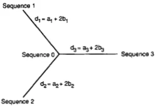
Sequence 1

/

d,= %+ 2 4 Sequence 2

FIGURE 1 .-Phylogenetic relationship among three sequences used for computer simulations.

method is applicable. As will be shown in the next section, results of computer simulations suggest that this method is also applicable.

COMPUTER SIMULATION

In order to know whether the present methods are appropriate as statistical tests, as well as to know the powers of the tests, I have conducted computer simulations.

Substitution model:

I

used KIMURA’S (1 980) substitution model to generate sequence data. Let P g ( t ) be the probability that a site originally having nucleotide

i is occupied by nucleotide j after a time t. T h e subscripts i and j take the values 1, 2, 3 and 4 for nucleotides A, G, C and T, respectively, as before. T h e substitution rates are defined by P 1 2 ( d t ) = P z l ( d t ) = P34(dt) = P43(dt) = adt for transitional changes and

= P4,(dt) = P42(dt) = Odt for transversional changes. Then, P l j ( t ) ’ s are given by

P13(dt) = Pl4(dt) = P23(dt) = P24(dt) = P J l ( d t ) = PJB(dt)

P,,(t) = - 1+ - 1e-48t +

-

1 e-2(a+8)I

4 4 2

for no change, ( 7 4

for transition, (7b)

p,(t) =

-

1

-

1 e-481

4 4 for transversion, (7c)

where i # j . I used the phylogenetic tree in Figure 1, where sequence 3 is assumed to be the outgroup. For simplicity, at and Pt for the lineage leading to sequence i are defined to be a; and b,, respectively. T h e number of nucleotide substitutions per site ( d ) is given by at

+

28t, so that the number of substitutions per site (d,) in the lineage leading to sequence i is given by ai

+

26,.

First, I generated sequence 0 by assuming that each site is occupied by one of four nucleotides with equal probability. Then, sequences 1, 2 and 3 were generated, according to the above probabilities. Finally, chi-

square values for four methods were computed from m,, si and vi

(i

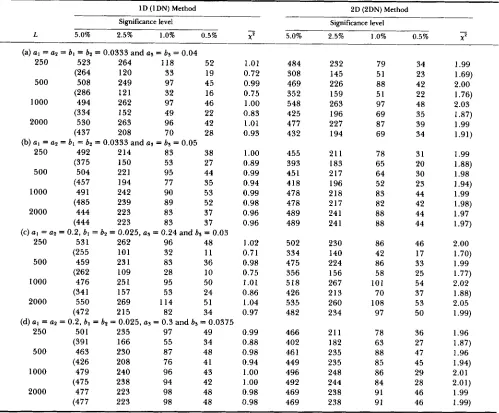
= 1, 2 and 3). T h e length of nucleotide sequence ( L ) is 250, 500, 1000 or 2000, and the number of replications is 10,000 for each set of parameter values.

Distribution of test statistic: In order to confirm that the present methods are appropriate, the distributions of test statistics for several sets of parameter values were examined. T h e results of computer simulation are shown in Tables 1 and 2, where the numbers of replications which were rejected at partic- ular significance levels given together with the aver- ages of chi-square values.

Parameter sets (a) and (b) in Table 1 assume that the rate of transitional substitution is the same as that of transversional one, whereas parameter sets (c) and (d) assume that the rate of transitional substitution is eight times higher than that of transversional one. T h e lineage leading to the outgroup sequence (sequence 3) is 1.2 times longer than the lineages leading to sequences 1 and 2 in the cases of (a) and (c), whereas it is 1.5 times longer in the cases of (b) and (d). We can see from this table that the distributions of chi- square values obtained by using the 1 D and 2D methods are close to their expectations, and that the aver- ages of chi-square values are not significantly different from their expectations, i.e., one and two for the 1D and 2D methods, respectively. Therefore, we can conclude that these methods are appropriate. On the other hand, the 1DN and 2DN methods tend to give smaller chi-square values than do the I D and 2D methods, especially when the outgroup lineage is short and when the length of sequence ( L ) is short. This means that the 1DN and 2DN methods are appropriate although they are conservative. Therefore we can conclude that these methods are useful when the outgroup is unknown.

Table 2 gives the distributions of chi-square values when the pattern of substitution rates in the outgroup lineage is different from that in the t w o other lineages. In this case the substitution rate in the lineage leading to sequence 1 is the same as that of sequence 2. This table shows that chi-square values obtained by using the 1D and 2D methods are close to their expectations, so that we can conclude that these two methods are appropriate. Chi-square values obtained by using the 1DN method tend to be smaller than those of the 1 D method when the outgroup lineage is short and when the length of sequence ( L ) is short, as in Table

(475 238 94 42 1

.oo

2000 477 223 98 48 0.98

(477 223 98 48 0.98

(c) G I = a2 = 0.2, bl = b2 = 0.025, as = 0.24 and b, = 0.03

(d) a1 = a2 = 0.2, bl = b2 = 0.025, as = 0.3 and bs = 0.0375

484 308 469 352 548 425 477 432 455 393 45 1 418 478 478 489 489 502 334 475 356 518 426 535 482 466 402 46 1

449 496 492 469 469 232 145 226 159 263 196 227 194 211 183 217 196 218 217 241 241 230 140 224 156 267 213 260 234 21 1 182 235 235 248 244 238 238 79 51 88 51 97 69 87 69 78 65 64 52 83 82 88 88 86 42 86 58 101 70 108 97 78 63 88 85 86 84 91 91 34 23 42 22 48 35 39 34 31 20 30 23 44 42 44 44 46 17 33 25 54 37 53 50 36 27 47 45 29 28 46 46 1.99 1.69) 2.00 1.76) 2.03 1.87) 1.99 1.91) 1.99 1.88) 1.98

1 .94) 1.99 1.98) 1.97 1.97) 2.00 1.70) 1.99 1.77) 2.02 1.88) 2.05 1.99) 1.96 1.87) 1.96 1.94) 2.01 2.01) 1.99 1 .99)

of substitution rates among lineages. For example, in parameter set (a) we reject the hypothesis in about 22% and 33% of cases at the 1% and 5% levels, respectively, when L = 250.

In this study, when the pattern of substitution rates is different among lineages, we assume that the molecular evolutionary clock hypothesis does not hold even if the overall substitution rate is the same among lineages, since neither the transitional nor transversional substitution rate is constant. Furthermore, it might be very unlikely that the overall rate is constant when the transitional and transversional rates are different. Therefore, it might not cause any serious problem.

Power of statistical test: In order to know the power of the statistical test, I have conducted computer simulations. T h e results are given in Table 3, where the transitional rate was assumed to be equal

to the transversional rate. T h e results obtained by using the 1D method are shown together with those obtained by MUSE and WEIR (1992). T h e 1D method appears to be slightly more powerful than the likelihood ratio test (LR) of MUSE and WEIR (1992) and the relative rate test (WL) of Wu and LI (1985). In these sets of parameter values, the power of the 1DN method was essentially the same as that of the 1D method.

(5)

Test of Molecular Clock Hypothesis 603

TABLE 2

Distribution of test statistic when the pattern of substitution rates in the outgroup lineage is different from that in the lineages leading to the other two sequences

1 D (1 DN) Method 2D (2DN) Method

Significance level Significance level

L 5.0% 2.5% 1.0% 0.5%

-

X 2 5.0% 2.5% 1.0% 0.5% X*

-

(a) a, = ae = bl = bp = 0.0833, as = 0.24 and bs = 0.03

250 488 242 98 56 0.99 46 1 220 77 33 1.99

(173 67 23 13 0.67 3330 280 1 2193 1793 5.29)

1000 483 243 94 49 0.98 477 244 99 45 1.97

(305 128 49 20 0.79 2716 2578 2499 2467 10.58)

250 487 22 1 83 41 0.99 483 233 84 37 1.99

(365 142 41 19 0.88 1322 992 713 563 2.96)

1000 493 264 110 56 1.01 499 244 9 3 60 2.01

(485 258 108 52 1.01 554 304 155 122 2.25)

250 507 254 113 62 1

.oo

529 259 110 52 2.03

(353 182 66 34 0.86 1732 1414 1111 903 3.52)

1000 501 246 90 52 1

.oo

476 229 88 49 1.99

(b) a1 = a p = bl = b p = 0.0833, as = 0.3 and bs = 0.0375

(c) a1 = a2 = 0.2, b1 = bp = 0.025 and as = bn = 0.1

(483 230 83 48 0.99 597 361 238 191 2.54)

250 490 235 88 43 0.99 476 218 81 38 1.99

(468 224 79 37 0.97 660 393 23 1 170 2.20)

1000 489 227 96 47 0.98 493 259 99 50 1.97

(489 227 96 47 0.98 493 259 99 50 1.97)

(d) al = ap = 0.2, bl = bz = 0.025 and a3 = bs = 0.125

TABLE 3

Power of statistical test for a 5% significance level, where dl = 0.05, ds

=

0.3 and L = 1000 were assumed

Results obtained by using the 1 DN method are the same as those

of the 1D method, except in the case of de = 0.25. In this case 1.0000 (60.38) was obtained by using the IDN method.

Results from MUSE and WEIR (1 992).

and the relative rate test (WL) of Wu and LI (1985). In these sets of parameter values, the powers of the 1DN and 2DN methods were essentially the same as those of the 1D and 2D methods, respectively. It should be noted that, in set 9, the overall rate is the same between sequences 1 and 2 but the transitional and transversional rates are different between them.

From these results we can conclude that the 1 D and 2 D methods are as powerful as those of the likelihood ratio test and the relative rate test, in spite of the fact that the 1 D and 2D methods have no assumption about the pattern of substitution rates.

To investigate the difference between the I D and 1DN methods and that between the 2D and 2DN method, as well as the effect of the choice of outgroup

on the statistical power, I have conducted computer simulations, where the transitional rate was assumed to be two times as high as transversional rate and only the length ( d 3 ) of the lineage leading to the outgroup was changed. T h e results are shown in Table 6. As expected, the powers of the 1D and 2D methods increase as d s decreases, since the outgroup is known under these methods. Therefore, we can conclude that when the outgroup is known, these methods are more powerful when the outgroup lineage is shorter. On the other hand, the 1DN and 2DN methods show different properties. When ds = 0.08 (= d l ) , there is no statistical power. As ds decreases, the power increases. This is because, using these methods, we are actually testing the difference between sequences 1 and 3, not between sequences 1 and 2. As ds increases from 0.08, the power increases, reaches to its maxi- mum value, and decreases. This is because, as d s increases, the probability of making a comparison between sequences 1 and 2 increases.

NUMERICAL EXAMPLE

(6)

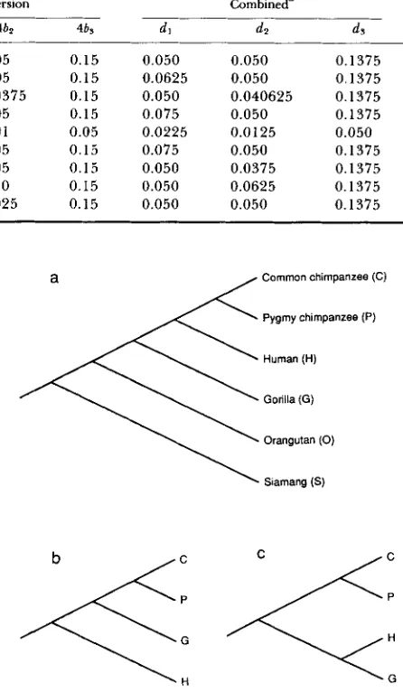
TABLE 4

Parameter values for computer simulations

Transition Transversion Combined’

Set 4a I 4a2 4as 461 461 46s dl d t ds

1 0.10 0.10 0.25 0.05 0.05 0.15 0.050 0.050 0.1375

2 0.125 0.10 0.25 0.0625 0.05 0.15 0.0625 0.050 0.1375

3 0.10 0.0875 0.25 0.05 0.0375 0.15 0.050 0.040625 0.1375

4 0.15 0.10 0.25 0.075 0.05 0.15 0.075 0.050 0.1375

5 0.05 0.03 0.10 0.02 0.01 0.05 0.0225 0.0 125 0.050

6 0.10 0.10 0.25 0.10 0.05 0.15 0.075 0.050 0.1375

7 0.10 0.05 0.25 0.05 0.05 0.15 0.050 0.0375 0.1375

8 0.10 0.05 0.25 0.05 0.10 0.15 0.050 0.0625 0.1375

9 0.10 0.15 0.25 0.05 0.025 0.15 0.050 0.050 0.1375

a d, = a,

+

26,.

TABLE 5

Power of statistical test for a 5% significance level, where parameter values in Table 4 and L 1000 were used

Set

1 2

3

4 5

6

7 8 9

2D

0.0479 0.1305 0.1093 0.3636 0.2666 0.5812 0.2888 0.7300 0.4678

Method LR2Pa 1D

0.044 0.0507

0.1 15 0.1722

0.112 0.1327

0.388 0.4626

0.286 0.3555

0.61 1 0.4802

0.297 0.1925

0.718 0.1787

0.497 0.0515

L R ~ P ~

0.040 0.158 0.129 0.483 0.375 0.497 0.214 0.165 0.049

_ _

w

La

0.041 0.155 0.127 0.472 0.361 0.458 0.215 0.156 0.049

Results obtained by using the 1 DN method are the same as those

of the ID method, and results obtained by using the 2DN method

are the same as those of the 2D method, except in set 5. In this set

0.2665 was obtained by using the 2DN method.

a Results from MUSE and WEIR (1992).

TABLE 6

Power of statistical test for a 5% significance level, where dl =

0.08 (a, = 0.04, b, = 0.02), dt = 0.12 (ar = 0.06, b, = 0.03) and L

= 1000 were assumed

Parameter

a3 b3 dr

0.01 0.005 0.02

0.02 0.01 0.04

0.03 0.015 0.06

0.04 0.02 0.08

0.05 0.025 0.10

0.06 0.03 0.12

0.08 0.04 0.16

0.10 0.05 0.20

0.20 0.10 0.40

0.40 0.20 0.80

0.80 0.40 1.60

1.60 0.80 3.20

Method

2D 2DN I D I DN

0.6473 0.9989 0.7395 0.9997

0.6259 0.8064 0.7307 0.8860

0.6040 0.2275 0.7111 0.2940

0.5859 0.0482 0.6904 0.0491

0.5664 0.1643 0.6740 0.2163

0.5593 0.4026 0.6659 0.5109

0.5144 0.5129 0.6236 0.6219

0.4742 0.4742 0.5785 0.5785

0.3183 0.3183 0.4087 0.4087

0.1489 0.1489 0.1898 0.1898

0.0648 0.0648 0.0704 _0.0794

0.0470 0.0470 0.0468 0.0468

a

,

Common chimpanzee (C) Pygmy chimpanzee (P) Human (H) Gorilla (G)

Orangutan (0)

b C

‘G

FIGURE 2.-Phylogenetic relationships among hominoid species.

oxidase subunits I and I1 (COI and COII), ATPase 8, parts of two genes for ND1 and ATPase 6, and 11 interspersed tRNAs. In order to apply the 1 D and 2D methods, we must know the phylogenetic relationship among these sequences. I used the phylogenetic relationship shown in Figure 2a. T h e relationship among (common and pygmy) chimpanzee, human and gorilla is controversial [e.g., see MARKS (1992)J although HORAI et al. (1992) strongly suggest that of Figure 2a. Therefore, I also used the phylogenetic relationship shown in Figures 2b and 2c for the relationship among these species.

(7)

of Molecular Clock Hypothesis 605

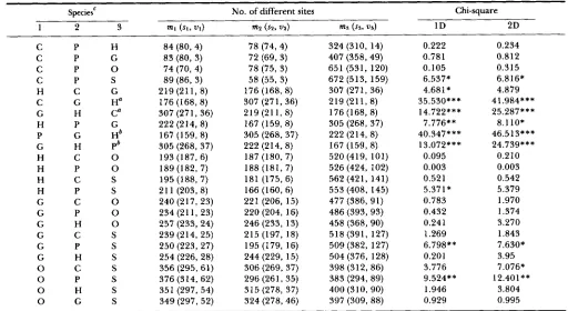
TABLE 7

Testing hominoid mitochondrial DNA sequences

No. of different sites Chi-square

C P H

C P G

C P 0

C P S

H C G

C G Ha

G H C0

H P G

P G Hb

G H P b

H C 0

H P 0

H C S

H P S

G C 0

G P 0

G H 0

G C S

G P S

G H S

0 C S

0 P S

0 H S

0 G S

84 (80, 4) 8 3 (80, 3)

74 (70, 4) 89 (86, 3) 219 (211, 8)

176 (168, 8) 307 (27 1, 36) 222 (214, 8) 167 (159, 8)

305 (268, 37) 193 (187, 6) 189 (182, 7) 195 (188, 7) 21 1 (203, 8) 240 (217, 23) 234 (21 1, 23) 257 (233, 24) 239 (214, 25) 250 (223, 27) 254 (226, 28) 356 (295, 61) 376 (314, 62) 351 (297, 54) 349 (297, 52)

78 (74, 4) 72 (69, 3) 78 (75, 3) 58 (55, 3) 176 (168, 8) 307 (271, 36) 219 (211, 8) 167 (159, 8) 305 (268, 37) 222 (214,8) 187 (180, 7) 188 (181, 7) 181 (175, 6) 166 (160, 6) 22 1 (206, 15) 220 (204, 16)

246 (233, 13) 215 (197, 18) 195 (179, 16) 244 (229, 15) 306 (269, 37) 296 (261, 35) 3 15 (278, 37) 324 (278, 46)

324 (310, 14) 407 (358,49) 651 (531, 120) 672 (513, 159) 307 (271, 36) 219 (21 1, 8) 176 (168, 8) 305 (268, 37) 222 (214, 8) 167 (159,8) 520 (419, 101) 526 (424, 102) 562 (42 1, 141) 553 (408, 145) 477 (386, 91) 486 (393, 93) 458 (368.90) 518 (391, 127) 509 (382, 127) 504 (376, 128) 398 (312, 86) 383 (294, 89) 400 (3 10, 90) 397 (309, 88)

0.222 0.781 0.105 6.537* 4.681* 35.530*** 14.722*** 7.776** 40.347*** 13.072*** 0.095 0.003 0.521 5.37 1

*

0.783 0.432 0.241 1.269 6.798** 0.201 3.776 9.524** 1.946 0.929 0.234 0.812 0.315 6.816* 4.879 41.984*** 25.287*** 8.110* 46.513*** 24.739*** 0.210 0.003 0.542 5.379 1.970 1.374 3.270 1.843 7.630* 3.95 7.076* 12.401** 3.804 0.995

Data from HORAI et al. (1992). Chi-square values obtained by using the 1DN and 2DN methods are the same as those of the 1 D and 2D

a In the cases of CGH and GHC, chi-square values obtained by using the 1DN and 2DN methods are 4.681 * and 4.879, respectively.

In the cases of PGH and GHP, chi-square values obtained by using the 1DN and 2DN methods are 7.776** and 8.1 lo*, respectively.

'

Species 3 was used as the outgroup in the 1 D and 2D methods. Species abbreviations are: C, common chimpanzee; P, pygmy chimpanzee;

*

Significant at 5% level;

**

significant at 1 % level;

***

significant at 0.1 % level.

methods, respectively, except in the cases of CGH, GHC, PGH and GHP.

H, human; G , gorilla; 0, orangutan; and S, siamang.

previous section, the 1D and 2D methods are more powerful when the outgroup is more closely related. Since chi-square values are not significantly large when H , G and 0 were used as the outgroup, the molecular evolutionary clock hypothesis cannot be rejected. In the comparison among H , (C or P) and G, significantly large chi-square values were obtained although the values depend on the choice of outgroup. Since the outgroup is unknown, it might be better to apply the 1DN and 2DN methods. Then, w e have significantly large chi-square values

( x 2

= 4.681 in the comparison among H, C and G for the 1DN method,

and

'

x

= 7.776 and 8.1 10 in the comparison among

H , P and G for the 1DN and 2DN methods), so that the molecular clock hypothesis can be rejected. In the comparison among (H or G), P and S, significantly large chi-square values were obtained. Since chi- square values are not significantly large when the outgroup is 0, we cannot reject the molecular clock hypothesis. When the comparison was made among 0, (C or P) and S, we have significantly large chi- square values

( x 2

= 9.524 for the 1D and 1DN meth- ods, and x' = 7.076 and 12.401 for the 2D and 2DN

methods), so that we can reject the molecular clock hypothesis.

It should be noted that it might be very difficult to apply the likelihood ratio test and the relative rate test to the present data, since the substitution rate varies among different sites. (For example, the substitution rate in tRNAs is different from that in proteins, the rate varies among different proteins, the rate in stem regions of tRNA is different from that in loop regions, the rate varies among different loop regions, and so on.) On the other hand, there is no difficulty in applying the present methods.

DISCUSSION

In this report, simple methods for testing the molecular evolutionary clock hypothesis were developed. In these methods, we do not have to assume a partic- ular pattern of substitution rates. Furthermore, these methods are applicable even when the substitution rate varies among different sites. T h e 1DN and 2DN methods can be used when the outgroup is unknown. Therefore, the present methods might be useful.

(8)

1DN methods, whereas this number is classified into transitional and transversional ones in the 2 D and 2DN methods. T h e number of different sites, however, can be classified into many groups. For example, as a test statistic we can use

with 24 d.f., or

with 12 d.f. Since the 2 D method is not always more powerful than the 1D method, it is not clear whether (8) and (9) are powerful. Although (9) may be useful in some cases, very long sequences must be necessary to conduct the statistical test. It is also possible, when the substitution rate of transition is substantially higher than that of transversion, that only the transitional differences are classified into four classes, i . e . ,

with 5 d.f., although it is not clear how powerful (1 0) is. For example, when we compare mitochondrial sequences from human and common chimpanzee by using gorilla as the outgroup, we have nIz2 = 10, nZ12

= 18, n2t1 = 5 3 , nlzl = 4 3 , n344 = 6 3 , n434 = 3 2 , n433

= 8 5 , 12343 = 7 5 and v1 = v2 = 8. Then, we obtain

x 2

= 14.068 and P ( x 2 L 11.070) = 0.05 for 5 d.f., so that we reject the molecular evolutionary clock

hy-

pothesis at the 5% level. T h e power of (10) probably depends on the pattern of substitution rates, the length of sequence, the divergence time, and so on.

In this paper we consider only nucleotide sequences. It might be clear, however, that we can also apply the present methods to amino acid sequences.

I thank S. HORAI and A. G. CLARK for their suggestions and

comments. This is contribution no. 1966 from the National lnsti- tute of Genetics, Mishima, Shizuoka-ken 41 1, Japan.

LITERATURE CITED

EASTEAL, S., 1990 The pattern of mammalian evolution and the

relative rate of molecular evolution. Genetics 1 2 4 165-173.

GRAUR, D., W. A. HIDE and W. H. LI, 1991 Is the guinea-pig a

rodent? Nature 351: 649-652.

HORAI, S., Y. SATTA, K. HAYASAKA, R. KONDO, T. INOUE, T.

ISHIDA, S. HAYASHI and N. TAKAHATA, 1992 Man's place in

Hominoidea revealed by mitochondrial DNA genealogy. J.

Mol. EvoI. 35: 32-43.

JIN, L., and M. NEI, 1990 Limitations o f the evolutionary parsi-

mony method of phylogenetic analysis. Mol. Biol. Evol. 7: 82-

102.

KIMURA, M., 1980 A simple method for estimating evolutionary

rate of base substitutions through comparative studies of nucleotide sequences. J. Mol. Evol. 16: l 11-120.

KIMURA, M., 1983 The Neutral Theory of Molecular Evolution.

Cambridge University Press, Cambridge.

LI, W. H . , M. GOUY, P. M. SHARP, C . O'HUIGIN and Y. W. YANG, 1990 Molecular phylogeny of Rodentia, Lagomorpha, Pri- mates, Artiodactyla, and Carnivora and molecular clocks. Proc.

Natl. Acad. Sci. USA 87: 6703-6707.

MARKS, J., 1992 Genetic relationships among the apes and hu-

MUSE, S. V . , and B. S. WEIR, 1992 Testing for equality of evolu-

NOVACEK, M. J., 1992 Mammalian phylogeny: shaking the tree.

SARICH, V. M., and A. C. WILSON, 1967 Immunological time scale

WU, C. l . , and W. H. LI, 1985 Evidence for higher rates of nucleotide substitution in rodents than in man. Proc. Natl.

Acad. Sci. USA 82: 1741-1745.

mans. Curr. Opin. Genet. Dev. 2: 883-889.

tionary rates. Genetics 132: 269-276.

Nature 356: 121-125.

for hominid evolution. Science 158: 1200-1203.

ZUCKERKANDL, E., and L. PAULING, 1965 Evolutionary divergence

and convergence in proteins, pp. 97-1 66 in Evolving Genes and

Proteins, edited by V. BRYSON and H. J. VOGEL. Academic Press, New York.

Communicating editor: A. G . CLARK

APPENDIX

from the same data, so that the degree of freedom is one. Thus, we obtain ( 4 ) .

L can be divided into sl, s2, '01, vp and L

-

s1

-

sp

-

V I

-

up. Since E(s1) = E(s2) and E(v1) = E ( v ~ ) , we have

r)L, where the unbiased

estimates of q and r are (SI

+

s 2 ) / L and ( v l

+

v2)/L,

(9)

mated by ( S I

+

4 / 2 ,

E ( u l ) and E(u2)

by

(ul

+

v2)/2,

up. Following the definition of chi-square, we have

There are five categories and we estimate q and r from the same data, so that the degree of freedom is

two. Thus, w e obtain (6).