Sequential Change Point Detection.

(1)

ABSTRACT

ZHOU, MI. Sequential Change Point Detection. (Under the direction of Dr. Huixia Judy Wang.)

In this dissertation, we study several sequential change point detection problems in different setups. In Chapter 2, we focus on sequential change point detection in linear quantile regression. We develop a subgradient-based CUSUM-type test statistic for de-tecting change points at a single quantile level or at multiple quantiles and establish the asymptotic properties of the proposed test statistic. Through simulation study we demonstrate that our proposed test can control Type I error better than existing meth-ods.

Chapters 3 and 4 are both motivated by the study of Atlantic basin hurricane count data. Chapter 3 focuses on the detection of change points in generalized linear models. To improve the performance of the asymptotic method for data with small sample sizes, we develop a bootstrap procedure, establish the asymptotic properties and demonstrate the finite-sample advantage of the bootstrap procedure through simulation. At last, we apply the method to the hurricane count data to detect changes in the association of hurricane counts and years.

(2)

c

(3)

Sequential Change Point Detection

by Mi Zhou

A dissertation submitted to the Graduate Faculty of North Carolina State University

in partial fulfillment of the requirements for the Degree of

Doctor of Philosophy

Statistics

Raleigh, North Carolina 2014

APPROVED BY:

Dr. Lian Xie Dr. Wenbin Lu

Dr. Xinge Jessie Jeng Dr. Huixia Judy Wang

(4)

DEDICATION

(5)

BIOGRAPHY

(6)

ACKNOWLEDGEMENTS

I would like to express my deepest gratitude to my advisor Dr. Huixia Judy Wang for her patience, motivation, enthusiasm and immense knowledge. Her great guidance, encour-agement and support helped me in all the time of research, writing of the dissertation and job seeking. Besides research, she set a great example to us with her dedication to work, self-motivation, time management skills and perfect balance of life and work. I could not have imagined having a better advisor and mentor for my Ph.D. study.

I owe my sincere gratitude to Dr. Lian Xie, for serving on my Ph.D. committee member, for his inspiring discussions that motivated the problems in this dissertation and for his guidance. His ways of critical thinking helped me improve my research.

I thank Dr. Wenbin Lu, Dr. Xinge Jessie Jeng and Dr. Arnab Maity for serving on my Ph.D. committee and for their encouragement and valuable suggestions for this research. I thank Dr. Daowen Zhang for being my academic advisor during my first two years of study at NCSU, and for his encouragement and support.

I would also like to thank Dr. Sujit Ghosh, Dr. Kim Weems and Dr. Howard Bondell for their understanding, encouragement and support during my study in NCSU.

I am also grateful for the staff in the department, especially Alison McCoy, Adrian Blue, David Churchill, Terry Byron, Chris Waddell for their dedication in their work. They set great examples to our students.

Special thanks to all my good friends who shared laughs and tears with me in all these five years.

Last but not least, none of this would have been made possible without my family. I thank my parents and my husband for their unconditional love, and thank my son Andy for perfecting my life.

(7)

LIST OF TABLES

Table 2.1 Asymptotic critical values of Qτ for the open-end procedure at τ = 0.5 with p= 2. . . 14 Table 2.2 Type I errors of the proposed closed- and open-end median procedures

in Case 1 with γ = 0,0.25 and 0.4. The nominal significance level is 0.05. 15 Table 2.3 Summary statistics of the distribution of detection time for different

values of γ = 0,0.25 and 0.4 for the proposed closed-end procedure at median in Case 1 with Tm = 100 and δ= 2. The k∗ represents the true change point time. . . 17 Table 2.4 Type I errors (the proportions of rejections underH0) of different

meth-ods in Case 1 with γ = 0.25. The 95% CIs for Type I errors of level-5% and level-10% valid tests are [0.0422,0.0578] and [0.0893,0.1107], re-spectively. . . 20 Table 2.5 Type I errors (the proportions of rejections underH0) of different

meth-ods in Case 4 with γ = 0.25. The 95% CIs for Type I errors of level-5% and level-10% valid tests are [0.0422,0.0578] and [0.0893,0.1107], re-spectively. . . 23 Table 2.8 Asymptotic critical values of the statistic MQ acrossτ ∈[ω,1−ω] with

the number of regressors p = 2 for γ=0, 0.25 and 0.4, and nominal level α = 0.05 and 0.1. The results are based on 50,000 Monte Carlo replications. . . 32 Table 2.9 Type I errors (the proportions of rejections under H0) of the proposed

multiple-quantile method and median method in Cases 1-4 with γ = 0.25. The 95% CIs for Type I errors of level-5% and level-10% valid tests are [0.0422,0.0578] and [0.0893,0.1107], respectively. . . 34 Table 3.1 The rejection rates of the asymptotic and bootstrap methods in the

lin-ear regression model underH0 and three different alternative hypotheses. 57 Table 3.2 The rejection rate of two methods in Poisson regression models under

(10)

Table 4.1 Comparison of Eθ(N) and ¯Eλ(N) of Mei’s method and the GLRT method for Poisson distribution by controlling the long ARL associated with θ0 = 7 at the pre-specified level L1 800. The standard deviations are given in parentheses. . . 75 Table 4.2 Comparison of Mei’s method and the GLRT method of Lorden (1971)

for negative Binomial distribution by controlling the long ARL at 400, θ0 = (5,0.8)T. Results are based on 100 simulations. The standard deviations are given in parentheses. . . 78 Table 4.3 Means and variances before and after the year 2005, and p-values for

(11)

LIST OF FIGURES

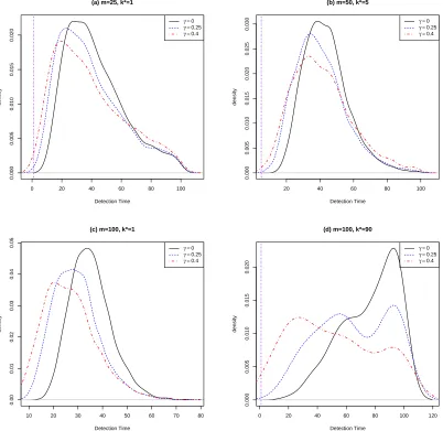
Figure 2.1 The estimated power of the closed-end procedure at median against Tm for different γ values in three cases with m = 50 and δ = 2. The horizontal line represents the 5% nominal level. . . 16 Figure 2.2 The estimated densities of the detection time distribution from the

closed-end procedure at median in Case 1 with Tm = 100, δ = 2 and γ = 0,0.25 and 0.4. The vertical line represents the true change point k∗. . . 18 Figure 2.3 The median detection time against γ for the closed-end procedure at

median in Case 1 with m= 200, Tm = 2m, k∗ = 50 and δ= 2. . . 19 Figure 2.4 The power curves of different methods against the observation

hori-zon Tm in Cases 1-4, where m = 50 and δ = 2. The horizontal line represents the 5% nominal level. . . 24 Figure 2.5 The power curves of different methods against the slope change δ in

Cases 1-4, where Tm = 500 andm= 50. The horizontal line represents the 5% nominal level. . . 26 Figure 2.6 The power curves of different methods (including the modified HHKS

test) against Tm in Case 2, where δ = 2,m = 50 and k∗ = 50. The horizontal line represents the 5% nominal level. . . 27 Figure 2.7 The power curves of different methods against the slope change δ in

Case 2, where Tm = 500 and m = 50. The horizontal line represents the 5% nominal level. . . 28 Figure 2.8 The power curves of the proposed multi-quantile method, the median

method, 25% quantile and 75% quantile methods under the closed-end procedure against δ withm= 200, N = 2 andk∗ = 50. The horizontal dot-dashed line represents the 5% nominal level. . . 35 Figure 3.1 Type I errors of the asymptotic method (—) and the bootstrap method

(- - -) against the nominal level α in the linear regression. The dotted line (· · ·) corresponds to the 45 degree line. . . 56 Figure 3.2 Type I errors of the asymptotic method (—) and the bootstrap method

(12)

Chapter 1 Introduction

1.1 Introduction to Change Point Detection

The problem of testing the structural stability or the consistency of model parameters is usually called change point detection. In some cases when dealing with historical data with a fixed length, we are interested in discovering if one or more structural changes occur at some points in the middle and where they are if they do exist. In other cases when monitoring successive data, it is usually assumed that the data structure stays in a stable state. Once a structural change occurs, we would like to signal the change immediately and thereafter some corrective action can be taken. The change point detection problem can be divided into two categories: retrospective change point detection and sequential change point detection. For the retrospective study, researchers are interested in testing whether a change point or multiple change points exist in the observed data set with a fixed length. For the sequential study, researchers would like to test whether a newly arrived observation is a change point or not. We will focus on the sequential change point detection in this dissertation.

(13)

The sequential change point problem originally arose from statistical quality control and it has been widely applied in other problems, such as fault detection, maintenance of industrial process, safety of complex systems, prediction of natural catastrophic events, finance and monitoring in biomedicine. Extensive studies has been done in these fields in the past few decades; see Basseville and Nikiforov (1993), Lai and Xing (2010) for references.

For the simplest case where f0 and f1 are known, the problem has been well studied. The first proposed scheme was Shewhart’s control chart; see Shewhart (1925). The main idea is to examine samples of a fixed size at regular intervals of time, and compute a test statisticSi of the sample at timei. Then these sequential statistics Si are presented in a chart with control limits. Once a Si falls outside the control limits, the monitoring scheme signals that the process is out of control. Moving average control chart is an alternative monitoring chart, which used a weighted sum of the last few observations as the test statistic; see Page (1954).

The previously mentioned chart schemes are based either on a single point recorded on the control chart or on a fixed number of the recent recorded points. To make use of all the information that is available on the chart, Page (1954) introduced the cumulative sum (CUSUM) schemes. Let Zi be a suitably chosen function or score of the ith sample Xiand let Sn =Pn_i₌₁Zi. A one-sided CUSUM scheme will take action at a stopping time T = inf{n:Sn−min0≤i≤nSi ≥γ}, whereγ is a suitably chosen threshold. In particular, if X1, . . . , Xν−1 are i.i.d.with density f0 and Xν, Xν+1, . . . are i.i.d.with density f1. Let Zi = log{f1(Xi)/f0(Xi)}, then

T = inf "

n : n X

i=1 log

f1(Xi) f0(Xi)

− min 1≤k≤n

k X

i=1 log

f1(Xi) f0(Xi)

≥γ

#

. (1.1)

LetN be the stopping variable that signals that the process is out of control. Lorden (1971) showed the optimality of (1.1) holds asymptotically asγ → ∞, and thatEf1(N)∼

log(γ)/I(f1, f0), where I(f1, f0) = Ef1{f1(X1)/f0(X1)} denotes the Kullback-Leibler

in-formation. Moustakides (1986) and Ritov (1990) showed that the likelihood ratio CUSUM scheme (1.1) is optimal in the sense that (1.1) minimizes sup_ν{(N−ν+1)+_|X

(14)

generalize Page (1954)’s CUSUM scheme to the form

TG = inf "

n : max 1≤k≤n_|_θsup_|≥_γ

n X

i=k log

fθ(Xi) f0(Xi)

≥γ

#

(1.2)

by letting γ ∼ (logγ)−1.This scheme is a refinement of the two-sided CUSUM chart considered by Page (1954), Barnard (1959) and Kemp (1961).

Instead of maximizing the likelihood ratio over|θ| ≥γ in (1.2), Pollak and Siegmund (1985) integrated the likelihood ratio with respect to some probability distribution ofθ, H(θ), and proposed the mixture likelihood ratio scheme

TM = inf "

n : max 1≤k≤n

( Z n

Y i=k

fθ(Xi) f0(Xi)

dH(θ) )

≥γ #

.

Mei (2006) proposed a scheme for the case when the pre-change parameter θ0 is unknown, and also developed a general theory for the case when both the pre-change density fθ0 and the post-change density fθ1 involve unknown parameters.

Bayesian techniques are also used for sequential change point detection. For the case with known pre-change density f0 and post-change density f1, Shiryayev (1978) formu-lated the proof of optimal sequential detection of the change point ν in the Bayesian framework by putting a geometric prior distribution on the unknown change point ν : P(ν=n) = p(1−p)n−1, n= 1,2, . . ., and proposed the stopping rule

Np(γ) = inf ( n: n X k=1 n Y i=k

f1(Xi) (1−p)f0(Xi)

≥γ )

.

Letting Rn = Pn

k=1 Qn

i=k{f1(Xi)/f0(Xi)}, Roberts (1966) modified the rules asN(γ) = inf(n : Rn ≥ γ), which was proven by Pollak (1985) to be asymptotically Bayes risk efficient as p → 0. Later, Bojdecki (1980), Bojdecki and Hosza (1984) provided more discussions on the Bayes rule.

(15)

Consider the linear regression model

yi =xTi βi+i, i= 1,2, . . . ,

where yi is the dependent variable, xi is the p-dimensional predictor,βi is the

p-dimensional unknown regression coefficient andi is the random error. The null hypoth-esis is that β_i =β₀ for all i = 1,2, . . . . The standard sequential change point detection in linear regression models is to assess whether there exists an unknown change point ν inβ_i such that β_i =β₁ 6=β₀ for i=ν+ 1, ν+ 2, . . ., where bothβ₀ and β₁ are unknown regression coefficients.

There exist many work on change point detection for linear models. Brown et al. (1975) introduced a CUSUM test statistic to test the constancy of linear regression relationship over time in the form as

Qr = 1 ˆ σ

r X k+1

Wj, Wj =

yj−xTjbj−1 q

1 +xT

j(xTj−1xj−1)−1xj

, r=k+ 1, . . . , n,

where ˆσ=qPn_j₌_k₊₁W2

j/(n−k) is the estimated standard deviation,k is the dimension of regressors, bj is the least-square estimate of β based on the firstj observations, and n is the total number of observations. Ploberger et al. (1989) proposed a fluctuation test which is directly based on successive parameter estimates rather than recursive residuals. However, the work of Brown et al. (1975) and Ploberger et al. (1989) focused on retrospective studies. For sequential change point detection, Chu et al. (1996) made a “noncontamination” assumption that β_i = β₀ for i = 1, . . . , m on the historical period of length m. To test the regression stability in the “post-historical” period, that is H0 : β_i = β₀, for i = m + 1, . . . versus H1: there exists a ν ≥ m + 1 such that βi 6= β0, for i = ν, ν + 1, . . ., Chu et al. (1996) proposed CUSUM of recursive residuals and the parameter fluctuation. Leisch et al. (2000a) introduced a generalized fluctuation test, which is more sensitive to a change occurring late in the monitoring period. Horv´ath et al. (2004) proposed a method based on the weighted CUSUM of residuals. Aue et al. (2006) considered a linear regression model with heteroscedastic errors, and developed a method based on the squares of prediction errors.

(16)

structural changes in GLM. Xia et al. (2009) proposed two monitoring schemes in GLM: one is based on CUSUM of weighted residuals, and the other is based on the moving sum of weighted residuals.

Most of the literature on change point detection focused on detecting the changes in the mean, for instance, to detect whether µ1 = µ2 = . . . = µn, where µi = E(Xi), i = 1, . . . , n. Some others focused on the changes in variance by testing whether σ2

1 =. . .= σ_n2, where σ_i2 = Var(Xi), i= 1, . . . , n. Carsoule and Franses (1999) proposed a sequential testing approach for testing the structural change in the variance of a time series, based on the work in Chu et al. (1996).

1.2 Introduction to Quantile Regression

One objective of regression analysis is to study the relationship between the response and predicting variables. The traditional regression analysis has focused on studying how the mean function of the response depends on the predictors (covariates). Consider a linear regression model

yi =xTi β+i, i= 1, . . . , n, (1.3) where yi represents the response, xi is the p-dimensional vector of covariates, β is the p-dimensional unknown parameter vector, and i’s are independent random errors with conditional mean zero, i.e.E(i|xi) = 0. Consequently E(yi|xi) = xTi β. For model (1.3), the Ordinary Least Squares (OLS) estimator of β is defined as

ˆ

β = arg min β∈Rp

n X

i=1

(yi−xTi β)2.

Solving the minimization problem gives ˆβ = (xT_x₎−1_xT_y_{, where} _y _{= (y}

1, . . . , yn)T rep-resents then×1 vector of responses and x= (xT

(17)

distribution, e.g.the relationship between the test scores and study hours of students in the lower or upper tails of a class in terms of academic performance.

Koenker and Bassett (1978) introduced quantile regression, which is an alternative regression technique to the least squares regression. Different from least squares regres-sion, quantile regression aims at modeling the changes in the conditional quantiles of the response variable with respect to the changes in the covariates. In practical studies, it is possible that the covariates have different impacts on the response at different quantiles of the response distribution. Quantile regression offers a convenient and automatic way to capture such heterogeneity. By studying at multiple quantiles, quantile regression can provide a comprehensive picture of the relationship between the response and covariates. Let τ ∈(0,1) be the quantile level of interest. Consider the linear quantile regression model

yi =xTi βτ +i, i= 1, . . . , n, (1.4) where β_τ is the p-dimensional coefficient vector at the τth quantile level, and i’s are independent random errors whose τth conditional quantile given xi equals zero. Model (1.4) implies the following model

Qy(τ|xi) =xTi βτ, (1.5)

where Qy(τ|x) = inf{t : Fy(t|x) ≥ τ} is the τth conditional quantile of y given x, and Fy(·|x) is the conditional cumulative distribution function of y given x. The quantile coefficients β_τ can be estimated by

ˆ

β_τ = arg min β∈Rp

n X

i=1

ρτ(yi−xTi β), (1.6)

(18)

1.3 Outline of the Dissertation

This dissertation is organized as follows. In Chapter 2, we develop a procedure for sequen-tial change point detection in linear quantile regression models at a single or at multiple quantile levels. The finite sample performance of the proposed method is assessed through simulation and the analysis of a financial data set.

(19)

Chapter 2 Sequential Change Point Detection

in Linear Quantile Regression

Models

2.1 Introduction

After being introduced by Koenker and Bassett (1978), quantile regression has been used in many areas of applications. One major advantage of quantile regression over the least squares regression is its flexibility in assessing the effect of covariates on different quantiles of the response distribution. For applications where the relationship between the response and covariates has a structural change at a certain point, the change may occur at the tails of the response distribution but not at the center. The conventional mean regression method for change point detection cannot be used to identify such structural changes at tails. To provide a more comprehensive view of structural changes, we focus on linear quantile regression models in this chapter.

(20)

on a Wald-type test statistic. Oka and Qu (2011) proposed a change point estimator that minimizes the quantile objective function over all permissible time points and studied its asymptotic properties. Furno (2007) proposed a likelihood-ratio-type test by comparing the quantile objective function values obtained under the null and alternative hypotheses. Later Furno (2012) proposed a new Lagrange multiplier test based on the coefficients of determination obtained by regressing the score function of residuals obtained under the null model on covariates, and compared its performance with two existing methods, the likelihood-ratio-type test in Furno (2007) and the subgradient-type test in Qu (2008).

The aforementioned work for quantile regression all focused on detecting a change or multiple changes in observations within a fixed length in a retrospective way. These retrospective quantile methods cannot be applied to the sequential data where new data arrive steadily, because the replication of such tests yields a procedure that rejects a true null hypothesis of no change with probability approaching one; see Robbins (1970). In this chapter, we develop a new procedure for sequentially monitoring structural changes in linear quantile regression models.

Let y be the response variable and x be the p-dimensional covariate vector. Denote Qy(τ|x) as theτth conditional quantile function of ygiven x, i.e.P{y≤Qy(τ|x)|x}=τ. We consider the linear quantile regression model

Qyi(τ|xi) =x

T

i βi,τ, i≥1, (2.1)

whereβ_i,τ is thep-dimensional unknown quantile coefficient vector, and the first element of xi is 1 corresponding to the intercept. Our main goal is to monitor the sequential changes of β_i,τ at a given quantile level τ ∈(0,1) or at multiple quantile levels.

Throughout this chapter, we use k · k to denote the Euclidean norm, and k · k∞ to

denote the L∞ norm. That is, for any p-dimensional vector u = (u1, . . . , up)T, define kuk=qu2

1 +. . .+u2p, andkuk∞ = max(|u1|, . . . ,|up|).

(21)

2.2 Monitoring Change Points at a Single Quantile

2.2.1 Hypotheses and the Proposed Method

The problem of monitoring changes of regression relationship over time at a single quantile level τ can be treated as testing the consistency of the coefficient β_i,τ over i ≥ 1. We assume that there exists a historical data of size m such that β₁_,τ = . . .=β_m,τ =β₀_,τ. This assumption was called the “noncontamination” assumption in Chu et al. (1996). The historical data is used for obtaining an estimate for the pre-change regression coefficient β₀_,τ. At a given quantile level τ ∈(0,1), we are interested in testing the null hypothesis

H0 :βi,τ =β0,τ, for i≥m+ 1, (2.2)

against the alternative hypothesis

H1 :βi,τ = (

β₀_,τ, for m+ 1≤i < m+k∗

β₁_,τ, for i=m+k∗, m+k∗+ 1. . . , (2.3) wherek∗ ≥1 is the unknown change point, and β₀_,τ 6=β₁_,τ are the unknown pre-change and post-change coefficients.

We next discuss how to construct the monitoring process. For a specific quantile level τ, a proper statistic should be close to zero under H0, and be able to capture the departure from zero under H1. The building block of our monitoring process is the following subgradient-based CUSUM-type process

S(m, k) = J_m−1/2 m+k X i=m+1

xiψτ(yi−xTi βˆτ), k = 1, . . . , Tm,

where Jm = τ(1−τ)Dm, with Dm = m−1Pm_i₌₁xixTi , ψτ(u) = τ − I(u < 0), Tm is the observation horizon that can be finite or infinite but has to converge to infinity as m→ ∞, and ˆβ_τ is the estimator of β₀_,τ obtained by using the historical data, that is

ˆ

β_τ = arg min β∈Rp

m X

i=1

ρτ(yi−xTi β),

(22)

We next define a normalized process

Γ(m, k, γ) =

S(m, k) g(m, k, γ)

_∞

, (2.4)

whereg(m, k, γ) = m1/2(1 +k/m){k/(m+k)}γ _{is the normalizing function and 0}_≤_γ _≤ 1/2. The tuning parameter γ controls how soon the monitoring will be stopped. The procedure with a larger value ofγ will stop sooner and thus is preferred if the structural change occurs shortly after m.

The proposed test statistic is defined as

Qτ = sup 1≤k≤Tm

Γ(m, k, γ). (2.5)

Throughout, we will call a procedure an open-end procedure if the observation hori-zon Tm = ∞, and a closed-end procedure if the observation horizon Tm < ∞ with limm→∞Tm/m=N for some 0< N <∞, or limm→∞Tm/m=∞.

We propose to stop the monitoring process and rejectH0 at the stopping time defined as

ST(m) = (

inf{k ≥1 : Γ(m, k, γ)≥cα}

∞,if Γ(m, k, γ)< cα for all k = 1, . . . , Tm. The critical value cα must be chosen such that under the null hypothesis H0

lim

m→∞P{ST(m)<∞}=α, (2.6)

where 0 < α <1 is the nominal significance level, and under the alternative hypothesis H1

lim

m→∞P{ST(m)<∞}= 1. (2.7)

In the next subsection, we establish the asymptotic properties of the proposed test statistic and describe how to select the critical value cα for a level-α test.

2.2.2 Asymptotic Properties

We first introduce assumptions that are needed to establish the asymptotic properties of the proposed test statistic Qτ.

(23)

Assumption A2. The conditional density function of y given xi, denoted as fy(·|xi), is continuous, uniformly bounded away from zero and infinity and has a bounded first derivative in the neighborhood ofxT

i βi,τ.

Assumption A3.Letk · kdenote the Euclidean norm. The sequence{xi,1≤i <∞}is strictly stationary satisfying the following conditions: (i) max1≤i≤nkxik=Op(n1/4/

√ logn); (ii) limn→∞n−1Pn_i₌₁kxik4 < ∞ a.s.; (iii) there exists a positive definite matrix D1(τ) such that limm→∞m−1Pm_i₌₁fy(xTiβ

0

τ|xi)xixTi =D1(τ) and limk→∞k−1Pm_i₌+_mk₊₁fy(xTi β

0

τ|xi)xixTi =D1(τ).

Assumption A1 implies that the residuals yi−xTi βi,τ are independent but they may depend on the covariates to allow heteroscedasticity, for instance, as in the simulation design Case 4 of Section 3. Assumption A2 is a standard condition in quantile regression. Assumptions A3 states some boundedness and moment conditions on the covariatesx. It is easy to verify that Assumptions A1-A3 are satisfied in the simulation designs considered in Section 3.

Theorem 1 Suppose that assumptions A1-A3 hold and that 0 ≤ γ < 1/2. Then as m→ ∞, under the null hypothesis H0,

(i) if Tm/m → ∞ or Tm = ∞, then Qτ

D

−→ sup₀_≤_t_≤₁kW(t)k∞/tγ; (ii) if Tm/m → N > 0, then Qτ

D

−→ sup₀≤t≤N/(N+1)kW(t)k∞/tγ, where {W(t),0 ≤ t < 1} is a

p-dimensional Wiener process.

Remark 1 We say a process {W(t),0 ≤ t < ∞} is a Wiener process if it has the following properties

1. W(0) = 0;

2. with probability 1, the function t →W(t) is continuous in t; 3. the process W(t) has stationary and independent increments;

4. the increment W(t+s)−W(t) follows N(0, s) distribution, for some s >0. From these properties, we can easily obtainE{W(t)}= 0 andE{W(t)W(s)}= min(t, s).

(24)

1. Generate a sequence of p-dimensional random vector ei = (ei1, . . . , eip)T, where eij

i.i.d.

∼ N(0,1), i= 1, . . . , M, with M = 10,000. 2. Define W∗(t) =M−1/2PtM

i=1ei, t ∈ T1 ={1/M,2/M, . . . ,1} and calculate the test statistic

Q1 = max t∈T1

kW∗_(t)k ∞

tγ .

3. By repeating Steps 1-2 for B = 50,000 times, we can get Q1, . . . , QB. The critical value for a level-α test can be estimated by the (1−α)th quantile ofQ1, . . . , QB. Based on the asymptotic results in Theorem 1(ii), we can calculate the critical values of Qτ when Tm < ∞ and Tm/m → N for some 0 < N < ∞ through simulation by the following steps.

1. Generate a sequence of p-dimensional random vector ei = (ei1, . . . , eip)T, where eij

i.i.d.

∼ N(0,1), i= 1, . . . , M, with M = 10,000. 2. DefineW∗(t) = M−1/2PtM

i=1ei,t ∈ T2 ={1/M,2/M, . . . , N/(N+1)}, and calculate the test statistic

Q∗₁ = sup t∈T2

kW∗_(t)k ∞

tγ .

3. By repeating Steps 1-2 for B = 50,000 times, we can get Q∗₁, . . . , Q∗_B. The critical value for a level-α test can be estimated by the (1−α)th quantile ofQ∗₁, . . . , Q∗_B. We next study the asymptotic property of the proposed monitoring procedure under the alternative model.

Theorem 2 Suppose that assumptions A1-A3 hold. Let δm =β1,τ −β0,τ be a p-dimensional vector such that

δm =O(m−1/2am), (2.8)

where am → ∞ as m → ∞. Then, under the alternative hypothesis

Qτ → ∞, as m→ ∞. (2.9)

(25)

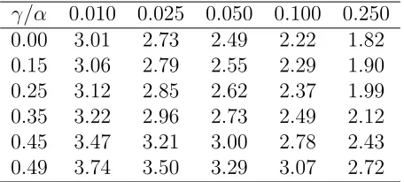
Table 2.1: Asymptotic critical values of Qτ for the open-end procedure at τ = 0.5 with p= 2.

γ/α 0.010 0.025 0.050 0.100 0.250 0.00 3.01 2.73 2.49 2.22 1.82 0.15 3.06 2.79 2.55 2.29 1.90 0.25 3.12 2.85 2.62 2.37 1.99 0.35 3.22 2.96 2.73 2.49 2.12 0.45 3.47 3.21 3.00 2.78 2.43 0.49 3.74 3.50 3.29 3.07 2.72

2.3 Simulation Study

To assess the finite sample performance of the proposed method, we conduct a simulation study. Under the null hypothesis of no sequential change point, the data were generated from the model

yi = 1 +xi+ (1 +rxi)ei, i= 1, . . . , m+Tm, (2.10) where m represents the sample size of the historical data, Tm represents the observation horizon, and r controls the heteroscedasticity of the model. The value of r = 0 gives a homoscedastic model, while r 6= 0 gives a heteroscedastic model. The processes are monitored from timem+1 until timem+Tm for several values ofTm = 2m,4m,10m,20m and 50m. We choose three cases with different choices of r and error distributions as follows:

Case 1: r= 0 (homoscedastic), ei ∼ N(0,1), xi ∼ N(0,1); Case 2: r= 0 (homoscedastic), ei ∼t2,xi ∼ N(0,1);

Case 3: r= 0.2 (heteroscedastic), ei ∼ N(0,1), xi ∼N(0,1) truncated at ±3. Case 4: r= 0 (homoscedastic), ei ∼t2,xi ∼ Unif(0,2).

We focus on two quantile levels τ = 0.5 and τ = 0.75. Besides the proposed quantile testing procedure, we also include the mean regression sequential change point detection methods in Horv´ath et al. (2004) and Xia et al. (2009). For each scenario, the simulation is repeated 3,000 times.

For power analysis, we generate data from the alternative model

yi = (

1 +xi+ (1 +rxi)ei, i= 1, . . . , m+k∗−1 1 + (1 +δ)xi+ (1 +rxi)ei, i=m+k∗, . . . , m+Tm,

(26)

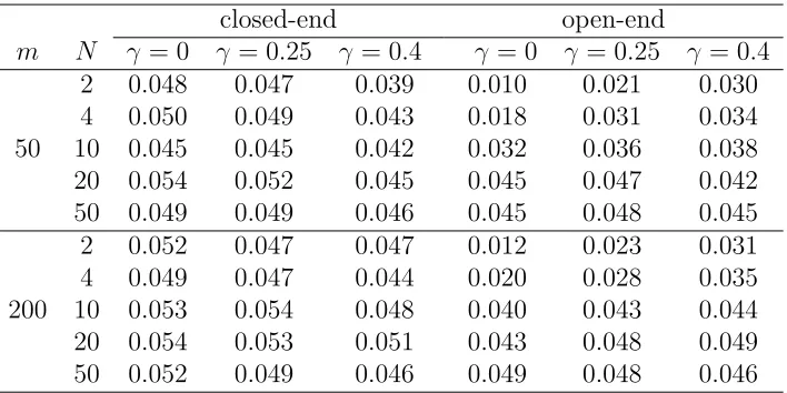
Table 2.2: Type I errors of the proposed closed- and open-end median procedures in Case 1 with γ = 0,0.25 and 0.4. The nominal significance level is 0.05.

closed-end open-end

m N γ = 0 γ = 0.25 γ = 0.4 γ = 0 γ = 0.25 γ = 0.4

50

2 0.048 0.047 0.039 0.010 0.021 0.030

4 0.050 0.049 0.043 0.018 0.031 0.034

10 0.045 0.045 0.042 0.032 0.036 0.038

20 0.054 0.052 0.045 0.045 0.047 0.042

50 0.049 0.049 0.046 0.045 0.048 0.045

200

2 0.052 0.047 0.047 0.012 0.023 0.031

4 0.049 0.047 0.044 0.020 0.028 0.035

10 0.053 0.054 0.048 0.040 0.043 0.044

20 0.054 0.053 0.051 0.043 0.048 0.049

50 0.052 0.049 0.046 0.049 0.048 0.046

where δ6= 0 represents the change in the slope.

To evaluate the performance of different methods, we consider three metrics that are commonly used in sequential change point detection. The first metric is Type I error rate, defined as the proportion of rejections for monitoring a process until timeTm under the null hypothesis associated with significance level α. The second metric is power, defined as the proportion of rejections for monitoring the process until time Tm under the alternative hypothesis. The third metric is the detection time under the alternative hypothesis.

2.3.1 Choice of

γ

Before presenting the comparative analysis results, we first assess the impact of different choices ofγ on the detecting procedure. Recall that the tuning parameterγ controls how soon the monitoring will be stopped.

(27)

closed-end procedure for N <20. For large N ≥ 20, closed- and open-end procedures perform similarly.

In addition, Table 2.2 shows that for all three γ, the Type I errors are close to their nominal levels for closed-end procedure.

Figure 2.1 plots the power curves of the proposed median regression method at three values of γ against the observation horizon Tm. The difference of the slopes in the null and alternative models is δ = 2. Here we let m = 50. Since Tm < 20m, the closed-end procedure is considered. Figure 2.1 shows that the method with γ = 0.4 has the lowest power, while the method with γ = 0 gives the highest power.

0 20 40 60 80 100

0.0 0.2 0.4 0.6 0.8 1.0

(a) Case 1, k*=10

Tm

po

w

er

γ =0

γ =0.25

γ =0.4

0 20 40 60 80 100

0.0 0.2 0.4 0.6 0.8 1.0

(b) Case 3, k*=10

Tm

po

w

er

γ =0

γ =0.25

γ =0.4

0 20 40 60 80 100

0.0

0.2

0.4

0.6

0.8

(c) Case 2, k*=10

Tm

po

w

er

γ =0

γ =0.25

γ =0.4

0 20 40 60 80 100

0.0 0.2 0.4 0.6 0.8 1.0

(d) Case 4, k*=10

Tm

po

w

er

γ =0

γ =0.25

γ =0.4

(28)

Table 2.3: Summary statistics of the distribution of detection time for different values of γ = 0,0.25 and 0.4 for the proposed closed-end procedure at median in Case 1 with Tm = 100 and δ = 2. The k∗ represents the true change point time.

m= 25, k∗ = 1

Min Q1 Median Q3 Max

γ = 0 8 27 38 54 100

γ = 0.25 3 22 35 51 100

γ = 0.4 1 20 34 55 100

m= 50, k∗ = 5

γ = 0 13 34 42 51 100

γ = 0.25 8 29 38 49 99

γ = 0.4 1 28 39 52 100

m = 100, k∗ = 1

γ = 0 14 29 34 40 74

γ = 0.25 8 22 28 35 75

γ = 0.4 4 19 26 33 80

m= 100, k∗ = 90

γ = 0 22 62 80 94 100

γ = 0.25 13 44.75 62.50 90.25 100

γ = 0.4 4 26 48.5 72 100

(29)

0 20 40 60 80 100

0.000

0.005

0.010

0.015

0.020

(a) m=25, k*=1

Detection Time

density

γ =0

γ =0.25

γ =0.4

20 40 60 80 100

0.000

0.005

0.010

0.015

0.020

0.025

0.030

(b) m=50, k*=5

Detection Time

density

γ =0

γ =0.25

γ =0.4

10 20 30 40 50 60 70 80

0.00

0.01

0.02

0.03

0.04

0.05

(c) m=100, k*=1

Detection Time

density

γ =0

γ =0.25

γ =0.4

0 20 40 60 80 100 120

0.000

0.005

0.010

0.015

0.020

(d) m=100, k*=90

Detection Time

density

γ =0

γ =0.25

γ =0.4

(30)

0.0 0.1 0.2 0.3 0.4

104

106

108

110

112

Case 1, m=200, N=2, k*=50

γ

Median Detection Time

Figure 2.3: The median detection time againstγ for the closed-end procedure at median in Case 1 with m= 200, Tm = 2m, k∗ = 50 and δ= 2.

2.3.2 Type I Error Rate

We now compare the proposed quantile regression method with the mean regression methods developed in Horv´ath et al. (2004), referred to as HHKS, and in Xia et al. (2009), referred to as XGZ. In this subsection, we let γ = 0.25 for both the quantile regression and HHKS methods.

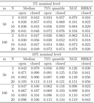
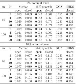
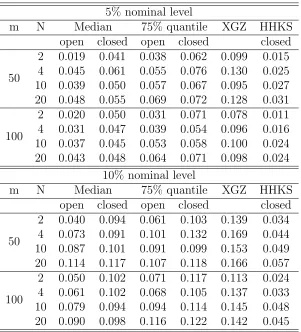
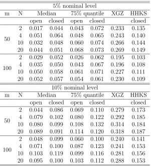
Tables 2.4-2.7 summarize the Type I errors of the proposed quantile regression method at quantile levels τ = 0.5 and 0.75, and the mean methods HHKS and XGZ in Cases 1-4, respectively. For the proposed quantile regression method, we report Type I errors for both the closed- and open-end procedures. From these tables, we can see that the XGZ method gives significantly inflated Type I errors in all scenarios except in Case 1 with m= 100. The HHKS method gives deflated Type I errors in Cases 1 and 3, and inflated Type I errors in Cases 2 and 4. Generally speaking, the proposed median method controls Type I errors better than the other two mean regression methods, especially for Cases 2 and 4 with heavy-tailed error distributions and Case 3 with heteroscedastic errors. As m increases, all the methods yield Type I errors closer to the nominal levels.

(31)

Table 2.4: Type I errors (the proportions of rejections under H0) of different methods in Case 1 with γ = 0.25. The 95% CIs for Type I errors of level-5% and level-10% valid tests are [0.0422,0.0578] and [0.0893,0.1107], respectively.

5% nominal level

m N Median 75% quantile XGZ HHKS

open closed open closed closed

50

2 0.019 0.042 0.034 0.057 0.078 0.016 4 0.038 0.057 0.052 0.069 0.101 0.022 10 0.036 0.043 0.056 0.059 0.084 0.029 20 0.041 0.046 0.072 0.076 0.104 0.031

100

2 0.014 0.047 0.030 0.063 0.062 0.014 4 0.030 0.056 0.038 0.052 0.073 0.018 10 0.041 0.047 0.054 0.061 0.073 0.023 20 0.044 0.049 0.072 0.074 0.078 0.020

10% nominal level

50

2 0.042 0.079 0.056 0.092 0.126 0.030 4 0.071 0.090 0.091 0.125 0.150 0.041 10 0.082 0.096 0.087 0.100 0.149 0.056 20 0.105 0.113 0.113 0.121 0.151 0.056

100

(32)

5% nominal level

50

2 0.013 0.039 0.042 0.067 0.193 0.094 4 0.038 0.058 0.053 0.069 0.232 0.116 10 0.039 0.050 0.066 0.074 0.231 0.122 20 0.045 0.048 0.072 0.077 0.237 0.135

100

2 0.019 0.045 0.034 0.060 0.192 0.088 4 0.031 0.055 0.038 0.060 0.215 0.101 10 0.036 0.040 0.068 0.075 0.209 0.113 20 0.044 0.048 0.057 0.063 0.225 0.115

10% nominal level

50

2 0.038 0.097 0.066 0.117 0.233 0.117 4 0.072 0.103 0.090 0.116 0.276 0.153 10 0.077 0.092 0.108 0.119 0.271 0.164 20 0.077 0.089 0.122 0.131 0.289 0.173

100

(33)

5% nominal level

50

2 0.019 0.041 0.038 0.062 0.099 0.015 4 0.045 0.061 0.055 0.076 0.130 0.025 10 0.039 0.050 0.057 0.067 0.095 0.027 20 0.048 0.055 0.069 0.072 0.128 0.031

100

2 0.020 0.050 0.031 0.071 0.078 0.011 4 0.031 0.047 0.039 0.054 0.096 0.016 10 0.037 0.045 0.053 0.058 0.100 0.024 20 0.043 0.048 0.064 0.071 0.098 0.024

10% nominal level

50

2 0.040 0.094 0.061 0.103 0.139 0.034 4 0.073 0.091 0.101 0.132 0.169 0.044 10 0.087 0.101 0.091 0.099 0.153 0.049 20 0.114 0.117 0.107 0.118 0.166 0.057

100

(34)

5% nominal level

50

2 0.017 0.044 0.043 0.072 0.233 0.135 4 0.051 0.064 0.048 0.065 0.243 0.140 10 0.032 0.048 0.060 0.074 0.266 0.144 20 0.044 0.051 0.068 0.073 0.269 0.149

100

2 0.029 0.052 0.026 0.062 0.195 0.103 4 0.035 0.050 0.043 0.067 0.196 0.108 10 0.050 0.058 0.061 0.071 0.227 0.111 20 0.052 0.057 0.054 0.061 0.230 0.109

10% nominal level

50

2 0.044 0.086 0.069 0.110 0.279 0.173 4 0.079 0.102 0.080 0.122 0.292 0.185 10 0.080 0.099 0.108 0.132 0.314 0.184 20 0.089 0.091 0.114 0.120 0.318 0.187

100

(35)

Compared to the median, the quantile method atτ = 0.75 gives Type I errors slightly larger than the nominal level, and this is possibly due to the less available information at the upper tail than at the median.

2.3.3 Power Analysis

0 100 200 300 400 500

0.0 0.2 0.4 0.6 0.8 1.0

(a) Case 1, m=50, k*=50

Tm

po

w

er

τ =0.5

τ =0.75 XGZ HHKS

0 100 200 300 400 500

0.0 0.2 0.4 0.6 0.8 1.0

(b) Case 3, m=50, k*=50

Tm

po

w

er

τ =0.5

τ =0.75 XGZ HHKS

0 100 200 300 400 500

0.0 0.2 0.4 0.6 0.8 1.0

(c) Case 2, m=50, k*=50

Tm

po

w

er

τ =0.5

τ =0.75 XGZ HHKS

0 100 200 300 400 500

0.0 0.2 0.4 0.6 0.8 1.0

(d) Case 4, m=50, k*=50

Tm

po

w

er

τ =0.5

τ =0.75 XGZ HHKS

Figure 2.4: The power curves of different methods against the observation horizon Tm in Cases 1-4, where m = 50 and δ = 2. The horizontal line represents the 5% nominal level.

(36)

generated from the alternative model (2.3.2). Figure 2.4 plots the power curves of three methods against the observation horizon Tm in Cases 1-4 with m= 50 andk∗ = 50. The difference of the pre-change and post-change slopes is δ = 2. The nominal level is 5%. Figure 2.4 suggests that as the observation horizon Tm increases, the power of all three methods increase gradually. The XGZ method appears to be the most powerful in Cases 1 and 3 but note that this higher power is associated with clearly inflated Type I errors. The HHKS method is too conservative and its power rises slowly asTmincreases in Cases 1-3, even in Case 2 where HHKS gives inflated Type I errors (see Table 2.5). In Case 4, the HHKS method is significantly improved with the uniform covariate design compared to Case 2.

Figure 2.5 plots the power curves of different methods against the slope change δ in Cases 1-4 with m = 50, N = 10,k∗ = 50. As observed in Figure 2.4, HHKS is overall too conservative in Cases 1-3. The XGZ method gives higher power at the beginning due to the large Type I errors. However, when errors have heavy tails (Cases 2 and 4), the median method catches up as δ increases, and it gives even higher power than XGZ despite its lower Type I errors when δ ≥ 0.6 for k∗ = 50 and δ ≥ 1 for k∗ = 100. The power curves of quantile method at τ = 0.75 and τ = 0.5 are similar except for Case 2, k∗ = 100, in which the power curve ofτ = 0.75 is slightly lower than at median, which is also possibly due to the less information at the upper tail than at the median. In Case 4, the HHKS method is also improved with a uniform covariate design compared to Case 2.

2.3.4 Remark

In Figures 2.4 and 2.5, we observe that the power of HHKS method increases in a much slower rate compared to other methods, especially in Case 2. To investigate this issue, we consider a modified HHKS method, which is based on the following test statistic

1 ˆ

σ1≤supk≤Tm

Pm+k

i=m+1(yi−x T iβˆ)xi g(m, k, γ)

_∞

,

whereg(m, k, γ) =m1/2(1 +k/m){k/(m+k)}γ_{, ˆ}_β_{is the LSE of}_β_{based on the historical} data set{(yi,xi), i= 1, . . . , m}.

(37)

0 2 4 6 8 10

0.0

0.2

0.4

0.6

0.8

1.0

(a) Case 1, m=50, N=10, k*=50

δ

po

w

er

τ =0.5

τ =0.75 XGZ HHKS

0 2 4 6 8 10

0.0

0.2

0.4

0.6

0.8

1.0

(b) Case 3, m=50, N=10, k*=50

δ

po

w

er

τ =0.5

τ =0.75 XGZ HHKS

0 2 4 6 8 10

0.2

0.4

0.6

0.8

1.0

(c) Case 2, m=50, N=10, k*=50

δ

po

w

er

τ =0.5

τ =0.75 XGZ HHKS

0 2 4 6 8 10

0.2

0.4

0.6

0.8

1.0

(d) Case 4, m=50, N=10, k*=50

δ

po

w

er

τ =0.5

τ =0.75 XGZ HHKS

(38)

that the Type I error is exactly 5%.

Figures 2.6 and 2.7 plot the power of different methods including the modified HHKS test against Tm (with δ = 2) and δ (with m = 50 and Tm = 500), respectively, in Cases 2 and 4. Results show that the original and modified HHKS tests have similar power in Case 4, but the modified test has clearly higher power than the original test in Case 2. Therefore, the lackness of power of the HHKS method in Case 2 is likely due to the fact that the test statistic is based on the cumulative sum of estimated residual only, while some power improvement can be achieved by incorporating the covariate in the score function involved in the test statistic.

0 100 200 300 400 500

0.0

0.2

0.4

0.6

0.8

1.0

(a) Case 2, normal covariate

Tm

po

w

er

τ =0.5 XGZ HHKS modi HHKS

0 100 200 300 400 500

0.0

0.2

0.4

0.6

0.8

1.0

(b) Case 2, uniform covariate

Tm

po

w

er

(39)

0 2 4 6 8 10

0.0

0.2

0.4

0.6

0.8

1.0

(a) Case 2, normal covariate

δ

po

w

er

0 2 4 6 8 10

0.0

0.2

0.4

0.6

0.8

1.0

(b) Case 2, uniform covariate

δ

po

w

er

(40)

2.4 Monitoring Change Points Across Quantiles

2.4.1 Hypotheses and the Proposed Method

Suppose we are studying the relationship of salary and gender of employees in an industry. If we are interested in monitoring whether the impact of gender has any change on the distribution of salary over time, especially at the lower tails of the salary distribution, then the interested quantile levels can be pre-specified as a range such as (0,0.1]. By looking at multiple quantiles, we can obtain a more complete picture of the conditional distribution than only looking at a single quantile. Therefore, it is desirable to carry out the test across quantiles to monitor the structural changes.

Let T be a closed set of (0,1) containing the quantiles of interest. In the subsequent analysis, we assumeT = [ω,1−ω] for some 0< ω <1/2. We assume the following linear quantile regression model

Qyi(τ|xi) =x

T

i βi,τ, for all τ ∈ T, i≥1.

The proposed test across quantiles is also based on the “noncontamination” assumption as introduced in Section 2.2, that is, β₁_,τ = . . . = β_m,τ = β₀_,τ. We are interested in testing the null hypothesis

H₀∗ :β_i,τ =β₀_,τ, for all τ ∈ T, and i≥m+ 1, (2.12)

against the alternative hypothesis

H₁∗ :β_i,τ = (

β₀_,τ, for m+ 1≤i < m+k∗

β₁_,τ, for i≥m+k∗, (2.13)

where k∗ ≥1 is the unknown change point, and β₀_,τ 6=β₁_,τ for someτ ∈ T.

Extending the idea of change point monitoring for a single quantile level in Section 2.2, we propose the following test statistic

M QT = sup

τ∈T

sup 1≤k≤Tm

D_m−1/2 m+k X i=m+1

xiψτ(yi−xTi βˆτ) g(m, k, γ)

∞

, (2.14)

(41)

k/m){k/(m+k)}γ_,_D

m =m−1Pm_i₌₁xixTi , and ψτ(u) = τ−I(u <0).

2.4.2 Asymptotic Properties

In this subsection, we will establish the asymptotic properties of the proposed statistic M QT.

Theorem 3 Suppose that assumptions A1-A3 hold.

(i) For the open-end procedure withTm → ∞ and the closed-end procedure with Tm/m→ ∞ as m→ ∞, under the null hypothesis H₀∗, we have

M QT D

−→sup τ∈T

sup 0≤t≤1

kW(t, τ)k∞

tγ ,asm→ ∞; (2.15)

(ii) For the closed-end procedure with Tm < ∞ and limm→∞Tm/m = N for some 0 < N <∞, under the null hypothesis H₀∗, we have

M QT D

−→sup τ∈T

sup 0≤t≤N/(N+1)

kW(t, τ)k∞

tγ ,as m→ ∞, (2.16)

where W(t, τ) = {W1(t, τ), . . . , Wp(t, τ)} denotes a p-dimensional independent two-parameter Gaussian process with mean 0, and covariance

E{Wj(t, τ), Wj(t0, τ0)}= min(t, t0){min(τ, τ0)−τ τ0}, (2.17)

where j = 1, . . . , p.

Based on the asymptotic results of Theorem 3(i), we can calculate the critical values of M QT when Tm =∞ orTm/m→ ∞ through simulation using the following steps.

1. Let 0< τ1 < . . . < τnτ be a sequence of quantile levels from T.

2. Generate a sequence of i.i.d.p-dimensional random vector ei = (ei1, . . . , eip), where eij

i.i.d.

∼ Unif(0,1), i= 1, . . . , M, with M = 10,000. 3. Define W_j∗(t, τ) = M−1/2P[tM]

i=1 {I(eij ≤τ)−τ}, j = 1, . . . , p and t∈ T1 ={1/M,2/M, . . . ,1}. Calculate the statistic

M Q1 = sup 1≤s≤nτ

sup t∈T1

(42)

where W∗(t, τ) = {W∗

1(t, τ), . . . , W

∗

p(t, τ)}.

4. By repeating Steps 1-3 for B = 50,000 times, we can get M Q1, . . . , M QB. The critical value for a level-αtest based onM QT can then be estimated by the (1−τ)th

quantile of M Q1, . . . , M QB.

Based on the asymptotic results of Theorem 3(ii), we can calculate the critical values ofM QT whenTm <∞ andTm/m→N for some 0< N <∞through simulation by the following steps.

1. Let 0< τ1 < . . . < τnτ be a sequence of quantile levels from T.

2. Generate a sequence of i.i.d.p-dimensional random vector ei = (ei1, . . . , eip), where eij

i.i.d.

∼ Unif(0,1), i= 1, . . . , M, with M = 10,000. 3. Define W_j∗(t, τ) = M−1/2P[tM]

i=1 {I(eij ≤τ)−τ}, j = 1, . . . , p and t∈ T2 = {1/M,2/M, . . . , N/(N + 1)}. Calculate the statistic

M Q∗₁ = sup 1≤s≤nτ

sup t∈T2

kW∗(t, τs)k∞t−γ,

where W∗(t, τ) = {W∗

1(t, τ), . . . , Wp∗(t, τ)}.

4. By repeating Steps 1-3 for B = 50,000 times, we can get M Q∗₁, . . . , M Q∗_B. The critical value for a level-αtest based onM QT can then be estimated by the (1−τ)th

quantile of M Q∗₁, . . . , M Q∗_B.

Table 2.8 provides the asymptotic critical values of the proposed method under both the closed- and the open-end procedures across quantilesτ ∈ T ={ω, ω+ 0.1, . . . ,1−ω} for some ω >0.

Remark 2 Below we provide some justification for the proposed critical value calculation procedure. DenoteW∗(t, τ) =M−1/2PtM

i=1{I(ei ≤τ)−τ}, whereei = (ei1, . . . , eip), where eij

i.i.d.

∼ Unif(0,1), i = 1, . . . , M, j = 1, . . . , p. Then by the CLT, as M → ∞, W_j∗(t, τ) converges to a Gaussian process with mean E{W∗

j(t, τ)} = E[M−1/2 PtM

(43)

Table 2.8: Asymptotic critical values of the statistic MQ across τ ∈[ω,1−ω] with the number of regressors p = 2 for γ=0, 0.25 and 0.4, and nominal level α = 0.05 and 0.1. The results are based on 50,000 Monte Carlo replications.

γ ω closed open

α = 0.05 α = 0.1 α= 0.05 α= 0.1 0

0.10 1.1404 1.0375 1.3953 1.2790 0.15 1.1382 1.0398 1.3975 1.2768 0.20 1.1404 1.0375 1.3953 1.2790 0.25

0.10 1.3099 1.2055 1.4519 1.3373 0.15 1.3096 1.2063 1.4519 1.3390 0.20 1.3099 1.2054 1.4519 1.3373 0.4

0.10 1.4760 1.3728 1.5457 1.4317 0.15 1.4758 1.3747 1.5425 1.4329 0.20 1.4760 1.3724 1.5457 1.4317

τ}] = 0, and covariance

E{W∗

j(t, τ)W

∗

j(t

0_{, τ}0_)}

=E "

M−1/2 tM X

i=1

{I(ei ≤τ)−τ}M−1/2 t0M X

k=1

{I(ek ≤τ0)−τ0} #

=M−1E (_tM

X i=1

I(ei ≤τ) t0M X k=1

I(ek ≤τ0) )

−t0τ0E (_tM

X i=1

I(ei ≤τ) )

−tτ E (_t0_M

X k=1

I(ek ≤τ0) )

+M tτ t0τ0

=(M tt0−t∧t0)τ τ0+ (t∧t0)(τ∧τ0)−M tt0τ τ0 =(t∧t0)(τ∧τ0−τ τ0),

which agrees with the covariance in (2.17). Here a∧b≡min(a, b).

2.4.3 Simulation Study

(44)

The processes are monitored from time m+ 1 until time m +Tm for several values of Tm = 2m,10m,20m, andm = 50 or 200. We consider T ={0.1,0.2, . . . ,0.9}.

Table 2.9 summarizes the Type I errors of the proposed multi-quantile method for both the closed- and open-end procedures in Cases 1-4. In general, the closed-end procedure gives slightly inflated Type I errors, and the open-end procedure tends to give deflated Type I errors. In addition, the effect of N on the open-end procedure is more obvious than that on the closed-end procedure. As N increases, the Type I errors for the open-end procedure topen-end to increase and become close to the nominal levels in all cases. In contrast, the Type I errors for the closed-end procedure are stable acrossN. In addition, asmincreases, the Type I errors of both procedures are reduced, which leads to different effects on two procedures: the closed-end procedure gives Type I errors close to the nominal levels, while the open-end procedure tends to be more conservative in all three studied cases, especially for smaller values of N, for instance N = 2 and 4.

(45)

Table 2.9: Type I errors (the proportions of rejections under H0) of the proposed multiple-quantile method and median method in Cases 1-4 with γ = 0.25. The 95% CIs for Type I errors of level-5% and level-10% valid tests are [0.0422,0.0578] and [0.0893,0.1107], respectively.

Case 1

α m N = 2 N = 10

closed open median closed open median 5% 50 0.0700 0.0350 0.0470 0.0780 0.0527 0.0440

200 0.0583 0.0197 0.0467 0.0660 0.0400 0.0660 10% 50 0.1200 0.0610 0.0933 0.1393 0.0973 0.0953 200 0.1133 0.0500 0.0923 0.1250 0.0830 0.1127

Case 2

α m N = 2 N = 10

200 0.0493 0.0193 0.0457 0.0740 0.0483 0.0677 10% 50 0.1257 0.0623 0.0897 0.1340 0.1140 0.0943 200 0.1083 0.0437 0.0880 0.1417 0.0900 0.1203

Case 3

α m N = 2 N = 10

200 0.0600 0.0233 0.0493 0.0573 0.0467 0.0623 10% 50 0.1207 0.0617 0.1003 0.1273 0.1103 0.1010 200 0.1130 0.0497 0.0950 0.1140 0.0950 0.1123

Case 4

α m N = 2 N = 10

(46)

0.5 1.0 1.5 2.0

0.2

0.4

0.6

0.8

1.0

(a) Case 1, m=200, N=2, k*=100

δ

po

w

er

multi median q1 q3

0.5 1.0 1.5 2.0

0.2

0.4

0.6

0.8

1.0

(b) Case 2, m=200, N=2, k*=100

δ

po

w

er

multi median q1 q3

0.5 1.0 1.5 2.0

0.2

0.4

0.6

0.8

1.0

(c) Case 3, m=200, N=2, k*=100

δ

po

w

er

multi median q1 q3

0.5 1.0 1.5 2.0

0.2

0.4

0.6

0.8

1.0

(d) Case 4, m=200, N=2, k*=100

δ

po

w

er

multi median q1 q3

(47)

2.5 Analysis of a S&P 500 Index Data Set

We apply the proposed testing procedure to analyze a S&P 500 index dataset. The dataset contains the monthly returns of S&P 500 index from February 1988 to November 2012 with total 298 observations. We consider the response variable yi as the monthly total returns of S&P 500 index, and the explanatory variablexi as the previous month’s earnings to price (EP) ratio. The EP ratio is defined as annual earnings per share divided by market price per share. We aim to monitor the stability of the effect of monthly EP ratio on monthly total return of S&P 500 index as time goes by. The data can be downloaded from http://www.multpl.com/table?f=mandhttp://research.

stlouisfed.org/fred2/series/SP500/downloaddata?cid=32255.

We set the first m = 50 observations (from February 1988 to March 1992) as the history

data, for which the regression coefficients were shown to be stable based on the testing method

of Qu (2008) at the median. The mean regression methods HHKS in Huskova and Kirch (2012)

and XGZ in Xia et al. (2009) fail to detect any change in the linear regression coefficients.

The proposed median regression method detects four change points with the estimated

quantile functions as

Qy(τ = 0.5|xi) =           

         

−0.0075 + 0.3623xi, 1≤i≤67

−0.0108 + 0.5691xi, 68≤i≤123

−0.0659 + 2.1509xi, 124≤i≤190

0.0003 + 0.2161xi, 191≤i≤257

0.0403−0.4239xi, 258≤i≤298.

The four change points correspond to 09/1993, 05/1998, 12/2003 and 07/2009, respectively. The

estimations in the five segments show that the total return was positively related to EP ratio

before 1993, but the slope increased slightly until the change point was detected in 05/1998, a

year after the dot-com bubble began. After 05/1998, the slope continued to increase at a larger

degree to 2.1509 and it then dropped to 0.2161 starting from 12/2003, around the time that

the dot-com bubble ended. Since then the slope continued to drop to negative after 07/2009,

shortly after financial crisis of 2008.

Besides median, we also apply the proposed method to the quantile τ = 0.75. The analysis

(48)

and around the end of the dot-com bubble. The estimated quantile functions are

Qy(τ = 0.75|xi) =     

   

0.0407−0.0021xi, 1≤i≤132

−3.84 + 0.43xi, 133≤i≤198

7.64−0.04xi, 199≤i≤298.

The estimations show that the slope increased after the burst of dot-com bubble, and it

(49)

2.6 Proof

Throughout the proof, we let Ci, i = 1, . . . ,7 denote some positive constants. Before proving

Theorem 1, we present the following two lemmas.

Lemma 1 Let C1 be some positive constants. Define S = {(˜t, τ) : k˜tk ≤ C1, τ ∈ T } and

rm,k(˜t, τ) = Pmi=+mk+1xi

ψτ(yi−xTi β0τ−m−1/2xTi˜t)−ψτ(yi−xTiβ0τ) . Then there exist some positive constants C2 andC3 such that for sufficiently large m and k,

P

(

sup

S

krm,k(˜t, τ)−E{rm,k(˜t, τ)|x}k ≥C2λmax(m−1/4k1/2, k1/4) p

logk

)

≤C3k−λ.

Proof.For fixed ˜t such thatk˜tk< C1 and τ ∈(0,1), define

Ri=xi{ψτ(yi−xTiβ0τ−m

−1/2_xT

i˜t)−ψτ(yi−xTi β0τ)}

=

(

−xisgn(xTi˜t), ifyi∈Ji

0, otherwise,

where Ji represents the interval between xTi β0τ and xTi β0τ +m−1/2xTi˜t, and sgn(·) represents

the sign function. For thejth coordinate ofRi,Rij,j = 1, . . . , p, we have

=x2_ijfy(u|xi)m−1/2|xTi ˜t|< C4x2ijpmax|xij|m−1/2,

where u is some value between xT_i β0_τ and xT_i β0_τ +m−1/2xT_i ˜t. By assumptions A2 and A3 (ii),

we have Pm_m+₊₁kVar(Rij|xi) ≤C4m−1/2Pm_m+₊₁kkxik4 and k−1Pm_m₊₁+kkxik4 ≤ B for some finite

constantB. Thus, Pm+k

m+1Var(Rij|xi)≤C5m

−1/2_k._{In addition, by assumption A3 (i), we have}

maxm+1≤i≤m+kkRik ≤maxm+1≤i≤m+kkxik=Op(k1/4/

√

logk).

Letδm,k = max{C5k/

√ m, C2

6(2/log 2)2

√

k}. By the Hoeffding inequality, there exists a constant

C7 such that for sufficiently large λandk, we have

P{kr_m,k−E(rm,k|x)k ≥(1 +λ) p

δm,k p

logk}

=P{kr_m,k−E(rm,k|x)k ≥C7λmax(k1/2m−1/4, k1/4)

p

logk}

≤2 exp(−λlogk) = 2k−λ.

The rest of the proof for the uniform convergence can be obtained by following a chaining

argument similar to that used in the proof of Lemma A.2 in Koenker and Portnoy (1987) and

(50)

Lemma 2 Define Rm,k = max(m−1/4k1/2, k1/4)

√

logk+ (k/m)1/4. Then for γ ∈(0,1/2) and

ν >2, we have

k1/ν+km1/ν−1+km−1/2o(1) +O(Rm,k)

m1/2_{(1 +}_k/m₎_{_k/₍_m₊_k₎_}γ →0, asm→ ∞. (2.18)

Proof.Note that

k1/ν+km1/ν−1+km−1/2o(1) +O(Rm,k)

m1/2_{(1 +}_k/m₎_{_k/₍_m₊_k₎_}γ

= k

1/ν

m1/2_{(1 +}_k/m₎_{_k/₍_m₊_k₎_}γ +

k/m

(1 +k/m){k/(m+k)}γm

1/ν−1/2

+ k/m

(1 +k/m){k/(m+k)}γo(1) +

O(Rm,k)

m1/2_{(1 +}_k/m₎_{_k/₍_m₊_k₎_}γ

.

=A1+A2+A3+A4. (2.19)

We consider two cases separately.

Case 1:1≤k≤m. As m→ ∞, it is easy to show that

A2 =

k

(m+k){k/(m+k)}γm

1/ν−1/2 ₌_{_k/₍_m₊_k₎_}1−γ_m1/ν−1/2₌_o₍₁₎_,

A3 =

k

(m+k){k/(m+k)}γo(1) ={k/(m+k)}

1−γ_o_{(1) =}_o₍₁₎ _and

A1 =

k1/ν−γ

m1/2_{(1 +}_k/m₎₍_m₊_k₎−γ <

k1/ν−γ m1/2₍₂_m₎−γ =

2γk1/ν−γ

m−γ+1/2.

If 1/ν≥γ,A1 ≤2γm1/ν−γ+γ−1/2 →0,otherwise

A1 =

k1/ν−γ

m1/2_m−1₍_m₊_k₎₍_m₊_k₎−γ =

m1/2

(m+k)1−γ_kγ−1/ν

< m

1/2

(m+k)1−γ <

m1/2 m1−γ =m

(51)

In addition,

A4=

{max(m−1/4k1/2, k1/4)√logk+ (k/m)1/4}O(1) m1/2_{(1 +}_k/m₎_{_k/₍_m₊_k₎_}γ

=

"

m1/2−1/4

(m+k)3/4

k1/4−γ

(m+k)1/4−γ + max

(

m−1/4 m−1/2₍_m₊_k₎1/4

k3/4−γ

(m+k)3/4−γk

−1/4p

logk,

1

m−1/2₍_m₊_k₎1/2

k1/2−γ

(m+k)1/2−γk

−1/4p

logk )# O(1) = " k

m+k

1/4−γ

m1/4

(m+k)3/4 + max

(

m

m+k

1/4

k

m+k

3/4−γ

k−1/4plogk,

m

m+k

1/2

k

m+k

1/2−γ

k−1/4plogk

)#

O(1). (2.20)

Since γ ∈(0,1/2) and k−1/2/√logk→0, it is easy to show that (2.20)→0.

Case 2:m≤k≤ ∞. Asm→ ∞, we can show that

A1 =

k1/ν−γm1/2

(m+k)1−γ ≤

k1/ν−γm1/2

k1−γ =k

1/ν−1_m1/2 _→₀_,

A2 =

k

m+k

1−γ

m1/ν−1/2=o(1) and

A3 =

k/m

(1 +k/m){k/(m+k)}γo(1) =o(1).

In addition,

A4 ≤max

(

m

m+k

1/4

k

m+k

3/4−γ

,

m

m+k

1/2

k

m+k

1/2−γ)

k−1/4plogk

+

k

m+k

1/4−γ

m1/4

(m+k)3/4 < k

−1/4p

(52)

Proof of Theorem 1. Let ˜t be ap-dimensional vector that is bounded. By applying Lemma

1 to a prespecified quantile levelτ, we have

m+k X

i=m+1

xiψτ(yi−xTi βτ0−m−1/2xTi ˜t)− m+k

X

i=m+1

xiψτ(yi−xTi β0τ)

=E

( _m₊_k

X

i=m+1

xiψτ(yi−xTi βτ0−m−1/2xTi˜t)− m+k

X

i=m+1

xiψτ(yi−xTi β0τ) xi

)

+Op(Rm,k)

=

m+k X

i=m+1

xi{τ−P(yi ≤xTi β0τ +m−1/2xi˜t|xi)} − m+k

X

i=m+1

xi{τ −P(yi ≤xTi β0τ|xi)}+Op(Rm,k)

=

m+k X

i=m+1

xi{Fy(xTi βτ0|xi)−Fy(xTi β0τ+m−1/2xTi t|x˜ i)}+Op(Rm,k)

=−

m+k X

i=m+1

xify(xTi β0τ|xi)m−1/2xTi˜t+Op(Rm,k) +op(R(1)_m,k)

=−

m+k X

i=m+1

xify(xTi β0τ|xi)m−1/2xTi˜t+Op(Rm,k), (2.22)

where Rm,k = max(m−1/4k1/2, k1/4)

√

logk+ (k/m)1/4, and R(1)_m,k =km−1/2.

By Koenker and Bassett (1978), m1/2_{( ˆ}_β0

τ −β0τ) = Op(1). Therefore, by plugging ˜t =

m1/2( ˆβ0_τ−β0_τ) into (2.22), we have

m+k X

i=m+1

xiψτ(yi−xTi βˆ 0 τ)−

m+k X

i=m+1

=−

m+k X

i=m+1

fy(xTiβ0τ|xi)xixTi ( ˆβ 0

τ−β0τ) +Op(Rm,k) +op(km−1/2). (2.23)

From (4.4) of Koenker (2005), we have the Bahadur representation of ˆβ0_τ as follows

m1/2( ˆβ0_τ−β0_τ) =D₁−1(τ)m−1/2

m X

i=1

xi{τ −I(yi <xTi β0τ)}+Op(m−1/4 p

(53)

Plugging (2.24) into (2.23) gives

m+k X

i=m+1

xiψτ(yi−xTi βˆ 0 τ)−

m+k X

i=m+1

=−

m+k X

i=m+1

fy(xTi β0τ|xi)xixTi m−1/2  



D−₁1(τ)m−1/2

m X

j=1

xiψτ(yj−xTjβ0τ)

+op(m−1/4

p

logm)o+Op(Rm,k) +op(km−1/2)

=−k

(

k−1

m+k X

i=m+1

fy(xTi βτ0|xi)xixTi )

D₁−1(τ)

 



m−1

m X

j=1

xjψτ(yj −xTjβ0τ)  



+km−1/2op(m−1/4

p

logm) +Op(Rm,k) +op(km−1/2)

=−k{D1(τ) +op(1)}D1−1(τ)

 



m−1

m X

j=1

xjψτ(yj−xTjβ0τ)  



+op(km−3/4

p

logm)

+Op(Rm,k) +op(km−1/2)

=−km−1

m X

j=1

xjψτ(yj−xTjβ0τ) +op(km−1/2) +Op(Rm,k). (2.25)

Therefore,

J−1/2

m+k X

i=m+1

xiψτ(yi−xTi βˆ 0 τ)

=J−1/2

m+k X

i=m+1

xiψτ(yi−xTi β0τ)−km−1J−1/2 m X

i=1

+op(km−1/2) +Op(Rm,k). (2.26)

By the FCLT approximation on page 837 of Leisch et al. (2000b), for each m, we can find

two independentp-dimensional Wiener processes{W1,m(t)} and{W2,m(t)} forν >2 such that

sup

1≤k<∞ k−1/ν

J−1/2

m+k X

i=m+1

xiψτ(yi−xTiβ0τ)−W1,m(k) ∞

=Op(1), (2.27)

and

J−1/2

m X

i=1

xiψτ(yi−xTi β0τ)−W2,m(m) ∞

Sequential Change Point Detection.

ABSTRACT

DEDICATION

BIOGRAPHY

ACKNOWLEDGEMENTS

TABLE OF CONTENTS

LIST OF TABLES

LIST OF FIGURES

Chapter 1

Introduction

1.1

Introduction to Change Point Detection

1.2

Introduction to Quantile Regression

1.3

Outline of the Dissertation

Chapter 2