ABSTRACT
YU, ZHE. Total Recall and Software Engineering. (Under the direction of Tim Menzies).
Software engineering is a discipline closely involved with human activities. How to help software developers produce better software more efficiently is the core topic of software engineering. Prioritizing tasks can efficiently reduce the human efforts and time required to retrieve certain relevant software artifacts (e.g. relevant research papers, security vulnerabilities in the code, test cases detecting faults, etc.). Many of such prioritization problems in software engineering can be generalized as the total recall problem. The total recall problem aims to optimize the cost for achieving very high recall—as close as practicable to 100%—with a human assessor in the loop. This problem has been explored in information retrieval for years, and the state of the art solution with active learning and natural language processing aims to resolve the following challenges:
• Higher recall and lower cost.Among a finite number of tasks, which task to be executed first so that most of the relevant artifacts can be retrieved earlier?
• When to stop.At what point, there is no need to execute the remaining tasks?
• Human error correction.Are all the tasks executed correctly? How to identify wrongly executed tasks and correct them?
Although being explored for years, all three challenges have much room to be improved.
We claim that a broad class of software engineering problems, where humans must apply their expert knowledge to identify target software artifacts from a tediously large space, can be generalized as the total recall problem and be better solved by active learning. To support this claim, we studied the existing state of the art techniques in solving the total recall problems, and proposed a new active learning-based framework, FASTREAD, to resolve the three challenges of total recall. FASTREAD was tested on software engineering literature review datasets and were found to outperform the existing state of the art solutions. We also conducted our own literature review study with FASTREAD. With six other graduate students validating the FASTREAD selection result, FASTREAD was shown to have reduced 50 (from 54 to 4) human-hours study selection cost without missing important relevant information. After that, we conjecture that another two software engineering problems—test case prioritization and software security vulnerability prediction—can also be generalized as the total recall problem. With little adaptation, FASTREAD was applied to solve the software security vulnerability prediction problem successfully.
© Copyright 2020 by Zhe Yu
Total Recall and Software Engineering
by Zhe Yu
A dissertation submitted to the Graduate Faculty of North Carolina State University
in partial fulfillment of the requirements for the Degree of
Doctor of Philosophy
Computer Science
Raleigh, North Carolina 2020
APPROVED BY:
Laurie Williams Christopher Parnin
Chi Min Tim Menzies
DEDICATION
BIOGRAPHY
ACKNOWLEDGEMENTS
TABLE OF CONTENTS
Chapter 1 INTRODUCTION. . . 1
1.1 Statement of Thesis . . . 2
1.2 Research Questions . . . 2
1.3 Novel Contributions of this Work . . . 2
1.4 Papers from This Dissertation . . . 3
1.4.1 Accepted Papers . . . 3
1.4.2 Papers Under Review . . . 3
1.5 Structure of this Thesis . . . 4
Chapter 2 TOTAL RECALL . . . 5
2.1 Definition . . . 5
2.2 Motivation . . . 5
2.2.1 Electronic Discovery . . . 6
2.2.2 Evidence-based Medicine . . . 6
2.2.3 Primary Study Selection . . . 7
2.2.4 Test Case Prioritization . . . 7
2.2.5 Software Security Vulnerability Prediction . . . 8
2.3 Challenges of Total Recall Problem . . . 8
2.3.1 Higher Recall and Lower Cost . . . 8
2.3.2 When to Stop . . . 11
2.3.3 Human Error Correction . . . 12
2.3.4 Scalability . . . 13
2.4 Summary . . . 13
Chapter 3 FASTREAD . . . 14
3.1 FASTREAD Operators . . . 14
3.2 FASTREAD Framework . . . 15
3.3 Summary . . . 17
Chapter 4 CASE STUDY #1: FINDING RELEVANT RESEARCH PAPERS . . . 18
4.1 Introduction . . . 18
4.2 Background . . . 21
4.2.1 Literature Reviews in Different Domains . . . 21
4.2.2 Automatic Tool Support . . . 21
4.2.3 Abstract-based Methods . . . 22
4.3 Datasets . . . 23
4.4 Higher recall and lower cost . . . 23
4.4.1 Related work . . . 24
4.4.2 Methodology . . . 24
4.4.3 Experiments . . . 27
4.4.4 Results . . . 27
4.4.5 Summary . . . 29
4.5 How to start . . . 30
4.5.1 Related Work . . . 31
4.5.3 Results . . . 33
4.5.4 Summary . . . 34
4.6 When to Stop . . . 35
4.6.1 Related Work . . . 35
4.6.2 Method . . . 35
4.6.3 Experiments . . . 36
4.6.4 Results . . . 36
4.6.5 Summary . . . 38
4.7 Human error correction . . . 38
4.7.1 Related Work . . . 40
4.7.2 Method . . . 40
4.7.3 Experiments . . . 42
4.7.4 Results . . . 43
4.7.5 Summary . . . 43
4.8 Summary . . . 44
Chapter 5 CASE STUDY #2: A REAL-WORLD LITERATURE REVIEW WITH FAS-TREAD . . . 45
5.1 Introduction . . . 45
5.2 Case Study: A Systematic Literature Review on Test Case Prioritization with FASTREAD 48 5.2.1 Phase 1—planning . . . 49
5.2.2 Phase 2—execution . . . 51
5.2.3 Phase 3—reporting . . . 53
5.3 Validation . . . 55
5.3.1 RQ1: What percentage of relevant papers did FASTREAD actually retrieve? . . . 55
5.3.2 RQ2: What information is missing in the final report because of FASTREAD? . 57 5.4 Conclusions and Future Work . . . 59
Chapter 6 CASE STUDY #3: TEST CASE PRIORITIZATION . . . 61
6.1 Introduction . . . 61
6.2 Background and Related Work . . . 64
6.2.1 Automated UI Testing . . . 64
6.2.2 Test Case Prioritization . . . 65
6.2.3 Prioritizing Automated UI Test Cases . . . 67
6.3 Methodology . . . 67
6.3.1 TERMINATOR . . . 67
6.4 Empirical Study . . . 69
6.4.1 Dataset . . . 69
6.4.2 Independent Variables . . . 69
6.4.3 Dependent Variables . . . 75
6.4.4 Threats to Validity . . . 76
6.4.5 Results . . . 76
6.5 organizational impacts . . . 78
6.6 Conclusion . . . 78
Chapter 7 CASE STUDY #4: SECURITY VULNERABILITY PREDICTION . . . 80
7.1 Introduction . . . 80
7.2 Background and Related Work . . . 82
7.2.1 Vulnerability Prediction . . . 82
7.3 HARMLESS . . . 83
7.4 HARMLESS Simulation . . . 84
7.4.1 Dataset . . . 84
7.4.2 Simulation on Mozilla Firefox Dataset . . . 86
7.5 Experiments . . . 87
7.5.1 Experiment for Vulnerability Inspection Efficiency . . . 87
7.5.2 Experiment for Stopping Rule . . . 88
7.5.3 Experiment for Human Errors . . . 88
7.6 Results . . . 90
7.7 Conclusion . . . 94
Chapter 8 CONCLUSION. . . 96
8.1 When does FASTREAD (Not) Work . . . 96
8.2 Limitations of Current Work . . . 96
8.2.1 Threats to Validity . . . 97
8.2.2 Other Limitations . . . 97
8.3 Future Work . . . 98
8.3.1 Generalizability . . . 98
8.3.2 Human Bias . . . 99
8.3.3 Cold Start . . . 99
CHAPTER
1
INTRODUCTION
Software engineering (SE) is a discipline closely involved with human activities. How to help software developers produce better software more efficiently is the core topic of software engineering. Prioritizing tasks can efficiently reduce the human efforts and time required to achieve certain goals of software development. Many of such prioritization problems in software engineering can be generalized as the total recall problem.
The total recall problem aims to optimize the cost for achieving very high recall–as close as practicable to 100%–with a human assessor in the loop. This problem has been explored in information retrieval for years, and the state of the art solution with active learning focuses on incrementally learn an active learning model to predict which task to be executed next, so that certain goals can be achieved earlier by executing fewer tasks. In this manner, the expensive human efforts can be directed to the most valuable tasks. This active learning strategy has been proven to be effective in guiding humans to retrieve relevant information via reading text. However, there is still large room to improve for the total recall solutions, especially on the following three practical questions:
• How to better avoid wasting human effort on invaluable tasks? • At what point, there is no need to execute the remaining tasks?
• Are all the tasks executed correctly? How to identify wrongly executed tasks and correct them? In this work, we first propose an improved active learning framework, called FASTREAD, with a set of novel algorithms to better solve the total recall problem. FASTREAD is developed and tested on a case study where software engineering researchers screen thousands of abstracts to find dozens of relevant studies to their research (primary study selection). On this primary study selection case study, FASTREAD outperforms the existing total recall solutions by:
• guiding the process to stop at a target recall through accurately estimating the number of relevant studies to be found;
• detecting and correcting more human errors with lower cost, by asking humans to recheck the classifi-cation results where current active learner disagree most on.
We also conducted our own literature review study with FASTREAD. With six other graduate students validating the FASTREAD selection result, FASTREAD was shown to have reduced 50 (from 54 to 4) human-hours study selection cost without missing important relevant information. In addition, we believe that, beyond the primary study selection problem, there is a broad class of software engineering problems that can be generalized as total recall problems and can be better solved with the new FASTREAD approach. To justify this point, we applied and adapted FASTREAD to two more software engineering problems:
1. test case prioritization,
2. software security vulnerability prediction.
Results show that this novel solution to total recall problem, FASTREAD, helps solve the above software engineering problems in various aspects. Therefore we claim that identifying and exploring the total recall problems in software engineering is an important task which benefits both software engineering research and the general solution to total recall problems.
1.1
Statement of Thesis
A broad class of software engineering problems, where humans must apply their expert knowledge to identify target software artifacts from a tediously large space, can be generalized as the total recall problem and be better solved by active learning.
1.2
Research Questions
We ask the following three research questions for every case study if applicable:
RQ1: “Higher recall and lower cost”. How much cost can FASTREAD save when reaching a target high recall? Does it cost less than the prior state of the art methods?
RQ2: “When to stop”. How accurate can FASTREAD estimate for the current recall? Can it stop at a user specified recall using the estimation?
RQ3: “Human error correction”. Can FASTREAD efficiently identify and fix human errors without imposing too much extra cost?
1.3
Novel Contributions of this Work
In summary, the contributions of this work are:
2. FASTREAD, a novel and effective active learning framework for solving the total recall problem. 3. A demonstration that FASTREAD achieves higher recall with lower cost than the prior state of the art
solutions for the total recall problem.
4. An estimator that can be applied along with the execution of FASTREAD to accurately estimate the current recall. This estimator can be used to provide guidance to stop the process at target recall. 5. An error correction mechanism in FASTREAD that detects human errors without imposing excessive
extra human effort.
6. A demonstration that FASTREAD can be successfully applied to solve total recall problems across domains.
7. A reproduction package of the FASTREAD framework on Zenodo [YM17] and a tool continuously updated on Github1.
1.4
Papers from This Dissertation
1.4.1 Accepted Papers
• [Yu19]Zhe Yu, Christopher Theisen, Laurie Williams, and Tim Menzies. “Improving Vulnerability Inspection Efficiency Using Active Learning”. IEEE Transactions on Software Engineering (2020). • [Yu19b]Zhe Yu, Fahmid Fahid, Tim Menzies, Gregg Rothermel, Kyle Patrick, and Snehit Cherian.
“TERMINATOR: Better Automated UI Test Case Prioritization”. In Proceedings of ESEC/FSE’19 SEIP.
• [YM19]Zhe Yu and Tim Menzies. “FAST2: An intelligent assistant for finding relevant papers”. Expert Systems with Applications 120 (2019), pp. 57-71.
• [Yu18]Zhe Yu, Nicholas A. Kraft, and Tim Menzies. “Finding better active learners for faster literature reviews”. Empirical Software Engineering (2018), pp. 1-26.
• [YM18]Zhe Yuand Tim Menzies. “Total recall, language processing, and software engineering.” In Proceedings of the 4th ACM SIGSOFT International Workshop on NLP for Software Engineering, pp. 10-13. ACM, 2018.
• [Nai18] Vivek Nair, Amritanshu Agrawal, Jianfeng Chen, Wei Fu, George Mathew, Tim Menzies, Leandro Minku, Markus Wagner, andZhe Yu. “Data-Driven Search-based Software Engineering.” In Proceedings of Mining Software Repositories (MSR) 2018.
1.4.2 Papers Under Review
• [Yu19a]Zhe Yu, Jeffrey C Carver, Gregg Rothermel, and Tim Menzies. “Searching for Better Test Case Prioritization Schemes: a Case Study of AI-assisted Systematic Literature Review”. arXiv preprint arXiv:1909.07249 (2019).
1.5
Structure of this Thesis
The rest of this thesis is structured as follows:
• Chapter 2 presents the definition of the total recall problem and the challenges in order to solve it. • Chapter 3 presents the proposed active learning framework FASTREAD for solving the total recall
problem.
• Chapter 4 shows how FASTREAD resolves the three challenges of the total recall problem with a case study of finding relevant software engineering research papers.
• Chapter 5 applies FASTREAD in a real-world literature review to validate its effectiveness.
• Chapter 6 applies and adapts the FASTREAD framework to solve the test case prioritization problem for automated UI testing.
• Chapter 7 applies and adapts the FASTREAD framework to solve the software security vulnerability prediction problem.
CHAPTER
2
TOTAL RECALL
This chapter describes the total recall problem in details and presents the four challenges we have encountered in solving the total recall problem.
2.1
Definition
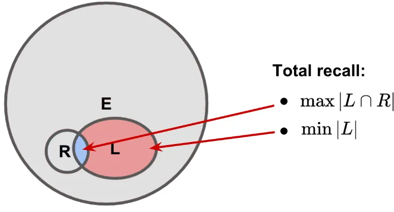
The total recall problem in information retrieval aims to optimize the cost for achieving very high recall–as close as practicable to 100%–with a human assessor in the loop [Gro16]. More specifically, the total recall problem can be described as follows, with a graph demonstration in Figure 2.1:
Given a set of candidatesE, in which only a small fractionR⊂E are positive, each candidate x ∈E can be inspected to reveal its label as positive (x∈R) or negative (x6∈R) at a cost. Starting with the labeled setL=;, the task is to inspect and label as few candidates as possible (min|L|) while achieving very high recall (max|L∩R|/|R|).
The Total Recall Problem:
2.2
Motivation
Figure 2.1The Total Recall Problem.
2.2.1 Electronic Discovery
Electronic Discovery (e-discovery) is a part of civil litigation where one party (the producing party), offers up materials which are pertinent to a legal case [Kri16]. This involves a review task where the producing party need to retrieve every “relevant” document in their possession and turn them over to the requesting party. It is extremely important to reduce the review cost in e-discovery since in a common case, the producing party will need to retrieve thousands of “relevant” documents among millions of candidates. To reduce the amount of effort spent in examining documents, researchers from legal domains explore the problem as a total recall problem [CG15; GC13; CG14; GC13; CG17; CG16a; CG16b] with: • E: set of candidate documents.
• R: set of relevant documents to the legal case.
• L: set of documents that have been examined and labeled as relevant or non-relevant by attorneys.
2.2.2 Evidence-based Medicine
In evidence-based medicine, researchers screen titles and abstracts to determine whether one paper should be included in a certain systematic review. To reduce the amount of human effort spent in screening titles and abstracts, researchers from medicine explore the problem as a total recall problem [Wal10b; Wal10a; Wal11; WD12; Wal13a; Wal12; Wal13b; Ngu15; Miw14] with:
• E: set of papers returned from a search query. • R: set of relevant papers to the systematic review.
2.2.3 Primary Study Selection
For the same reason of medicine researchers, software engineering researchers also need to read literature to stay current on their research topics. Researchers conduct systematic literature reviews [Kit04b] to analyze the existing literature and to facilitate other researchers. Among different steps of systematic literature reviews, primary study selection is in exactly the same format as citation screening in medical systematic reviews. The problem is also for reading titles and abstracts to find relevant papers to include, except that those papers are about software engineering. As a result, the primary study selection problem can be described as a total recall problem:
• E: set of papers returned from a search query.
• R: set of relevant papers to the systematic literature review.
• L: set of papers that have been reviewed and labeled as relevant or non-relevant by human researchers. In Chapter 3, we will demonstrate how our FASTREAD approach solves the total recall problem with primary study selection as case studies.
2.2.4 Test Case Prioritization
Regression testing is an expensive testing process to detect whether new faults have been introduced into previously tested code. To reduce the cost of regression testing, software testers may prioritize their test cases so that those which are more likely to fail are run earlier in the regression testing process [Elb02]. The goal of test case prioritization is to increase the rate of fault detection, and by doing so, it can provide earlier feedback on the system under test, enable earlier debugging, and increase the likelihood that, if testing is prematurely halted, those test cases that offer the greatest fault detection ability in the available testing time will have been executed [Elb02]. This test case prioritization problem can also be treated as a total recall problem with the following notations:
• E: all candidate regression test suites. • R: set of test suites that will detect faults. • L: set of test suites that have been executed.
Existing techniques for prioritizing test cases are “unsupervised”, i.e. these techniques decide an order of the test cases to be run and stick with it. Applying active learning to adapt the ordering with knowledge learned from test cases executed can potentially further increase the rate of fault detection and reduce more cost. However, this problem has not been explored as a total recall problem and the following challenges need to be resolved:
• What types of feature can be extracted from the test cases so that the learned model can accurately predict the likelihood of fault detection from a test case before its execution.
• How to balance the priority of test cases increasing coverage of statements/functions most and the more-likely-to-fail test cases.
2.2.5 Software Security Vulnerability Prediction
Society needs more secure software. It is crucial to identify software security vulnerabilities and fix them as early as possible. However, it is time-consuming to have human experts inspecting the entire codebase looking for the few source code files that contain vulnerabilities. The solution to this problem, prioritizing the human inspection effort towards codes that are more likely to have vulnerabilities is also a total recall problem:
• E: the entire codebase of a software project.
• R: set of source code files that contain vulnerabilities.
• L: set of source code files already inspected by human engineers.
2.3
Challenges of Total Recall Problem
Given that all the above problems in Section 2.2 can be generalized as the total recall problem, it is beneficial if we can better solve the total recall problem. In the rest of this section, we present the four important challenges for solving the total recall problem.
2.3.1 Higher Recall and Lower Cost
As mentioned in Section 2.1, the core challenge of the total recall problem is to achieve higher recall (max|L∩R|/|R|) with lower cost (min|L|).
2.3.1.1 Related work
Different strategies have been applied to solve the higher recall and lower cost challenge, includ-ing supervised learninclud-ing [Coh06; Ade14], unsupervised learninclud-ing [Mal07; Fel10], and semi-supervised learning [Cha17]. However, the state of the art solutions to the total recall problem apply active learn-ing [Gro16].
Figure 2.2Power of active learning on total recall problems.
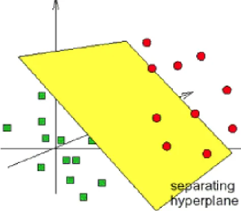
Figure 2.3Separating relevant (red) artifacts from non-relevant (green) artifacts.
When solving the total recall problem, the state of the art solutions apply active learning to learn from natural language processing features (e.g. bag-of-words, tf-idf) extracted from the current labeled setL and re-rank the rest of the candidatesE \Lso that candidates that are more likely to be positive get inspected next. This active learning solution has been proven effective in different use cases. A demonstration of the benefit of this active learning strategy can be found in Figure 2.2, where with active learning (solid red line), high recall (close to 100%) can be achieved by inspecting only a small portion of the candidates.
In electronic discovery, Cormack and Grossman [CG14] proposed continuous active learning to save attorneys’ effort from reviewing non-relevant documents, which further can save a large amount of the cost of legal cases.
In evidence-based medicine, Wallace et al. [Wal10b] designed patient active learning to help re-searchers prioritize their effort on papers to be included. With patient active learning, half of the screening effort can be saved while still including most relevant papers [Wal10b]. Miwa et al. [Miw14] then applied certainty sampling based active learning to achieve better performance than patient active learning.
The active learning strategy for total recall problem can be described as following: Step 0 Given a candidate setE and initialize the labeled setL=;.
Step 1 Using strategies like ad hoc search or random sampling to select next example x to label (L←L∪x).
Step 2 RepeatStep 1until “enough” positive examples have been labeled (|L∩R| ≥K). Step 3 Train/update a supervised learning model with current labeled setL.
Step 4 Use the trained model to predict on the unlabeled setE\L and select next examplex to label (L←L∪x).
Step 5 RepeatStep 3andStep 4until the stopping rule is met. Where detail settings vary from case studies to case studies:
• InStep 2, Cormack and Grossman [CG14] believe learning should start as soon as possible (K =1) while Wallace et al. [Wal10b] suggest to start learning until more training examples are available. • InStep 3, most studies exact text features from examples and train a support vector machine with
linear kernel. However, there are different opinions on how to balance the training data, e.g. Wallace et al. [Wal10b] proposed a technique called aggressive undersampling to drop off the negative examples closes to the positive ones while Miwa et al. [Miw14] adjusted the weight of each training example to punish more for misclassifying positive examples.
• InStep 4, Cormack and Grossman [CG14] select examples that are most likely to be positive while Wallace et al. [Wal10b] select most uncertain examples.
• InStep 5, Cormack and Grossman [CG14] stop the process when a sufficient number of positive examples have been found while Wallace et al. [Wal10b] stop the learning when the model becomes stable and then apply the model to classify the unlabeled examples.
2.3.1.2 Performance metrics
When assessing how well an approach solves the higher recall and lower cost challenge, therecall (|LR|/|R|)vs.cost (|L|)curve is usually applied. This performance metrics is suggested by Cormack et al. [CG15; CG14; Tre15] and best evaluates the performance of different approaches. To enable a statistical analysis of the performances, therecallvs.costcurve is always cut by a0.95recallline where cost at0.95recall—X95—is used to assess performances. The reason behind0.95recallis that a)1.00 recallcan never be guaranteed by any approach unless all the candidatesE are reviewed; b)0.95recall is usually considered acceptable [Coh11; Coh06; OE15] despite the fact that there might still be “relevant” artifacts missing [She16]. As a result, two metrics are used for evaluation:
• X95 =min{|L| | |LR| ≥0.95|R|}. • WSS@95 =0.95−X95/|P|.
Note that one algorithm is better than the other if its X95 is smaller or WSS@95 [Coh11] is larger. As recommended by Mittas & Angelis in their 2013 IEEE TSE paper [MA13], Scott-Knott analy-sis was applied to cluster and rank the performance (X95 or WSS@95) of each treatment. It clusters treatments with little difference in performance together and ranks each cluster with the median per-formances [SK74]. Nonparametric hypothesis tests are applied to handle the non-normal distribution. Specifically, Scott-Knott decided two methods are not of little difference if both bootstrapping [Efr82], and an effect size test [Cli93] agreed that the difference is statistically significant (99%confidence) and not a negligible effect (Cliff’s Delta≥0.147).
2.3.2 When to Stop
In practice, there is no way to know the number of positive examples before inspecting and labeling every candidate example. It is thus impossible to know exactly what recall has been reached during the process. Then, how do we know when to stop if the target is reaching, say 95% recall? This is a practical problem that directly affects the usability of the active learning strategy. Stopping too early will result in missing many valuable positive examples; while stopping too late will cause unnecessary cost when there are no more positive examples to retrieve.
2.3.2.1 Related work
So far, researchers have developed various stopping rules to solve the “when to stop” problem.
• Ros et al. [Ros17] developed the the most straightforward rule, which decides that the process should be stopped after 50 negative examples are found in succession.
• Cormack and Grossman proposed the knee method [CG16a], which detects the inflection pointi of current recall curve, and compare the slopes before and afteri. Ifs l o p e<i/s l o p e>i is greater than a specific thresholdρ, the review should be stopped.
2.3.2.2 Performance metrics
Later in Chapter 3 we will show that, similarly as Wallace et al. [Wal13a], we decide when to stop by estimating the number of positive examples|R|with|RE|. We use the Estimation vs Cost curve to assess the accuracy for the estimation, here
estimation=|RE|
|R| . (2.1)
The sooner this estimation converges to 1.0, the better the estimator is. As described in Step 7, the inspection process will stop when
|LR| ≥Tr e c|RE|,
whereTr e c represents the target recall. The closer the inspection stops to the target recall, the better the stopping rule.
2.3.3 Human Error Correction
When solving the total recall problems, the next example to be inspected relies on model trained on previously labeled examples. What if those labels can be wrong? The trained model could be misled by wrongly labeled examples and thus make worse decision on which example to inspect next.
2.3.3.1 Related work
By now, researchers have applied various strategies to correct such human errors:
• One simple way to correct human errors is by majority vote [Kuh17], where every example will be inspected by two different humans, and when the two humans disagree with each other, a third human is asked to make the final decision.
• Cormack and Grossman [CG17] built an error correction method upon the knee stopping rule [CG16a]. After the review stops, examples labeled as positive but are inspected after the inflection point (x>i) and examples labeled as negative but inspected before the inflection point (x<i) are sent to humans for a recheck.
2.3.3.2 Performance metrics
We still use cost and recall to assess the performance of different approaches when human errors are included in the experiment, except that this time:
c o s t =|L
0
|
|E| (2.2)
r e c a l l=t p
|R| (2.3)
2.3.4 Scalability
How to scale up the active learning framework with multiple humans working simultaneously on the same project remains an open challenge to the total recall problem.
2.3.4.1 Related work
In electronic discovery, Cormack and Grossman [CG16b] proposed S-CAL where model trained on a finite number of examples is used to predict and estimate the precision, recall, and prevalence of the target large set of examples. However, this approach sacrifices the adaptability of the active learner. In evidence-based medicine, Nguyen et al. [Ngu15] explored the task allocation problem where two types of human operators are available: (1) crowdsourcing workers who are cheaper but less accurate, and (2) experts who are much more expensive but also more accurate. This approach allows the system to operate more economically but still cannot scale up with growing number of training examples.
2.3.4.2 Performance metrics
We have not started exploring this challenge yet but thetraining time vs.training size curve will be applied to assess the scalability of different approaches.
2.4
Summary
CHAPTER
3
FASTREAD
This chapter describes FASTREAD, an active learning-based framework for solving the total recall problem described in Chapter 2. So far, FASTREAD has targeted on and solved three challenges of the total recall problem (higher recall and lower cost, when to stop, human error correction) and we plan to explore the last challenge (scalability) in our future work before graduation.
3.1
FASTREAD Operators
Using active learning as the general strategy, FASTREAD applies seven operators to solve the challenges of the total recall problem. This section offers an overview of these seven operators.
Featuresare not restricted in FASTREAD. Any types of features extracted from the software artifacts can be used to predict for relevancy in FASTREAD. That said, users could extract their own features
Support vector machines (SVMs)are a well-known and widely-used classification technique. The idea behind SVMs is to map input data to a high-dimension feature space and then construct a linear decision plane in that feature space [CV95]. Soft-margin linear SVM [Joa06] has been proved to be a useful model in SE text mining [Kri16] and is applied in the state-of-the-art total recall methods [Miw14; Wal10b; CG14].
Aggressive undersamplingis a data balancing technique first created by Wallaceet al.[Wal10b]. During the training process, aggressive undersampling throws away majority (non-relevant) training examples closest to SVM decision plane until reaching the same number of minority (relevant) training examples.
presumptive non-relevant examplessamples randomly from the unlabeled examples and presumes the sampled examples to be non-relevant (non-relevant) in training. The rationale behind this technique is that given the low prevalence of relevant (relevant) examples, it is likely that most of the presumed ones are non-relevant (non-relevant).
Query strategyis the key part of active learning. The two query strategies applied in this paper are: 1)uncertainty sampling, which picks the unlabeled examples that the active learner is most uncertain about (examples that are closest to the SVM decision hyperplane); and 2)certainty sampling, which picks the unlabeled examples that the active learner is most certain to be relevant (examples on the relevant side of and are furthest to the SVM decision hyperplane). Different approaches endorse different query strategy, e.g. Wallaceet al.[Wal10b] applies uncertainty sampling in their patient active learning, Cormacket al.[CG14; Miw14] use certainty sampling from beginning to the end. FASTREAD applies uncertainty sampling in early stage and certainty sampling afterwards.
SEMIis a semi-supervised estimator we designed for reading research papers [YM19]. SEMI utilizes a recursiveTemporaryLabel technique. Each time the SVM model is retrained, SEMI assigns temporary labels to unlabeled examples and builds a logistic regression model on the temporary labeled data. It then uses the obtained regression model to predict on the unlabeled data and updates the temporary labels. This process is iterated until convergence and the final temporary labels are used as an estimation of the total number of positive examples in the dataset.
DISAGREEis an error correction mechanism designed for correcting both false negatives and false positives [YM19]. Its core assumption is:
Human classification errors are more likely to be found where human and machine classifiers disagree most.
3.2
FASTREAD Framework
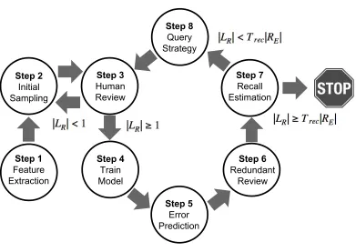
As shown in Figure 3.1, FASTREAD follows the procedures below, with the seven operators from §3.1 in bold:
Step 1 Feature Extraction:Given a set of candidate research papersC from searching, extractfeatures from each paper. Initialize the set of labeled papers asL← ;and the set of labeled relevant papers asLR ← ;.
Step 2 Initial Sampling: Sample without replacementN1 unlabeled candidate papers to generate a
queueQ⊂(C \L)1, (a) randomly, if not using any domain knowledge; or (b) following the guidance of domain knowledge.
Step 3 Human Review:Each human is assigned one random paper from the queuex∈Q; label it as “relevant” or “non-relevant” after reviewing it. Add paperx into the labeled setL; ifx is labeled “relevant” also add it into setLR. The human is then assigned another paper until the queue is
1LetAandBbe two sets. The set difference, denotedA\Bconsists of all elements ofAexcept those which are also elements
Step 2 Initial Sampling
Step 3 Human Review
Step 4 Train Model
Step 6 Redundant
Review Step 7
Recall Estimation Step 8
Query Strategy
Step 1 Feature Extraction
Step 5 Error Prediction
Figure 3.1The FASTREAD framework.
cleared. Once the queue is cleared, proceed toStep 4to start training if at least one “relevant” paper is found (|LR| ≥1), otherwise go back toStep 2to sample more.
Step 4 Train Model:Generatepresumptive non-relevant examplesto alleviate the sampling bias in “non-relevant” examples (L\LR). Applyaggressive undersamplingto balance the training data. At last train a linearsupport vector machine(SVM) on the current labeled papersLR andL, using features extracted inStep 1to predict whether one paper is relevant or not.
Step 5 Error Prediction (DISAGREE): Apply theSVM model trained inStep 4to predict on the papers that have only been reviewed once and are labeled as “non-relevant” (L\LR). SelectN2
papers with highest prediction probability of being relevant and add the selected papers into a queue for redundant reviews.
Step 6 Redundant Review:Each paper in the queue fromStep 5is assigned to different humans other than its original reviewer for redundant review. Once the queue is cleared, proceed toStep 7. Step 7 Recall Estimation: Estimate the total number of relevant papers|RE|withSEMIalgorithm.
• STOPthe review process if|LR| ≥Tr e c|RE|(whereTr e c represents the user target recall). • Otherwise proceed toStep 8.
Step 8 Query Strategy:Apply theSVMmodel trained inStep 4to predict on unlabeled papers(C\L) and select topN papers with prediction probability closest to0.5 (uncertainty sampling) if
then go toStep 3for another round of review.
In the above,N1,N2,N3are engineering choices.N1is the batch size of the review process, larger batch
size usually leads to fewer times of training but also worse overall performance.N2=αN1whereα∈[0, 1] reflects what percentage of the labeled files are redundantly reviewed. LargerN2means more redundant
review effort, which leads to more human false positives covered by also higher cost.N3is the threshold
where the query strategy is switched from uncertainty sampling to certainty sampling.N3features the trade-off between faster building a better model and greedily applying the model to save human review effort.
3.3
Summary
CHAPTER
4
CASE STUDY #1: FINDING RELEVANT
RESEARCH PAPERS
In this section, we will demonstrate how FASTREAD is designed and how it solves the three challenges of total recall problem when finding relevant research papers to a certain topic.
4.1
Introduction
Why is it important to reduce the effort associated with finding the relevant research papers? Given the prevalence of tools like SCOPUS, Google Scholar, ACM Portal, IEEE Xplorer, Science Direct, etc., it is a relatively simple task to find a few relevant papers for any particular research query. However, what if the goal is not to find afewpapers, but instead to findmostof the relevant papers? Such broad searches are very commonly conducted by:
• Researchers exploring a new area;
• Researchers writing papers for peer review, to ensure reviewers will not reject a paper since it omits important related work;
• Researchers conducting a systematic literature review on a specific field to learn about and summarize the latest developments.
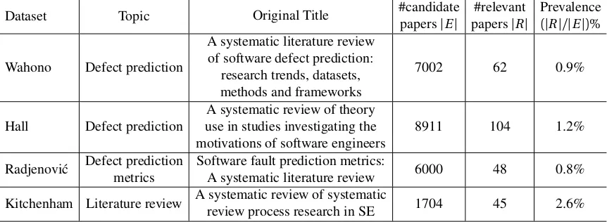
Table 4.1Statistics from the literature review case studiesr
Dataset Topic Original Title #candidate
papers|E|
#relevant papers|R|
Prevalence
(|R|/|E|)%
Wahono Defect prediction
A systematic literature review of software defect prediction:
research trends, datasets, methods and frameworks
7002 62 0.9%
Hall Defect prediction
A systematic review of theory use in studies investigating the motivations of software engineers
8911 104 1.2%
Radjenovi´c Defect prediction metrics
Software fault prediction metrics:
A systematic literature review 6000 48 0.8%
Kitchenham Literature review A systematic review of systematic
review process research in SE 1704 45 2.6%
Datasets used in the chapter. The first three datasets are generated by reverse engineering from the original publications (using the same search string to collect candidate papers and treating the final inclusion list as ground truth for relevant papers).
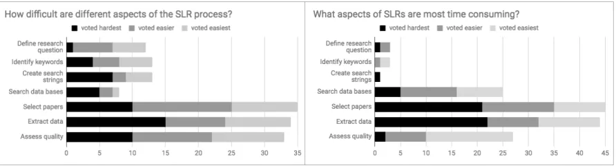
literature review, which is called primary study selection, is to find most (if not all) of the relevant papers to the research questions. This step is identified as one of the most difficult and time consuming steps in systematic literature review [Car13] as it requires humans to read and classify thousands of candidate papers from a search result. Table 4.1 shows four systematic literature reviews where thousands of papers were reviewed before revealing just a few dozen relevant papers. Shemilt et al. [She16] estimated that assessing one paper for relevancy takes at least one minute. Assuming 25 hours per week for this onerous task, the studies of Table 4.1 would take 16 weeks to complete (in total). Therefore, reducing the human efforts required in this primary study selection step is thus critical for enabling researchers conducting systematic literature reviews more frequently.
Many researchers have tried reducing the effort associated with literature reviews [Mal07; Bow12; JW12; Woh14; OE15; Pay16; Coh06; Ade14; Liu16; Ros17]. Learning from those prior works, an active learning-based solution called FASTREAD is proposed to address this problem. FASTREAD addresses the first three challenges of the total recall problem by answering the research questions defined in §1.2: RQ1: “Higher recall and lower cost”; i.e., how to better select which paper to review next, so that most relevant papers can be found by reviewing least amount of papers. By mixing and matching the prior state of the art solutions to this challenge, we found one combination that outperformed all the rest including the state of the art solutions. FASTREAD then adopts that combination as the most efficient way to find relevant papers fast.
Figure 4.1This chapter explores tools for reducing the effort and difficulty associated with theselect papers
phase of systematic literature reviews. We do this since Carver et al. [Car13] polled researchers who have con-ducted literature reviews. According to their votes,select paperswas one of the hardest, most time-consuming tasks in the literature review process. For tools that support other aspects of SLRs such as searching databases and extracting data, see summaries from Marshall et al. [Mar15].
RQ2: “When to stop”; i.e., how to know when can the review be safely stopped. While there is probably always one more relevant paper to find, it would be useful to know when most papers have been found (say, 95% of them [Coh11]). Without the knowledge of how many relevant papers that are left to be found, researchers might either:
• Stop too early, thus missing many relevant papers.
• Stop too late, causing unnecessary further reading, even after all relevant items are find.
In the FASTREAD approach, the current achieved recall of relevant papers can be accurately estimated through a semi-supervised logistic regressor. Therefore it is possible to determine when a target recall (say, 95%), has been reached. We show, in §4.6.4 that our stopping rule is more accurate than other state of the art stopping criteria [Wal13a].
RQ3: “Human error correction”. Human reviewers are not perfect, and sometimes they will label relevant papers as non-relevant, and vice versa. Practical tools for support literature reviews must be able to recognize and repair incorrect labeling. We show that in FASTREAD, the human labeling errors can be efficiently identified and corrected by periodically rechecking part of the labeled papers, whose labels the active learner disagrees most on.
4.2
Background
4.2.1 Literature Reviews in Different Domains
Selecting which technical papers to read is a task that is relevant and useful for many domains. For example:
• In legal reasoning, attorneys are paid to review millions of documents trying to find evidence to some case. Tools to support this process are referred to aselectronic discovery[GC13; CG14; CG15; CG16b]. • In evidence-based medicine, researchers review medical publications to gather evidence for support
of a certain medical practice or phenomenon. The selection of related medical publications among thousands of candidates returned by some search string is called citation screening. Text mining methods are also applied to reduce the review effort in citation screening [Miw14; Wal10b; Wal10a; Wal11; Wal13a; Wal12; Wal13b].
• In software engineering, Kitchenhamet al. recommendsystematic literature reviews(SLRs) to be standard procedure in research [Kit04b; Kee07]. In systematic literature reviews, the process of selecting relevant papers is referred to as primary study selection when SE researchers review titles, abstracts, sometimes full texts of candidate research papers to find the ones that are relevant to their research questions [Kit04a; Kee07].
For the most part, SLRs in SE are a mostly manual process (evidence: none of the researchers surveyed in Fig 4.1 used any automatic tools to reduce the search space for their reading). Manual SLRs can be too slow to complete or repeat. Hence, the rest of this chapter explores methods to reduce the effort associated with literature reviews.
4.2.2 Automatic Tool Support
Tools that address this problem can be divided as follows:
Search-query based that involves query expansion/rewriting based on user feedback [Ume16]. This is the process performed by any user as they run one query and reflect on the relevancy/irrelevancy of the papers returned by (e.g.) a Google Scholar query. In this search-query based approach, users struggle to rewrite their query in order find fewer non-relevant papers. While a simple method to manually rewrite search queries, its performance in selecting relevant papers is outperformed by the abstract-based methods described below [Goe17; Kan17].
Table 4.2Problem description
E: the set of all candidate papers (returned from search). R⊂E: set of ground truth relevant papers.
I =E \R: set of ground truth non-relevant papers
L⊂E: set of labeled/reviewed papers, each review reveals whether a paper is included or not.
¬L=E \L: set of unlabeled/unreviewed papers. LR=L∩R: identified relevant (included) papers. LI =L∩I: identified non-relevant (excluded) papers.
Abstract based methods use text from a paper’s abstract to train text classification models, then apply those models to support the selection of other relevant papers. Since it is easy to implement and performs reliably well, abstract-based methods are widely used in many domains [Yu18; Miw14; Wal10b; CG14].
4.2.3 Abstract-based Methods
In this chapter, we focus onabstract-based methods since:
• They are easy to implement—the only extra cost is some negligible training time, compared to search query based methods which require human judgments on keywords selection and reference based methods which cost time and effort in extracting reference information.
• Several studies show that the performance of abstract-based methods is better than other approaches [Kan17; Roe15].
Note that abstract-based methods do not restrict the reviewers from making decisions based on full-text when it is hard to tell whether one paper should be included or not based on abstract. However, only abstracts are used for training and prediction, which makes data collection much easier. Abstract-based methods utilize different types of machine learning algorithms :
1. Supervised learning: which trains on labeled papers (that humans have already labeled as relevant/non-relevant) before classifying the remaining unlabeled papers automatically [Coh06; Ade14]. One problem with supervised learning methods is that they need a sufficiently large labeled training set to operate and it is extremely inefficient to collect such labeled data via random sampling. For this reason, supervised learners are often combined with active learning (see below) to reduce the cost of data collection.
2. Unsupervised learning: techniques like visual text mining (VTM) can be applied to facilitate the human labeling process [Mal07; Fel10]. In practice the cost reductions associated with (say) visual text mining is not as significant as that ofactive learningmethods due to not utilizing any labeling information [Roe15; Kan17].
sets–Liu et al. [Liu16] reported a less than 95% recall with 30% data labeled).
4. Active learning: In this approach, human reviewers read a few papers and classify each one as relevant or non-relevant. Machine learners then use this feedback to learn their models incrementally. These models are then used to sort the stream of papers such that humans read the most informative ones first.
In this chapter, we explore the active learning-based approach since it has been shown as most effective in prior state of the art works [Gro16; Roe15].
4.3
Datasets
Although a large number of SLRs are published every year, there is no dataset clearly documenting the details in primary study selection. As a result, three datasets are created reverse-engineering existing SLRs and being used in this study to simulate the process of excluding irrelevant studies. The three datasets are named after the authors of their original publication source– Wahono dataset from Wahono et al. 2015 [Wah15], Hall dataset from Hall et al. 2012 [Hal12], and Radjenovi´c dataset from Radjenovi´c et al. 2013 [Rad13].
For each of the datasets, the search string and the final inclusion listFfrom the original publication are used for the data collection. We retrieve the initial candidate collectionEfrom IEEE Xplore with the search string (slightly modified to meet the requirement of IEEE Xplore). Then make a final list of inclusionRasR=F∩E. Here, for simplicity we only extract candidate studies from IEEE Xplore. We will explore possibilities for efficiently utilizing multiple data sources in the future work but in this paper, without loss of generality, we only extract initial candidate list from single data source. In this way, we created three datasets that reasonably resemble real SLR selection results assuming that any study outside the final inclusion listFis irrelevant to the original SLRs. A summary of the created datasets is presented in Table 4.1.
Apart from the three created datasets, one dataset (Kitchenham) is provided directly by the author of Kitchenham et al. 2010 [Kit10] and includes two levels of relevance information. In general, only the “content relevant” labels are used in experiments for a fair comparison with other datasets.
All the above datasets are available on-line at Seacraft, Zenodo1.
4.4
Higher recall and lower cost
This section focuses on the higher recall and lower cost challenge of the total recall problem. Our proposed approach FASTREAD greatly benefits from the prior state of the art solutions from electronic discovery and evidence-based medicine.
4.4.1 Related work
4.4.1.1 Legal Electronic Discovery Tools
In electronic discovery, attorneys are hired to review massive amount of documents looking for relevant ones for a certain legal case and provide those as evidences. Various machine learning algorithms have been studied to reduce the amount of effort spent in examining documents. So far, in every controlled studies, continuous active learning (Cormack’14) has outperformed others [CG14; CG15], which makes it the state-of-the-art method in legal electronic discovery. It has also been selected as a baseline method in the total recall track of TREC 2015 [Roe15]. Details on continuous active learning are provided in §4.4.2.
4.4.1.2 Evidence-based Medicine Tools
Systematic literature reviews were first adopted from evidence-based medicine in 2004 [Kit04b]. To facilitate citation screening (primary study selection) in systematic review, many groups of researchers have investigated different types of machine learning algorithms and evaluation mechanisms [OE15; Pay16].
Wallace et al. conducted a series of studies with machine learning techniques, especially active learn-ing [Wal10b; Wal10a]. Wallace set up a baseline approach called “patient active learnlearn-ing” (Wallace’10) for machine learning assisted citation screening [Wal10b]. The performance of patient active learning is good enough (nearly 100% of the “relevant” citations can be retrieved at half of the conventional review cost) to convince systematic review conductors to adopt machine learning assisted citation screening.
More recent work of Miwa et al. explored alternative data balancing and query strategy in 2014 [Miw14] and proposed a new treatment of Certainty plus Weighting (Miwa’14). Instead of uncertainty sampling in patient active learning (Wallace’10), Miwa found that certainty sampling provides better results in clinical citation screening tasks. Similar conclusion for data balancing method as weighting relevant examples was found to be more effective than aggressive undersampling. Although not stated explicitly, Certainty plus Weighting keeps training until all “relevant” studies have been discovered, which differs from the stopping criteria of Wallace’10. Aside from the core algorithm, additional views from latent Dirichlet allocation (LDA) has been found to be potentially useful.
Details on the above two state of the art solutions are provided in §4.4.2.
4.4.2 Methodology
As mentioned in §4.2, the existing state-of-the-art methods are Wallace’10 [Wal10b] (patient active learning), Miwa’14 [Miw14] (Certainty plus Weighting), and Cormack’14 [CG14] (continuous active learning). All three state-of-the-art methods share the following common techniques.
(a)No data balancing (b)With weighting (c)With aggressive undersampling.
Figure 4.2Active learning with SVM and different data balancing techniques.
text mining [Kri16] and is applied in the state-of-the-art active learning methods of both evidence-based medicine and electronic discovery [Miw14; Wal10b; CG14]. One drawback of SVM is its poor interpretability as compared to classifiers like decision trees. However, SVM still fits here since the model itself is not important as long as it could provide a relative ranking of literature.
Active learningis a cost-aware machine learning algorithm where labels of training data can be acquired with certain costs. The key idea behind active learning is that a machine learning algorithm can perform better with less training if it is allowed to choose the data from which it learns [Set12]. There are several scenarios active learning is applied to, such as membership query synthesis, stream-based selective sampling, and pool-based sampling [Set10]. There are also different query strategies of active learning, such as uncertainty sampling, query-by-committee, expected model change, expected error reduction, variance reduction, and density-weighted methods [Set10]. Here, we briefly introduce one scenario and two query strategies, which are used in our later experiments and discussions.
Figure 4.2 shows a simple demonstration of an SVM active-learner. For the sake of simplicity, this demonstration assumes that the data has two features (shown in that figure as the horizontal and vertical axis). In that figure, “O” is the minority class, “relevant” studies in SLR. “O”s in blue are studies already identified as “relevant” (included) by human reviewers. “X” is the majority class, “irrelevant” studies in SLR. “X”s in red are studies already identified as “irrelevant” (excluded) by human reviewers (note that in (c), some red “X”s are removed from the training set by aggressive undersampling). Markers in gray are the unlabeled studies (studies have not been reviewed yet), and black line is SVM decision plane. In (b) Weighting balances the training data by putting more weight on the minority class examples. In (c), aggressive undersampling balances the training data by throwing away majority class examples closest to the old decision plane in (a). When deciding which studies to be reviewed next, uncertainty sampling returns the unlabeled examples closest to the decision plane (U) while certainty sampling returns the unlabeled examples furthest to the decision plane from the bottom-left side (C).
By analyzing the differences between the state-of-the-art methods, we identified the following key components in solving the problem with active learning and linear SVM.
• Pstands for “patient”. As suggested by Wallace et al. [Wal10b], “hasty generation”, which means start training with too few relevant examples, may lead to poor performance. The algorithm keeps random sampling until a sufficient number of “relevant” studies are retrieved. In our experiments, the sufficient number of “relevant” studies retrieved is set to5, which means when at least5“relevant” studies have been retrieved by random sampling, the algorithm goes into next stage. Wallace’10 [Wal10b] and Miwa’14 [Miw14] usePfor when to start training.
• Hstands for “hasty”, which is the opposite ofP. The algorithm starts training as soon asONE“relevant” study is retrieved, as suggested in Cormack’14 [CG14; CG15].
Which document to query next:
• Ustands for “uncertainty sampling”. The algorithm utilizes uncertainty sampling to build the classifier, where unlabeled examples closest to the SVM decision plane are sampled for query (U in Figure 4.2). Wallace’10 [Wal10b] usesUfor Query strategy.
• Cstands for “certainty sampling”. The algorithm utilizes certainty sampling to build the classifier, where unlabeled examples furthest to the SVM decision plane and lie in the “relevant” side are sampled for query (C in Figure 4.2). Miwa’14 [Miw14] and Cormack’14 [CG14; CG15] use Cfor query strategy.
Whether to stop training (or not):
• Sstands for “stop training”. The algorithm stops training once the classifier is stable. In our experiments, the classifier is treated as stable once more than30“relevant” studies have been retrieved as training examples. Wallace’10 [Wal10b] usesSfor whether to stop training.
• Tstands for “continue training”. The algorithm never stops training as suggested in Cormack’14 [CG14] and Miwa’14 [Miw14]. If query strategy isU, algorithm switches to certainty sampling after classifier is stable but training never stops.
How to balance the training data:
• Nstands for “no data balancing”. The algorithm does not balance the training data (demonstrated in Figure 4.2a) as suggested by Cormack’14 [CG14].
• Astands for “aggressive undersampling”. The algorithm utilizes aggressive undersampling2 after
classifier is stable, as suggested by Wallace’10 [Wal10b].
• Wstands for “Weighting”. The algorithm utilizes Weighting3for data balancing (before and after the classifier is stable), as suggested by Miwa’14 [Miw14].
• M stands for “mixing of Weighting and aggressive undersampling”. Weighting is applied before the classifier is stable while aggressive undersampling is applied after the classifier is stable. This treatment comes from the observation that “Weighting” performs better in early stages while “aggressive undersampling” performs better in later stages.
By combining different approaches, we ended up with 32 possible treatments including the state-of-the-art methods:
2Aggressive undersampling throws away majority (irrelevant) training examples closest to SVM decision plane until reaching
the same number of minority (relevant) training examples. A demonstration is shown in Figure 4.2c.
3Weighting assigns different weight to each class,W
• ThePUSAapproach advocated by Wallace’10 [Wal10b]. • ThePCTWapproach advocated by Miwa’14 [Miw14]. • TheHCTNapproach advocated by Cormack’14 [CG14].
4.4.3 Experiments
In this subsection, we design experiments to answerRQ1by comparing all 32 machine learning treatments along with the current standard procedure as a baseline treatment—Linear Review: no machine learning, query studies in a random order.
4.4.3.1 Simulation Studies
In the following, each experiment is a simulation of one specific treatment on one dataset. More specifically, there is no human activity involved in these experiments, when asked for a label, the true label in the dataset is queried instead of a human reviewer. As a result, each experiment can be repeated with different random seed to capture variances and also makes reproducing the experiments possible.
4.4.3.2 Controlled Variables
For the sake of a fair comparison, different treatments in §4.4.2 share an identical set of controlled variables including preprocessing, featurization and classifier.
Each candidate study in the initial list is first tokenized by stop words removal after concatenating its title and abstract. After tokenization, the bag of words are featurized into a term frequency vector. Then, reduce the dimensionality of the term frequency vector with to keep onlyM =4000of the terms with highest tf-idf4score and normalize the hashed matrix by its L2 norm each row at last. TfidfVectorizer in scikit-learn is utilized for the above preprocessing and featurization steps. Alternatives such as stemming, LDA [Ble03], paragraph vectors [LM14] require further exploration and are scheduled in our future works. All 32 treatments use the same classifier– linear SVM from scikit-learn.
4.4.4 Results
All the following results were generated from 30 repeats simulations, using different random number seeds from each simulation. As shown below, all our results are reported in terms of medians (50th percentile) and iqrs ((75-25)th percentile).
RQ1: “Higher recall and lower cost”.
In Table 4.3, performance of the three state-of-the-art treatments are colored in red . On Wahono datasets, Miwa’14 (PCTW) outperforms the other two treatments; while on Hall dataset, Cormack’14 (HCTN) has the best performance; on Radjenovi´c dataset, all three treatments perform similarly; and on Kitchenham dataset, Wallace’10 (PUSA) outperforms the others. Neither of the three state-of-the-art treatments consistently performs the best. This means that adopting the state-of-the-art treatments will
4For termtin documentd,T f i d f(t,d) =wt d×(log
|D|
P
d∈Ds g n(wdt)+
1)wherewt
i is the term frequency of termt in document d. For termt,T f i d f(t) =P
T f i d f(t,d) =P
wt×(log |D| +
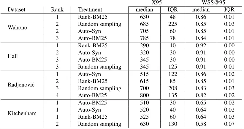
Table 4.3Scott-Knott analysis for number of studies reviewed/ work saved over sampling to reach95%recall
Wahono X95 WSS@95
Rank Treatment Median IQR Median IQR
1 HUTM 670 230 0.85 0.04 1 HCTM 740 220 0.84 0.03 2 HUTA 780 140 0.84 0.02 2 HCTW 790 90 0.84 0.02 2 HUTW 800 110 0.84 0.02 2 HCTA 800 140 0.83 0.02 3 PCTM 1150 450 0.78 0.07 3 PUTM 1180 420 0.78 0.07 3 PCTA 1190 340 0.78 0.05 3 PUTA 1190 340 0.78 0.05 3 PCTW 1210 350 0.78 0.06 3 PUTW 1220 370 0.77 0.06 4 HUSM 1410 400 0.75 0.06 5 HUSA 1610 370 0.72 0.07 6 PUSM 1810 370 0.69 0.06 6 PUSA 1910 700 0.67 0.10 7 HUSW 2220 400 0.63 0.06 7 PUSW 2240 360 0.63 0.06 8 HUTN 2700 40 0.56 0.01 8 HCTN 2720 40 0.56 0.01 8 PCSW 2860 1320 0.54 0.20 8 PCSM 2860 1320 0.54 0.20 8 PCTN 2850 1130 0.54 0.17 8 PUTN 2850 1130 0.54 0.17 9 PCSN 3020 1810 0.51 0.26 9 PCSA 3020 1810 0.51 0.26 10 HUSN 4320 110 0.33 0.03 10 PUSN 4370 1290 0.32 0.19 11 linear 6650 0 0 0 11 HCSA 6490 2760 -0.01 0.39 11 HCSN 6490 2760 -0.01 0.39 11 HCSM 6490 3110 -0.01 0.44 11 HCSW 6490 3110 -0.01 0.44
Hall X95 WSS@95
Rank Treatment Median IQR Median IQR
1 HUTW 340 90 0.91 0.01 1 HUTA 340 130 0.91 0.02 1 HUTM 350 120 0.91 0.01 1 HCTW 370 60 0.91 0.01 2 HUTN 370 90 0.91 0.01 2 HCTM 380 100 0.91 0.01 2 HCTA 390 150 0.91 0.02 2 HCTN 410 80 0.90 0.01 3 HUSM 530 120 0.89 0.01 3 HUSW 560 250 0.89 0.03 3 PCTW 610 210 0.88 0.02 3 PUTW 610 220 0.88 0.03 4 HUSA 630 170 0.88 0.02 4 PCTN 650 220 0.88 0.03 4 PUTN 650 220 0.88 0.03 4 PUTM 670 220 0.87 0.03 4 PCTM 680 230 0.87 0.03 4 PCTA 700 210 0.87 0.03 4 PUTA 700 220 0.87 0.03 4 PUSW 740 230 0.87 0.03 5 PUSM 770 240 0.86 0.03 5 PUSA 880 270 0.85 0.04 6 PCSW 1150 570 0.82 0.07 6 PCSM 1150 570 0.82 0.07 7 PCSN 1530 1050 0.78 0.13 7 PCSA 1530 1050 0.78 0.13 7 PUSN 1550 1120 0.77 0.13 7 HUSN 1800 1020 0.74 0.11 8 HCSA 7470 5980 0.03 0.67 8 HCSN 7470 5980 0.03 0.67 8 linear 8464 0 0 0 8 HCSM 8840 6060 -0.04 0.68 8 HCSW 8840 6060 -0.04 0.68
Radjenovi´c X95 WSS@95 Rank Treatment Median IQR Median IQR
1 HUTM 680 180 0.83 0.03 1 HCTM 780 130 0.82 0.02 1 HCTA 790 180 0.82 0.03 1 HUTA 800 180 0.82 0.03 2 HUSA 890 310 0.80 0.06 2 HUSM 890 270 0.80 0.05 3 HUTW 960 80 0.79 0.02 3 HCTW 980 60 0.79 0.01 3 HUSW 1080 410 0.77 0.07 4 PCTM 1150 270 0.76 0.05 4 PUTM 1150 270 0.76 0.05 5 HUTN 1250 100 0.74 0.02 5 PCTA 1260 210 0.74 0.05 5 PUTA 1260 210 0.74 0.05 5 HCTN 1270 70 0.74 0.02 5 PUSM 1250 400 0.74 0.07 5 PUSW 1250 450 0.73 0.08 5 PUTW 1350 310 0.72 0.06 5 PCTW 1370 310 0.72 0.06 5 PUSA 1400 490 0.71 0.09 6 HUSN 1570 300 0.69 0.05 6 PCTN 1600 360 0.68 0.06 6 PUTN 1600 360 0.68 0.06 7 PUSN 1890 320 0.64 0.06 8 PCSW 2250 940 0.57 0.20 8 PCSM 2250 940 0.57 0.20 9 PCSN 2840 1680 0.47 0.31 9 PCSA 2840 1680 0.47 0.31 10 HCSA 5310 2140 0.07 0.36 10 HCSN 5310 2140 0.07 0.36 10 HCSM 5320 2200 0.02 0.37 10 HCSW 5320 2200 0.02 0.37 10 linear 5700 0 0 0
Kitchenham X95 WSS@95 Rank Treatment Median IQR Median IQR
1 HUSA 590 170 0.60 0.19 1 HUTA 590 80 0.60 0.06 1 HUSM 620 70 0.58 0.04 1 HUTM 630 110 0.58 0.07 1 PUSA 640 130 0.57 0.08 1 HUSW 640 140 0.57 0.09 2 HUTN 680 30 0.55 0.02 2 HCTA 680 100 0.55 0.08 2 PUSM 680 90 0.55 0.06 2 HCTM 680 110 0.55 0.07 2 PCTM 690 90 0.54 0.06 2 PUTM 690 70 0.54 0.05 2 PUTA 710 110 0.53 0.08 2 HUTW 710 20 0.53 0.02 3 PUSW 720 110 0.52 0.08 3 PCTA 720 100 0.52 0.08 3 HCTN 730 60 0.52 0.04 3 HCTW 750 60 0.51 0.04 3 PUTN 750 80 0.51 0.05 4 PCTN 750 80 0.51 0.05 4 PUTW 780 70 0.49 0.04 4 PCTW 780 150 0.49 0.09 5 PUSN 800 140 0.47 0.09 5 HUSN 870 280 0.43 0.16 6 PCSW 990 330 0.35 0.19 6 PCSM 990 330 0.35 0.19 6 PCSN 1050 370 0.32 0.24 6 PCSA 1050 370 0.32 0.24 7 linear 1615 0 0 0 7 HCSA 1670 60 -0.04 0.04 7 HCSN 1670 60 -0.04 0.04 7 HCSM 1680 60 -0.04 0.04 7 HCSW 1680 60 -0.04 0.04
Simulations are repeated for30times, medians (50th percentile) and iqrs ((75-25)th percentile) are presented. Smaller/larger
median value for X95/WSS@95 represents better performance while smaller iqr means better stability. Treatments with same rank have no significant difference in performance while treatments of smaller number in rank are significantly better than those of larger number in rank. The recommended treatment FASTREAD is colored in green while the state-of-the-art treatments are
not produce best results. According to Scott-Knott analysis, the performance of one treatment,HUTM (colored in green ), consistently stays in the top rank across all four datasets.
Further, this treatment dramatically out-performs all three state-of-the-art treatments by requiring 20-50% fewer studies to be reviewed to reach 95% recall. We call this treatment FASTREAD. It executes as follows:
1. Randomly sample from unlabeled candidate studies until 1 “relevant” example retrieved.
2. Then start training with weighting and query with uncertainty sampling, until 30 “relevant” examples retrieved.
3. Then train with aggressive undersampling and query with certainty sampling until finished.
4.4.5 Summary To summarize this section:
A better method called FASTREAD is generated by mixing and matching from the state-of-the-art methods, which can save 60% to 90% of the effort (associated with the primary selection study phase of a literature review) while retrieving95%of the “relevant” studies.
Answer to RQ1 “Higher recall and lower cost”
As shown in Algorithm 1, FASTREAD ourperforms the prior state of the art solutions by employing the following active learning strategies:
• Input tens of thousands of papers selected by (e.g.) a query to Google Scholar using techniques such as query expansion [Ume16].
• In theinitial random reasoningphase (shown in line 9 of Algorithm 1),
– Allow humans to skim through the papers manually until they have found|LR| ≥1relevant paper (along with|LI|non-relevant ones). Typically, dozens of papers need to be examined to find the first relevant paper.
• After finding the first relevant paper, transit to thereflective reasoningphase (shown in line 6 to 7 of Algorithm 1):
– Train an SVM model on theL examples. When|LR| ≥30, balance the data viaaggressive
under-sampling; i.e., reject all the non-relevant examplesexceptthe|LR|non-relevant examples furthest to the decision plane and on the non-relevant side.
– Use this model to decide what paper humans should read next. Specifically, find the paper with the highest uncertainty (uncertainty sampling) when|LR|<30(shown in line 25 of Algorithm 1) and find the paper with highest probability to be relevant (certainty sampling) when|LR| ≥30(shown in line 27 of Algorithm 1).
Algorithm 1:Psuedo Code for FASTREAD Input :E, set of all candidate papers
R, set of ground truth relevant papers Output :LR, set of included papers
1 L← ;;
2 LR← ;; 3 ¬L←E;
// Keep reviewing until stopping rule satisfied
4 while|LR|<0.95|R|do
// Start training or not
5 if|LR| ≥1then 6 C L←T r a i n(L);
// Query next
7 x←Q u e r y(C L,¬L,LR); 8 else
// Random Sampling
9 x←R a n d o m(¬L);
// Simulate review
10 LR,L←I n c l u d e(x,R,LR,L); 11 ¬L←E\L;
12 returnLR;
13 FunctionTrain(L)
// Train linear SVM with Weighting
14 C L←S V M(L,k e r n e l=l i n e a r,c l a s s_w e i g h t=b a l a n c e d);
15 ifLR≥30then
// Aggressive undersampling
16 LI←L\LR;
17 t m p←LI[a r g s o r t(C L.d e c i s i o n_f u n c t i o n(LI))[:|LR|]]; 18 C L←S V M(LR∪t m p,k e r n e l=l i n e a r);
19 returnC L;
20 FunctionQuery(C L,¬L,LR) 21 ifLR<10then
// Uncertainty Sampling
22 x←a r g s o r t(a b s(C L.d e c i s i o n_f u n c t i o n(¬L)))[0];
23 else
// Certainty Sampling
24 x←a r g s o r t(C L.d e c i s i o n_f u n c t i o n(¬L))[−1];
25 returnx;
26 FunctionInclude(x,R,LR,L) 27 L←L∪x;
28 ifx∈Rthen 29 LR←LR∪x;
30 returnLR, L;
4.5
How to start
In Algorithm 1, the order of the papers explored in the initial reasoning phase is pure guesswork. This can lead to highly undesirable results, as shown in Figure 4.3:
• In that figure, the y-axis shows what percentage of the relevant papers were found (the data here comes from the Hall dataset in Table 4.1).
• The lines on this figure show the median (green) and worst-case (red) results in 30 runs, we varied, at random, the papers used during initial reasoning.