Using Wiedemann’s algorithm to compute the
immunity against algebraic and fast algebraic
attacks
Fr´ed´eric Didier
Projet CODES, INRIA Rocquencourt, Domaine de Voluceau, 78153 Le Chesnay c´edex
Abstract. We show in this paper how to apply well known methods from sparse linear algebra to the problem of computing the immunity of a Boolean function against algebraic or fast algebraic attacks. For ann-variable Boolean function, this approach gives an algorithm that works for both attacks inO(n2n
D) complexity andO(n2n
) memory. Here
D=`n d
´
anddcorresponds to the degree of the algebraic system to be solved in the last step of the attacks. For algebraic attacks, our algorithm needs significantly less memory than the algorithm in [ACG+
06] with roughly the same time complexity (and it is precisely the memory usage which is the real bottleneck of the last algorithm). For fast algebraic attacks, it does not only improve the memory complexity, it is also the algorithm with the best time complexity known so far for most values of the degree constraints.
Keywords : algebraic attacks, algebraic immunity, fast algebraic attacks, Wiede-mann’s algorithm.
1
Introduction
Algebraic attacks and fast algebraic attacks have proved to be a powerful class of attacks against stream ciphers [CM03,Cou03,Arm04]. The idea is to set up an algebraic system of equations satisfied by the key bits and to try to solve it. For instance, this kind of approach can be quite effective [CM03] on stream ciphers which consist of a linear pseudo-random generator hidden with non-linear combining functions acting on the outputs of the generator to produce the final output.
For algebraic attacks, in order to find relations of degree at mostdsatisfied by ann-variable combining Boolean functionf, only two algorithmic approaches are known for the time being. The first one relies on Gr¨obner bases [FA03] and consists of finding minimal degree elements in the polynomial ideal spanned by the ANF off and the field equations. The second strategy relies on linear algebra, more precisely we can associate tof andda matrixM such that the elements in the kernel ofMgive us low degree relations. BuildingM is in general easy so the issue here is to find non-trivial elements in the kernel of a given matrix or to show that the kernel is trivial.
The linear approach has lead to the best algorithm known so far [ACG+06] that works inO(D2) whereD= n
d
. There is also the algorithm of [DT06] which performs well in practice and which is more efficient whendis small. Actually, when dis fixed and n→ ∞, this last algorithm will be able to prove the non-existence of low degree relation inO(D) for almost all Boolean functions. Note however that if the ANF of f is simple or has a lot of structure, it is possible that the Gr¨obner basis approach outperforms these algorithms, especially if the number of variable is large (more than 30).
For fast algebraic attacks, only the linear algebra approach has been used. There are now two degree constraints d < e and the best algorithms are the one of [ACG+06] working in O(ED2) where E = n
e
and the one of [BLP06] working inO(ED2+E2).
All these algorithms relying on the linear algebra approach use some re-finements of Gaussian elimination in order to find the kernel of a matrix M. Efficiency is achieved using the special structure of M. We will use here a dif-ferent approach. The idea is that the peculiar structure of M allows for a fast matrix vector product that will lead to efficient methods to compute its kernel. This comes from the following facts:
- There are algorithms for solving linear systems of equations which perform only matrix vector products. Over the finite fields, there is an adaptation of the conjugate gradient and Lanczos algorithm [COS86,Odl84] or the Wiede-mann algorithm [Wie86]. These algorithms were developed at the origin for solving large sparse systems of linear equations where one can compute a matrix vector product efficiently. A lot of work has been done on the subject because of important applications in public key cryptography. Actually, these algorithms are crucial in the last step of the best factorization or discrete logarithm algorithms.
- Computing a matrix vector product of the matrix involved in the algebraic immunity computation can be done using only the binary Mo¨ebius trans-form. It is an involution which transforms the two main representations of a Boolean function into each other (namely the list of its ANF coefficients and the list of its images).
- The Mo¨ebius transform of ann-variable Boolean function can be computed efficiently in O(n2n) complexity and O(2n) memory. We will call the
We will focus here on the Wiedemann algorithm and derive an algorithm for computing algebraic attacks or fast algebraic attacks relations inO(n2nD).
When dor e are close ton/2 the asymptotic complexity is very good for fast algebraic attacks but is a little bit less efficient for algebraic attacks than the one presented in [ACG+06]. However this algorithm presents another advantage, its memory usage is very efficient, O(n2n) to be compared withO(D2). This may not seem really important, but in fact the memory is actually the bottleneck of the other algorithms.
The outline of this paper is as follows. We first recall in Section 1 some basic facts about Boolean functions, algebraic and fast algebraic attacks, and the linear algebra approach used by almost all the known algorithms. Then, we present in Section 2 the Wiedemann algorithm and how we can apply it to our problem. We present in Section 3 some benchmark results of our implementation of this algorithm. We finally conclude in Section 4.
2
Preliminary
In this section we recall basic facts about Boolean functions, algebraic attacks and fast algebraic attacks. We also present the linear algebra approach used by almost all the actual algorithm to compute relations for these attacks.
2.1 Boolean functions
In all this paper, we consider the binary vector space ofn-variable Boolean func-tions, that is the space of functions from{0,1}n to{0,1}. It will be convenient
to view {0,1}as the field over two elements, what we denote by F2. It is well known that such a functionf can be written in an unique way as ann-variable polynomial over F2 where the degree in each variable is at most 1 using the Algebraic Normal Form (ANF) :
f(x1, . . . , xn) =
X
u∈Fn 2
fu n
Y
i=1
xui
i
!
fu∈F2, u= (u1, . . . , un)∈Fn2 (1)
By monomial, we mean in what follows, a polynomial of the form Qn
i=1x
ui
i .
We will heavily make use in what follows of the notationfu, which denotes for
a point u in Fn2 and an n-variable Boolean function f, the coefficient of the monomial associated touin the ANF (1) off. Each monomial associated to a
uin Fn
2 can be seen as a function having only this monomial as its ANF. Such function is only equal to 1 on pointsx such thatu⊆x where
foru, x∈Fn2 u⊆x iff {i, ui6= 0} ⊆ {i, xi6= 0} (2)
Thedegree off is the maximum weight of theu’s for which fu 6= 0. By listing
can also view it as a binary word of length 2n. For that, we will order the points
ofFn
2 in lexicographic order
(0, . . . ,0,0)(0, . . . ,0,1)(0, . . . ,1,0). . .(1, . . . ,1,1) (3)
Theweightof a Boolean functionf is denoted by|f|and is equal toP
x∈Fn 2 f(x)
(the sum being performed over the integers). We also denote in the same way the (Hamming) weight of a binary 2n-tuple or the cardinal of a set. Abalanced
Boolean function is a function with weight equal to half its length, that is 2n−1. There is an important involutive (meaning its own inverse) transformation linking the two representations of a Boolean function f, namely its image list (f(x))x∈Fn
2 and its ANF coefficient list (fu)u∈F n
2. This transformation is known
as thebinary Mo¨ebius transform and is given by
f(x) =X
u⊆x
fu and fu=
X
x⊆u
f(x) (4)
Here uandx both lie inFn
2 and we use the notation introduced in (1) for the ANF coefficients off.
Dealing with algebraic attacks, we will be interested in the subspace of all Boolean functions of degree at mostd. Note that the set of monomials of degree at mostdforms a basis of this subspace. By counting the number of such mono-mials we obtain that its dimension is given byDdef=Pd
i=0
n i
. In the following, a Boolean function g of degree at mostdwill be represented by its ANF coeffi-cients (gi)|i|≤d. Notice as well that we will need another degree constrainteand
that we will writeEfor the dimension of the subspace of Boolean functions with degree at moste.
2.2 Algebraic and fast algebraic attacks
We will briefly describe here how algebraic and fast algebraic attacks work on a filtered LFSR. In the following, L is an LFSR on n bits with initial state (x1, . . . , xn) and a filtering function f. The idea behind algebraic attacks is
just to recover the initial state given the keystream bits (zi)i≥0 by solving the algebraic system given by the equations f(Li(x
1, . . . , xn)) = zi. However the
algebraic degree off is usually too high, so one has to perform further work. In the original algebraic attacks [CM03], the first step is to findannihilators
off. This means functionsgof low degree such thatf g= 0 wheref gstands for the function defined by
∀x∈Fn2, f g(x) =f(x)g(x) (5)
in particularf g= 0 if and only if
∀x∈Fn2, f(x) = 1 =⇒ g(x) = 0 (6)
So we obtain a new system involving equations of the form
g(Li(x
that can be solved if the degree d of g is low enough. Remark that for the i’s such that zi= 0, we can use the same technique with the annihilators of 1 +f
instead.
In order to quantify the resistance of a function f to algebraic attacks, the notion of algebraic immunity was introduced in [MPC04]. By definition, the algebraic immunity of f is the smallest degree d such that f or 1 +f admits a non-trivial annihilator of degree d. It has been shown in [CM03] that for an
n-variable Boolean function a non-trivial annihilator of degree at most dn/2e
always exists.
Sometimes, annihilators of low degree do not exist, but another relation in-volving f can be exploited. That is what is done in fast algebraic attacks in-troduced in [Cou03] and further confirmed and improved in [Arm04,HR04]. The aim is to find a function g of low degree dand a function hof larger degreee
such thatf g=h. We now get equations of the form
zi g(Li(x0, . . . , xn)) =h(Li(x0, . . . , xn)) for i≥0 (8)
In the second step of fast algebraic attacks, one has to find a linear relation between successive equations [Cou03] in order to get rid of the terms with degree greater thand. Remarks that these terms come only fromhand so such a relation does not involve the keystream bits zi. More precisely, we are looking for an
integerland binary coefficientscisuch that all the terms of degree greater than
dcancel out in the sum
i<l
X
i=0
ci h(Li(x0, . . . , xn)) (9)
One can search this relation offline and apply it not only from time 0 but also shifted at every timei≥0. In the end, we get an algebraic system of degreed
that we have to solve in the last step of the attack.
In this paper, we will focus on the first step of these attacks. We are given a functionf and we will discuss algorithms to compute efficiently its immunity against algebraic and fast algebraic attacks.
2.3 Linear algebra approach
We will formulate here the problem of finding low-degree relations for a given function f in terms of linear algebra. In the following, all the lists of points in
Fn
2 are always ordered using the order defined in Subsection 2.1.
Let us start by the case of the classical algebraic attacks. Recall that a function gof degree at most dis an annihilator off if and only if
∀x∈Fn2, f(x) = 1 =⇒ g(x) = 0 (10)
So, for each x such that f(x) = 1 we get from (4) a linear equation in the D
coefficients (gu)|u|≤d ofg, namely
X
u⊆x
This give rise to a linear system that we can writeM1((gu)|u|≤d)t= 0 whereM1 is an |f| ×D binary matrix and thet indicates transposition. Each row ofM1 corresponds to anxsuch thatf(x) = 1. Actually, we see that the matrix vector product of M1 with ((gu)|u|≤d)t is just an evaluation of a function gwith ANF
coefficients (gu)|u|≤d on all the pointsx such that f(x) = 1. We will encounter
again such type of matrices and we will introduce a special notation. LetAand
Bbe two subsets of Fn
2, we will write
VBA= (vi,j)i=1...|B|,j=1...|A| (12)
for the matrix corresponding to an evaluation over all the points inBof a Boolean function with non-zero ANF coefficients inA. TheV stands for evaluation, and we havevi,j= 1 if and only if the j-th point of Bis included (notation ⊆over
Fn
2) in thei-th point ofA. With this notation, we get
M1=V{{x,fu,|(ux|≤)=1d}}=V{dx,f(x)=1} (13)
The exponentdis a shortcut for{u,|u| ≤d}, in particular an exponentnmeans all the points in Fn2. It is important to understand this notion of evaluation because if we look a little ahead, we see that performing a matrix vector product for such a matrix is nothing but performing a binary Mo¨ebius transform.
Now, a function g with ANF (gu)|u|≤d is an annihilator of f if and only if
((gu)|u|≤d)t∈ker(M1). A non-trivial annihilator of degree smaller than or equal
todexists if and only if this matrix is not of full rank.
For the fast algebraic attacks, we obtain the same description with a different linear system. Functionsg of degree at mostd andh of degree at moste such that f g=hexist if and only if
∀x∈Fn2 h(x) +f(x)g(x) = 0 (14)
Here the unknowns are the D coefficients (gu)|u|≤d of g and the E coefficients
(hu)|u|≤eofh. So, for each pointxwe derive by using (4) the following equation
on these coefficients
X
u⊆x,|u|≤e
hu + f(x)
X
u⊆x,|u|≤d
gu= 0 (15)
And we obtain a system what we can writeM2((hu)|u|≤e,(gu)|u|≤d)t= 0 where
M2is anN×(E+D) binary matrix given by
M2= Vne | Diag((f(x))x∈Fn 2)V
d n
(16)
The multiplication byf in (15) corresponds here with the product by the diago-nal matrix. With this new matrix, each kernel element corresponds to functions
g andhsuch thatf g=h.
There is a way to create a smaller linear system for the fast algebraic attacks. This follows the idea in [BLP06]. Actually, as pointed out in [DM06], the matrix
Ve
(hu)|u|≤eusing the values thathhas to take on the pointsxwith|x| ≤e. That is,
taking for the unknowns theD coefficients (gu)|u|≤d ofg, the values (h(x))|x|≤e
ofhare given by
((h(x))|x|≤e)t = Diag((f(x))|x|≤e)Ved((gu)|u|≤d)t (17)
We can then find the ANF coefficients (hu)|u|≤e of h by applying Vee on the
left because this matrix is involutive. We can then evaluate h over all Fn
2 by multiplying on the left by Ve
n. In the end, we obtain a new linear system
M3((gu)|u|≤d)t = 0 whereM3 is the followingN×D matrix
M3= Diag((f(x))x∈Fn 2)V
d n +V
e nV
e
eDiag((f(x))|x|≤e)Ved (18)
Here Diag((f(x))x∈Fn 2)V
d
n corresponds to the evaluation off g on all the points
in Fn
2 and the other part to the evaluation of h on the same points. Remark that the rows corresponding to |x| ≤e are null by construction, soM3 can be reduced to an (N−E)×D matrix.
Up to now, all the known algorithms relying on the linear algebra approach ([MPC04,DT06,BLP06,ACG+06]) worked by computing the kernel of these ma-trices using some refinements of Gaussian elimination. Efficiency was achieved using the very special structure involved. We will use here a different approach. The idea is that the special structure behind these linear systems allows a fast matrix vector product. We will actually be able to compute M1((gi)|i|≤d)t or
M3((gi)|i|≤d)t inO(n2n). This will lead to an algorithm inO(n2nD) complexity
andO(n2n) memory.
3
Using Wiedemann’s algorithm
In this section we describe how the Wiedemann algorithm [Wie86] can be used efficiently on our problem. We focused on this algorithm (instead of Lanczos’ or conjugate gradient algorithm) because it is easier to analyze and it does not need any assumption on the matrix.
3.1 Fast evaluation
The first ingredient for Wiedemann’s algorithm to be efficient on a given matrix, is that we can compute the matrix vector product for this particular matrix efficiently. This is for example the case for a sparse matrix and will also be the case for the matrices M1, M2 or M3 involved in the algebraic immunity computation. In the following we still use the order defined in Subsection 2.1 for all the lists of points inFn
2.
So we want to compute efficiently a matrix vector product ofM1,M2orM3. For that, looking at the definition of these matrices (see (13), (16) and (18)) it is enough to be able to compute efficiently a matrix vector product of diagonal matrices and of the matrices VA
we will just compute this kind of product for all the matrices appearing in the previous definitions to get the final product.
Computing a product between a diagonal matrix and a vector is easy, it can be computed in O(2n) using a binary AND between the vector and the list of
the diagonal elements. Regarding the matrices VA
B , performing the product is almost the same as doing a Mo¨ebius transform as we have seen in Subsection 2.3. The details are explained in the following algorithm.
Algorithm 1(Matrix vector product ofVA
B) Given n, two subsets (A andB) of Fn
2 and a vectorv = (vi)i=1...|A|, this algorithm computes the matrix vector product ofVA
B andv.
1. [pack] Initialize a vectors = (su)u∈Fn
2 as follows Ifu is thei-th point in A
then set su=vi. Otherwise (that isu /∈ A) setsu= 0.
2. [Mo¨ebius] Compute the fast binary Mo¨ebius transform ofsin place. 3. [Extract] The result is given by the (su) withu∈ B.
So, the key point in a fast matrix vector product here is that we can compute the binary Mo¨ebius transform efficiently. The following algorithm called the fast Mo¨ebius transform works in O(n2n) and uses the same idea as the fast Fourier
transform algorithm. In the end, we are able to perform a matrix vector product of M1, M2 or M3 with the same complexity. Remark as well that for all these algorithms, the memory usage is inO(2n).
Algorithm 2 (Fast binary Mo¨ebius transform) Given an n-variable Boolean function f in the form of a list of ANF coefficients (fu)u∈Fn
2, this algorithm
computes its image list (f(x))x∈Fn
2 recursively. In both cases the list must be
ordered using the order described in section 2.1. The algorithm can work in place (meaning the result overwrites the (fu)u∈Fn
2) without modifications.
1. [stop] Ifn= 0 thenf(0) =f0. Exit the function.
2. [left recursion] Perform the Mo¨ebius transform for a n−1 variable function
f(0) whose coefficients are given by the first half of the coefficient list off, that is thefu’s withu= (u1, . . . , un) andu1= 0.
3. [right recursion] Perform the Mo¨ebius transform for an−1 variable function
f(1) whose coefficients are given by the second half of the coefficient list off, that is thefuwithu= (u1, . . . , un) andu1= 1.
4. [combine] We havef(x1, . . . , xn) =f(0)(x2, . . . , xn) +x1f(1)(x2, . . . , xn).
The complexity inO(n2n) comes from the fact that at each call, we apply the
algorithm over two problems of half the size of the original one. The correctness is easy to prove provided that the equality at step 4 is correct. But using the definition of the Mo¨ebius transform, we have
f(x) =X
u⊆x
fu(x) =
X
u⊆x,u1=0
fu(x) +
X
u⊆x,u1=1
The second sum is zero ifx1= 0, so we can write
f(x) = X (u2,...,um)⊆(x2,...,xn)
f(0,u2,...,un)(x) + x1
X
(u2,...,un)⊆(x2,...,xn)
f(1,u2,...,un)(x) (20)
and we retrieve the equality at step 4.
3.2 The Wiedemann Algorithm
We present here the Wiedemann algorithm for ann×nsquare matrix A. We will deal with the non-square case in the next subsection.
The approach used by Wiedemann’s algorithm (and more generally blackbox algorithms) is to start from a vector b and to compute the so called Krylov sequence
b, Ab, A2b, . . . , Anb, . . . (21)
This sequence is linearly generated and admits a minimal polynomialPb ∈F2[X]
such thatPb(A)b= 0. Moreover,Pbdivides the minimal polynomial of the matrix
Aand is of maximum degree n.
The idea of Wiedemann’s algorithm is to findPbusing the Berlekamp-Massey
algorithm. For that, we take a random vectorut in Fn
2 and compute the inner products
u.b, u.Ab, u.A2b, . . . , u.A2nb (22)
The complexity of this step is in 2nevaluations of the matrixA. This sequence is still linearly generated, and we can find its minimal polynomialPu,b inO(n2)
using the Berlekamp-Massey Algorithm ([Mas69]). Moreover, Pu,b divides Pb
and they are equal with probability bounded away from 0 by 1/(6 logn) (see [Wie86]). Notice that ifX dividesPu,b, thenAis singular since 0 is then one of
its eigenvalues.
Now, let us assume that we have computedPband thatPb(x) =c0+XQ(x) with Q(x) ∈ F2[X]. If c0 6= 0 (and therefore c0 = 1) then AQ(A)b = b and
Q(A)b is a solution x of the system Ax = b. If c0 = 0 then AQ(A)b = 0 and
Q(A)bis a non-trivial (by minimality ofPb) element of ker(A). So, we can either
find a solution ofAx=b or a non-trivial element in ker(A) with complexity the number of steps of computingQ(A) that isnevaluations ofA.
Remark that in both cases we can verify the coherence of the result (even when Pu,b 6=Pb) with only one evaluation of A. Moreover, when Ais singular,
we are sure to find a non-trivial kernel element if bdoes not lie in Im(A). This happens with probability always greater than 1/2 overF2.
If we are only interested in knowing if a matrix is singular then, as already pointed out, we just need that X dividesPu,b and we have:
Theorem 1 If an n×n square matrix A over F2 is singular, then applying
Proof. Let us decompose E = Fn
2 into the characteristic subspaces of A. In particular we haveE =E0⊕E1 where E0 is the subspace associated with the eigenvalue 0 and Arestricted to E1 is invertible. Using this decomposition, let us write b =b0+b1. Let P0 and P1 be the minimal polynomial associated to the sequences (u.b0, u.Ab0, . . .) and (u.b1, u.Ab1, . . .). We know thatP0 is just a power ofXand that the LFSR generating the second sequence is non degenerate. So the minimal polynomial associated to the sum is equal toP0P1. To conclude, we see that X/Pu,b ifu.b06= 0 and this happens for a random choice of uandb with a probability greater than 1/4.
In the end, the algorithm consists in trying different values ofb anduuntil we have a large enough probability thatAis singular or not. Whenbis fixed, we just described a Monte-Carlo algorithm here but there is also a Las-Vegas version (Algorithm 1 of [Wie86]) that works better in this case. It gives Pb (so at the
end a kernel element or a solution toAx=b) inO(nlogn) matrix evaluations on average.
Remark that whenX dividesPu,bwe are sure thatAis singular. So the three
possible outputs of the algorithm are the following : - eitherA is singular and we know it for sure,
- or we know thatAis non-singular with a very high probability,
- finally whenPu,b is of maximum degree (that isn) then we know the minimal
polynomial ofA. So if it is not divisible byX then we are sure that the matrix is of full rank.
3.3 Non square case
The square case could be applied directly when we try to show the maximum algebraic immunity of a balanced Boolean function with an odd number of vari-ables (because in this cased= (n−1)/2 and|f|= 2n−1is equal toD). However, in the general case we do not have a square matrix.
One method to extend this could be to select randomly a subsquare matrix until we find an invertible one or until we have done so many choices that we are pretty sure that the initial matrix is not of full rank. This method is however quite inefficient when the matrix is far from being a square matrix and in this case there is a better way to perform this task.
Let us consider ann×kmatrixAwithk < n, the idea is to generate ak×n
random sparse matrixQsuch that with high probability QAwill be of rankk
ifAis non-singular. From [Wie86] we have the following result
Theorem 2 If A is a non-singular n×k matrix with k < n, let us construct a k×n matrix Q as follows. A bit of the row i from 1 to k is set to 1 with probability wi= min(1/2,2 logn/(k+ 1−i)). Then with probability at least1/8 the following statements hold
- Thek×kmatrixQA is non-singular.
Notice that in [Wie86], another generating method is given to generateQsuch thatQAis non-singular with a probability bounded away from 0 and such that the total Hamming weight of Q is in O(nlogn). This is better asymptotically but less applicable in practice since the probability is smaller than the 1/8 of Theorem 2.
We are now back to the square case with a little overhead because we have to compute Q times a vector at each step of the Wiedemann algorithm. This is why we have generated Q as sparse as possible to minimize this overhead. In particular, when Q has a total Hamming weight in O(nlogn) then we can perform the matrix vector product in O(nlogn). Notice as well that we need
O(nlogn) extra memory in order to store the matrixQ.
In order to know ifA is singular or not, the algorithm is the following. We generate a matrix Q and test the non singularity of QA with Wiedemann’s Algorithm. If this matrix is non-singular, then we know that Ais non-singular as well (with the failure probability of Wiedemann’s algorithm). Otherwise, we can go on a few times (sayi) with different matricesQand if all the products are singular then Ais singular with probability greater than 1−(7/8)i.
Remark that with negligible complexity overhead, we can compute a non-trivial kernel elementxofQAwhen this matrix is singular. And ifAis singular, with a probability greater than 1/8 we will also haveAx= 0. So we can run the algorithm until we are sure thatAis singular (when we get a non-trivial kernel element) or until we have a very high probability thatAis non-singular.
4
Implementation results
We have implemented all the algorithms described in this article and we give their performances in this section. All the experiments were done on a Pentium 4 running at 3.2Ghz with 2Gb of memory.
First of all, let us summarize the complexity of our algorithms. Both for alge-braic and fast algealge-braic attacks, we will have to perform Wiedemann’s algorithm on aD×D matrix. This requiresO(D) matrix vector products of this matrix plusO(D2) operations for the Berlekamp-Massey algorithm. We have seen that we can perform the product inO(n2n) operations, so we get in all cases a final
complexity inO(n2nD). Notice that in order to get a small failure probability,
we will have to perform this task a few times. This is especially true for the non-square case since we will have to check different matrices Q. However, only a constant number of times is needed to get a given probability, so the asymptotic complexity is still the same.
Regarding the memory, the matrix evaluation needsO(2n) memory for the
square case and an extraO(n2n) memory when we have to store a matrixQfor
the non-square case. All the other operations need only anO(D) memory. The running time of the algorithms is almost independent of the function
b. If we perform 4 Berlekamp-Massey steps per random vectorb, then we will be able to detect a singularity with a probability almost one half and a very small overhead. Remark as well that all the experiments where done for random bal-anced functions but the running time will be roughly the same for real functions used in stream cipher.
When we compute the immunity against normal algebraic attacks for a square matrix, we can implement the code in a very efficient way. In particular, using the transposition of the Mo¨ebius transform, we can merge step 1 and 3 of Algorithm 1 between two consecutive evaluations. This is because this transposition will map back all the positions in the setBinto the setA. Moreover, ifM1is square and invertible, applying (Vd
{x,f(x)=1})
ton the left will result in another invertible
matrix. In this way, we obtain a fully parallelizable algorithm because we can perform a fast Mo¨ebius transform (or its transpose) dealing with 32 bits at a time (even more with SSE2). In the end we get a very efficient implementation with the running time for a random choice of b and four random choices of u
given in Table 1. Moreover, the memory usage is negligible in this case since there is no matrixQto store.
d,n 4,9 5,11 6,13 7,15 8,17 9,19 10,21 11,23 time 0s 0s 0.01s 0.3s 5s 102s 30m 11h
Table 1. running time for the square case : n= 2d+ 1, D = 2n
−1 and f is a ran-dom balancedn-variable Boolean function. Optimized implementation using the SSE2 instructions set.
In this case, since n = 2D+ 1, the complexity is in O(D2logD) and the memory usage in O(D). So the asymptotic complexity is a little worse than the one of [ACG+06] (in O(D2)) but the memory usage is a lot better (to be compared withO(D2)). We see that two consecutive sets of parameters differ by a factor of 16 in the computation time as could be inferred from the asymptotic complexity. It is then reasonable to think that we can go even further in a reasonable time. Notice that this implementation also breaks the previous record which was 20 variables in the papers [DT06] and [ACG+06].
For the non-square case however, the results are less impressive. The reason is that there is no simple way to do the multiplication byQin a parallel way. Hence we loose a factor 32 in the process. To overcome this difficulty a block version of Wiedemann’s algorithm might be use (see [Cop94]), but we did not have time to implement it. Another issue is that the memory to store the sparse matrix Q may become two large. Moreover, the code used for the following experiments is not as optimized as the one for the square case. We might divide the time and memory by a factor 2 roughly with a careful implementation.
error, one will have to execute this a few times (16 gives an error probability of 0.1 and 32 of 0.01).
d,n 2,22 2,23 3,19 3,20 3,21 4,19 5,19 D 254 277 1160 1351 1562 5036 16664 time 113s 264s 100s 252s 630s 640s 2706s memory 656Mb 1397Mb 118Mb 255Mb 547Mb 160Mb 194Mb
Table 2. time and memory for computing the immunity against normal algebraic attacks using Wiedemann’s algorithm.
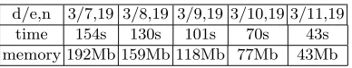
What is interesting is that the time for computing immunity against fast algebraic attacks is almost the same as the one for normal algebraic attacks (see Table 3). There is only little influence of the degreee (see Table 4) on the performance because the size ofQdepends on it. But the time and memory will always stay within a factor two compared to the case whereeis equal ton/2.
d/e,n 2/8,17 3/8,17 3/9,19 3/10,21 4/8,17 5/8,17 6/8,17 D 154 834 1160 1562 3214 9402 21778 time 1s 15s 101s 614s 82s 297s 801s memory 14Mb 25Mb 118Mb 547Mb 33Mb 40Mb 45Mb
Table 3.time and memory for computing the immunity against fast algebraic attacks using Wiedemann’s algorithm. Here we chosen= 2e+ 1.
d/e,n 3/7,19 3/8,19 3/9,19 3/10,19 3/11,19 time 154s 130s 101s 70s 43s memory 192Mb 159Mb 118Mb 77Mb 43Mb
Table 4.dependence of fast algebraic attacks immunity computation in the parameter
e. In all cases.
5
Conclusion
- It is easy to understand since it is based on a well known sparse linear algebra algorithm.
- Its complexity is quite good, especially for the fast algebraic attacks.
- It uses little memory compared to the other known algorithms which make it able to deal with more variables.
- And it is quite general since it can work for both attacks with little modifi-cation. In particular, if in the future one is interested in other kind of relations defined point by point, then the same approach can be used.
Acknoweldegement
I want to thank Jean-Pierre Tillich for his great help in writting this paper and Yann Laigle-Chapuy for his efficient implementation of the fast binary Mo¨ebius transform in SSE2.
References
[ACG+06] Frederik Armknetcht, Claude Carlet, Philippe Gaborit, Simon K¨unzli, Willi
Meier, and Olivier Ruatta. Efficient computation of algebraic immunity for algebraic and fast algebraic attacks. EUROCRYPT 2006, 2006.
[Arm04] Frederick Armknetch. Improving fast algebraic attacks. In Fast Software Encryption, FSE, volume 3017 ofLNCS, pages 65–82. Springer Verlag, 2004. http://eprint.iacr.org/2004/185/.
[BLP06] An Braeken, Joseph Lano, and Bart Preneel. Evaluating the resistance of stream ciphers with lenear feedback agasint fast algebraic attacks. To appears in ACISP 06, 2006.
[BP05] An Braeken and Bart Preneel. On the algebraic immunity of symmetric Boolean functions. 2005. http://eprint.iacr.org/2005/245/.
[Car04] Claude Carlet. Improving the algebraic immunity of resilient and nonlinear functions and constructing bent functions. 2004. http://eprint.iacr.org/2004/276/.
[CM03] Nicolas Courtois and Willi Meier. Algebraic attacks on stream ciphers with linear feedback. Advances in Cryptology – EUROCRYPT 2003, LNCS 2656:346–359, 2003.
[Cop94] Don Coppersmith. Solving linear equations over GF(2) via block Wiede-mann algorithm. Math. Comp., 62(205):333–350, January 1994.
[COS86] D. Coppersmith, A. Odlyzko, and R. Schroeppel. Discrete logarithms in GF(p). Algorithmitica, 1:1–15, 1986.
[Cou03] Nicolas Courtois. Fast algebraic attacks on stream ciphers with linear feed-back. In Advances in Cryptology-CRYPTO 2003, volume 2729 of LNCS, pages 176–194. Springer Verlag, 2003.
[DGM04] Deepak Kumar Dalai, Kishan Chand Gupta, and Subhamoy Maitra. Results on algebraic immunity for cryptographically significant Boolean functions. InINDOCRYPT, volume 3348 ofLNCS, pages 92–106. Springer, 2004. [DM06] Deepak Kumar Dalai and Subhamoy Maitra. Reducing the number of
[DMS05] Deepak Kumar Dalai, Subhamoy Maitra, and Sumanta Sarkar. Basic theory in construction of Boolean functions with maximum possible annihilator immunity. 2005. http://eprint.iacr.org/2005/229/.
[DT06] Fr´ed´eric Didier and Jean-Pierre Tillich. Computing the algebraic immunity efficiently. Fast Software Encryption, FSE, 2006.
[FA03] J.-C. Faug`ere and G. Ars. An algebraic cryptanalysis of nonlinear filter generator using Gr¨obner bases. Rapport de Recherche INRIA, 4739, 2003. [HR04] P. Hawkes and G. C. Rose. Rewriting varaibles: The complexity of fast
algebraic attacks on stream ciphers. In Advances in Cryptology-CRYPTO 2004, volume 3152 ofLNCS, pages 390–406. Springer Verlag, 2004. [Mas69] J. L. Massey. Shift-register synthesis and BCH decoding. IEEE Trans. Inf.
Theory, IT-15:122–127, 1969.
[MPC04] Willi Meier, Enes Pasalic, and Claude Carlet. Algebraic attacks and decom-position of Boolean functions. LNCS, 3027:474–491, April 2004.
[Odl84] Andrew M. Odlyzko. Discrete logarithms in finite fields and their cryp-tographic significance. In Theory and Application of Cryptographic Tech-niques, pages 224–314, 1984.
[Wie86] Douglas H. Wiedemann. Solving sparse linear equations over finite fields.