Unified model for the heat transfer processes that occur during canning, SSHE and electrical resistance aseptic processing of food products that contain large particles

PROCESsES THAT OCCUR DUlliNG CANNING, SSHE AND ELECTRlCAL RESISTANCE ASEPTIC PROCESSING OF FOOD PRODUCTS THAT CONTAIN LARGE PARTICLES

by

JoSeF. Pastrana, HarveyJ.Gold and Kenneth R. Swanzel

Institute ofStatistial

Mm.""

Serial #2230 BMA Series

#

36

MIMED

Pastrana, Gold

&

SERIES

Swartzel

2230

UNIFIED MODEL FOR THE

HEAT TRANSFER PROCESSES THAT

~

OCCUR DURING CANNING, SSHE

&

ELECTIRCAL RESISTANCE ASEPTIC

OF FOOT PRODUCTS •..

..

•

UNIFIED MODEL FOR THE HEAT TRANSFER PROCESSES THAT OCCUR DURING CANNING, SSHE AND ELECTRICAL RESISTANCE ASEPTIC PROCESSING OF FOOD PRODUCTS THAT CONTAIN LARGE PARTICLES*

by

Jose F. Pastrana, HarveyJ. Gold and Kenneth R. Swartzel

*

Paper No. 2230 in the Institute of Statistics Mimeo Series, and No.36 in the Biomathematics !

Series. Department of Statistics, Biomathematics Graduate Program, North Car6lina State University, Raleigh, NC27695-8203

•

ABSTRACT

A unified general model for the heat transfer processes that occur within a food product subjected to canning or aseptic thermal treatment, is presented. Two principles are extensively used in the model building process: system segregation and energy balancing. The model is summarized in an algorithm, whose specification is showed for different combinations of processing system type (PST) and product formulation (PF) with a single particle type. A discussion on the practical relevance of proper product identification in the case of aseptic processing, is included. Finally, an illustration is given on the results that can be obtained from the model algorithm application, in a comparative study of different PST-PF combinations.

INTRODUCTION

A

food product may be thermally treated by pasteurization, conventional canning or aseptic processing. The purpose of aseptic processing is to endow the food product with

,

commercial sterility, a condition in which the product is free of viable microorganisms with

I

either public health significance, as well as those of non-health significance, capable of reproducing under normal non-refrigerated conditions of storage and distribution (FPI, 1989). When a food product is subjected to a thermal !!eatment, there are heat transfer processes that take place. The driving force of such processes is the temperature gradients within the product. This paper describes a model of th_e heat transfer processes in thermal treatment of a food product consisting of a fluid medium with large particles. An example would be beef stew. The model is general enough to describe aseptic processing as well as conventional canning. It

is intended to be used for simulating aseptic processing, as a guide for making decisions

relating to the design of aseptic processing equipment and as the basis for estimating the sensitivity of the degree of sterilization and of the quality degradation to errors in process control, to variation in product formulation and to variability of the physical characteristics of the food material. An important feature of the model is its ability to estimate temperature at the slowest heating locations, which is difficult or impossible to measure with current techniques.

In developing the model, the system structure is represented by defining relevant components, and by defining the input-output relations (exchanges of energy) between the components, as well as the inputs and outputs for the overall system. Processes modeled within the components include fluid flow, heat diffusion within fluid and particulate phases, heat transfer between the phases and, for electrical resistance (ER) heating, conversion of electrical to heat energy (for discussions on the modeling approach, see Gold, 1985, Zeigler, 1976). In a subsequent paper, we will report on the structure of a computer program based on the model discussed here (Pastrana et. aI, 1992b).

The modeling of the heat transfer processes that take place when a thermal treatment is applied to a particulate-laden food product was pioneered by de Ruyter and Brunet (1973) and by Mason and Cullen (1974). Sastry (1986) made a substantial contribution: in this area, and Sastry (1988) presented an overview of modeling approaches and problems encountered. Sastry (1986, 1988) introduced the idea of using energy balances over incremental volumes in a heater (H), which consisted in a scraped surface heat exchanger (SSHE), and a holding tube or thermoequilibrator (THEQ), to obtain fluid medium temperatures. The same idea of energy balances to obtain fluid temperature was later applied, and extended to the cooler (C), by Chandarana and Gavin (1989a), Chandarana et. al (1989b), and Larkin (1990). Instead of using incremental energy balances to obtain carrier medium temperatures, some authors have applied average temperature profiles for the fluid, computed according to different equations:

Larkin et. al (1989), Armenante et. al (1990) and Lee et. al (1990). In constructing the model presented in this paper, extensive use was made of the idea of local energy balances:

A solid particle as a subsystem, is first considered as the union of mutually exclusive and exhaustive regions, then energy balances are established for each region to arrive at a system of ordinary differential equations (ODE), which describes the heat transfer by conduction taking place within the solid particle.

Since some of the equations in the ODE system (those that correspond to the solid particle surface) depend on the surrounding fluid temperature, there is a need to know or estimate that temperature. This may be done in three alternative ways: by direct measurement (although the most accurate, it requires that the system be physically constructed), by fluid energy balances on incremental volumes in the system equipment (Sastry, 1986; Chandarana and Gavin, 1989a; Chandarana et. aI, 1989b; Larkin, 1990), and by assuming an average fluid temperature profile (Larkin, 1989; Armenante et. aI, 1990; Lee et. aI, 1990). In our model, we use the local energy balance principle following Sastry (1986), to obtain an estima.te of the fluid temperature profile as the product flows through the system. We make the simplifying assumptions that the fluid is well mixed (in the radial direction for aseptic proc~ingand in all directions for canning), and that there is piston (plug) flow throughout.

The model proposed in this paper differs from Sastry's (1986), in several respects: In addition to the SSHE system, it includes elec~ical resistance aseptic and canning processing,

and also adds the cooling stage.

It applies mean interstitial fluid velocity, as a normalizing constant in the thermoequilibrator velocity ratio (THEQVR) (Barry, 1991). A mean bulk product velocity is implied when mean bulk residence time is used as normalizing constant in the residence time ratio (RTR).

,

A target for the fastest heating zone (FHZ) temperature at heater exit (y~,j)' is established as in Chandarana and Gavin (1989a), Chandarana et. al (1989b), Larkin (1989,1990) and Lee et. al (1990).

A target for the fluid temperature at system exit (y~,/), is established. A similar target for the warmest zone proved to be too strong a requirement for a particular product formulation (PF), under ER aseptic processing (Pastrana et. all, 1992b)

Irregular shapes are not considered for the solid particles, since any irregular shape can be included in an appropriate imaginary regular shape, such as a sphere or parallelepiped.

A subsequent paper (Pastrana et. all, 1992b) will report on the applications of the model to specific PF (beef in gravy without starch, and beef in gravy with starch having equal or greater electrical conductivity than the beef).

THEORY

SYSTEM DEFINITION AND STRUCTURE

We are concerned with modeling changes in a food product, which consists of particles in a fluid medium. The relevant changes which are induced by the thermal treatment (canning, ER or SSHE aseptic thermal treatment) include microbial and spore load, enzyme concentration, nutrient retention and other measures of food quality. The thermal treatment consists of the following stages (shown with abbreviations which will be used): heating (H), thermoequilibrium (THEQ), and cooling (C). The H stage consists in the application of a heat source by means of pressurized steam (canning and SSHE aseptic processing) or an electrical current( ER aseptic processing). The product temperature at any point is expected to increase during the H stage. The THEQ stage follows immediately the H stage and consists of a holding stage during which the product is expected to reach thermal equilibrium, in which thermal gradients would disappear. The C stage follows immediately the THEQ stage. It consists of . applying a heat sink by means of cooling water, so that the produ"ct temperature at any point

is expected to decrease.

The thermal state of the system at any given time is specified by the product temperature distribution. The devices associated with each stage for the different types of thermal treatment are as follows:

DEVICE STAGE

H

THEQ

C

Canning Rotating retort at temperature below retort temperature (RT) and under pressurized steam. Rotating retort at temperature equal to RT, and under pressu rized steam.

Rotating retort under cooling water.

Aseptic SSHE or ER heater.

Stainless steel insulated tube.

FIG.1 shows a flowchart of the general system:

DEVICE 1 DEVICE 2 DEVICE 3

I

H stage

1 - - - -

1

I

_{THEQ stage}

1---1

_{C stage}

I

time FIG. 1: Flowchart of the general system

SYSTEM INPUTS, OUTPUTS AND ENVIRONMENT

The input to the system is energy. For canning or SSHE aseptic processing, the main input energy is in the form of heat transfer from a heating medium. For ER aseptic processing, the main input energy is in the form of electrical energy delivered by subjecting the product to an alternating electrical current.The output from the system is energy. The main output energy is the form of heat transfer to the cooling medium.The environment is considered to be everything apart from the system that may transfer heat to, or receive heat from, the: system. In particular, the environment includes the supporting systems needed to preheat the product, raise the heating medium temperature and lower the cooling medium temperature.

SYSTEM COMPONENTS, THEIR INPUTS AND OUTPUTS Component

1

It includes DEVICE 1 (FIG. 1) plus the particulate-laden product being heated. The input is the same as the system energy input and the output is heat transferred to component 2 through a heated product.

Component

2

It includes DEVICE 2 plus the heated particulate-laden product being already in thermoequilibrium. The input is the same as the output from component 1 and the output is heat transferred to component3 in the form of a food product in thermoequilibrium.

Component

a

It includes DEVICE 3 plus the particulate-laden product in thermoequilibrium being cooled. The input is equal to the output from component 2and the output coincides with the system energy output.

The heating stage for canning and SSHE aseptic processing involves convective and conductive heat transfer processes as follows:

convective PARTICLE conductive PARTICLE

SURFACE CENTER

T

T

T convection product-interior wall;

T conduction through wall; convective at steam-external wall T

HEATING MEDIUM

FIG. 2: Heat transfer during canning and SSHE H stage

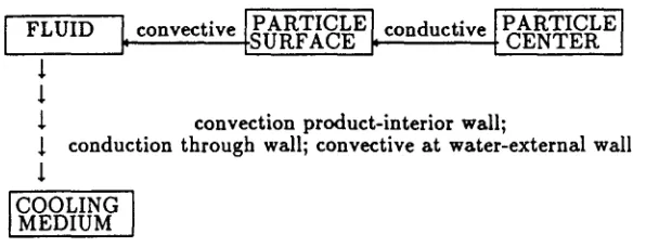
convective PARTICLE conductive PARTICLE

SURFACE CENTER

1

1

1

convection product-interior wall;

1

conduction through wall; convective at water-external wall

1

COOLING MEDIUM

FIG. 3: Heat transfer during canning SSHE C stage

When the fluid is the FHZ during ER heating, the fluid and particle surface are also heat donors as for SSHE heating (FIG. 1), except that in that case the heating medium is the product itself.

FIG. 4 shows the convective and conductive heat transfer processes for the THEQ stage; the arrows go from fluid to ambient for aseptic processing, and from constant steam temperature to fluid for canning:

convective PARTICLE conductive PARTICLE

SURFACE CENTER

II

II

II

convection product-interior wall;

1

r

conduction through wall; convective at surroundings-external wall

H

AMBIENT OR CaNST. TEMP. STEAM

FIG. 4: Heat transfer during THEQ stage

i ,

;-MODEL BUILDING PROCESS Introduction

The model is designed to yield estimates, at any point in the processing system, of variables which depend upon temperature history of the food product. Some important variables which we consider are:

Nutritional quality variables:

Nutrient percent concentration.

Point or integrated nutrient equivalent thermal destruction times. Sterility variables:

Spores percent concentration.

Point or integrated spore equivalent thermal destruction times. Chemical variables:

Enzyme percent concentration

Point or integrated enzyme equivalent thermal destruction time

As already described, the system consists of a particulate-laden food product subject to a thermal treatment that comprises three stages, each ~tagecarried out in a particular DEVICE. In canning, a specific food product volume is well identified because it is contained in a hermetically closed container ( a 211 x 214 tin plate can). However, for SSHE aseptic and ER

--"

aseptic processing, the volume of food product, whose state and quality are of concern, is not well identified, since volume elements mix with each other as the food travels through the equipment. However, when the main interest centers on determining the fastest solid particle thermal state ( that is, its temperature), then the food product volume identification is not a serious problem, as long as two conditions hold: first, the solid particle considered for modeling

purposes is the one that contains the product's slowest heating zone (5HZ) , and second, the surrounding fluid temperature is known. As indicated in the INTRODUCTION of this paper, three ways to generate a carrier fluid temperature profile are: by direct measurement; by computation of fluid energy balances, and by assuming an average temperature profile. The second, which is the one followed in this paper, idealizes, for the purpose of generating a carrier fluid temperature profile, the existence of a thermodynamic control volume (Van Wylen and Sonntag, 1985). The coordinate system that allows the volume localization is a translating system along the horizontal axis (imaginary incremental volumel , assumed to move horizontally in a horizontal processing system).

Although the control volume contains, at a given instant, a thermally treated product, it is true that the product is still not well identified, since mass gets in and out the control volume. Should plug (piston) flow hold throughout for aseptic processing, then the problem of control-volume product identification would disappear.

Modeling assumptions

The following assumptions are made in order to simplify the model:

a) All solid particles are identical with respect to size , shape, and other relevant I

characteristics.

b) The product fluid in the reference volume is well mixed, so that fluid temperature is uniform.

c) For canning, the resistance to heat transfer offered by the metal can wall, is ignored.

d) For aseptic processing, H stage exit FHZ temperature and C stage (system) exit fluid temperature equal to their targets, as indicated in the INTRODUCTION, and are set by

lThe volume of a 211 x 214 tin plate can, and of the hypothetical incremental volume are here on referred to as "reference volume".

..

the operator. For canning, constant pressurized steam and cooling water temperatures, were fixed; although the same fluid exit temperature target was required as for aseptic processing, no corresponding target was set, at the H stage exit.

e) Initial temperature distribution within the reference volume is uniform and equal to a constant YIat every point in the product.

f) For aseptic processing, a particular configuration is assumed where devices are straight, lined up horizontally, directly connected one after the other, and with no bends.

g) For ER heating, the following specific assumptions are made: all electrical energy IS

converted into thermal energy; the effect on temperature of the particle orientation relative to the electrical field lines is negligible (reasonable for cubic shapes); the ratio between the solid and fluid electrical conductivities is invariant with temperature. h) Applicable hfp is the same for canning as for aseptic processing.

Basic modeling principles

Two basic principles have been applied in the modeling building process. These are i

appropriate segregation of the system, and thermodynamic modeling of local energy balances._, Appropriate segregation of the system:

First, the system is divided into three components,' as indicated in the section SYSTEM COMPONENTS, THEIR INPUTS AND OUTPUTS.

Second, within each component, one of the identical (see assumption a)) solid particles

isconsidered. In aseptic processing, the particle considered is the fastest moving particle. Third, a volume of product containing this particle is considered.

The segregation is carried further by segregating the food particle, into mutually exclusive and exhaustive regions, where each region within the solid particle is

,

considered to be a thermodynamic subsystem (a partition of the solid particle that is suitable for numerical integration, is convenient here). The volume of product that contains the fastest moving solid particle, is also segregated into two thermodynamic subsystems: the fluid phase and the solid phase; the latter consists of the solid particles (beef cubes), each being partitioned identically.

Local energy balances:

An energy balance is an equality between the sum of the rates of energy inputs (sources), and the sum of the rates of energy uses. It is a generalization of the work-energy theorem of mechanics, which sometimes is referred to as the general form of the first law of Thermodynamics (Sears and Salinger, 1986).

Possible energy sources are:

Energy input (E_{in )} such as heat transfer input and energy generated (E_g) by the system

resistance to an electrical current. Possible energy uses are:

Energy output (E_{out )} such as heat transfer output and thermal energy (E,) stored in the form of internal energy.

An energy balance takes the form(Myers, 1976):

•

•

•

•

Ein

+

Eg= Eout

+

E.

For a thermodynamic subsystem during canning or SSHE aseptic processing:

•

•

•

Ein

=

Eout

+

E. since there is no heat generation in such cases (no electric current is applied, as during ER heating).

During ER heating:

•

•

•

E9

=

Eout

+

E. since there is no heat transfer applied in such case.

Following Myers (1976), the different rates in the energy balance equation are given

by:

•

E -_{g -} g"'V

• 8y

E.

=

_pVr8t

Model algorithms to obtain reference volume temperature spatial distribution

The following algorithm allows the estimation of the temperature distribution in the reference volume for canning and, under the assumption that THEQVR=l, for aseptic processing. For the first algorithm iteration, t_i is set equal to 0:

a) Consider the product in the reference volume to be subjected to a thermodynamic process that consists of heating (if product is in DEVICE 1), thermoequilibrium (if product is in DEVICE 2), or cooling (if product is in DEVICE 3) from time t_i to time t_{e ,}

te=t_i

+

6t, where 6t is a time increment (also called variable time step). Assume plug flow for aseptic processing.

b) Partition each food particle in the reference volume identically i:nto disjoint and exhaustive regions, and consider each region within the food particle to be a thermodynamic subsystem.

c) Establish energy balances for each region included in the food pa~ticle, and express them as a system of ordinary differential equations (ODE's). Since the energy balances for the regions of the food particle that contain a portion of the particle surface, depend onYf'

there is one more unknown than equations, so that an additional ODE is needed, or one of the variables (fluid or local regions temperature) must be known, in order to solve the system of ODE's.

d) Obtain the needed extra ODE (see c) above), by performing an energy balance on the reference volume fluid.

e) Solve the system of ODE's, storing 'IIf in a vector of fluid temperatures 'III for the aseptic processing ease, so that the fastest particle surrounding fluid temperature can be computed later. These stored fluid temperatures will be referred to as plug flow fluid temperatures. In the numerical integration, a variable time step method that uses 4th and 5th order Runge Kutta schemes maybe applied (Pastrana et. ai, 1992c). At time tout this gives an estimate of the spatial temperature distribution.

f) Set tj = t_e

,

and take last temperature estimates as initial estimates.

g) Repeat the whole process until t_e becomes equal to the processing system exit time.

For aseptic processing, the temperature spatial distribution of the fastest food particle is computed by applying the following algorithm, first setting tj = 0:

a) Consider the product enclosed in a reference volume Qx

at

that contains the fastest particle, where Q is the volumetric flow rate, and a thermodynamic process (heating, thermoequilibrium or cooling) from tjto t_e, te=tj+at, on that product.

b) Partition the fastest food particle into disjoint and exhaustive regions, and consider each region included in the food particle tobe a thermodynamic subsystem.

c) Establish energy balances for each of the regions of the fastest particle, expressing them as a system of ODE's.

d) Find the temperature of the fluid surrounding the fastest particle by applying the stored plug flow fluid temperature profile:

fastest particle position= particle velocity x tj particle position plug flow fluid corresponding time

fluid velocity

. __ . _ l .•

•

.

#

The surrounding fluid for the fastest particle, has a temperature approximately equal to the stored plug flow fluid temperature that corresponds to the above plug flow fluid time (entry in 11/ associated to time less or equal to such plug flow time).

e) Solve the system of ODE's applying the surrounding fluid temperature obtained in the previouS step. At time t_e this gives an estimate of the spatial temperature distribution of the product enclosed in the reference volume containing the fastest particle.

f) Set t_i

=

t_e and take the last temperature estimates as initial estimates. g) Repeat the whole process until t_e is equal to the processing system exit time.

Residence time considerations in aseptic processing

The stored plug flow fluid temperatures allow the computation of the temperature distribution for the fastest particle, under various assumptions concerning residence time at high product flow rates:

a) Plug flow in each device. This could be a reasonable scenario when the product flow is turbulent throughout.

b) Plug flow in the H and the C stages, but bimodal normally distributed residence time ratio

i

(RTR) in the THEQ. This scenario may be appropriate when the flow is turbulent in

i

the Hand C. There is experimental evidence, such as with the PF's considered by us, that the RTR distribution is likely to be bimodal normal in the THEQ (Berry, 1989; Dutta and Sastry, 1990; Palmieri, 1991). This is the residence time scenario 5ltosen for the model applications (Pastrana et. aI, 1992b).

Taeymans et. al, 1985). As pointed out in b) immediately above, there is experimental evidence that suggests the possibility of a bimodal normal RTR in the THEQ, for the PF's considered by us. This scenario may be modified by assuming plug flow in the THEQ, when the flow there, is turbulent.

d) Plug flow in the electrical resistance (ER) heater, and THEQ, and exponentially distributed RTR in the C. This residence time scenario may be appropriate when there is turbulent flow in the ER heater and THEQ, and there is mixing in the radial and axial direction in the C.

Model equations

The model equations consist of a system of ODE's derived from the energy balances performed according to the algorithms described previously. The specific form of the equations depend on several factors:

Particle shape. This may be regular (spherical, cubic, etc.) or irregular.

Manner in which the particie is segregated into regions. The type of segregation depends on the particle shape, and presupposes a strategy to solve the system of ODE's (finite difference, finite element, etc.).

Region location within the particle. The region location is described by the corresponding node location: in the interior, at the boundary and/or surface. In the case of the cubic shape, considered in the model applications (Pastrana et. al, 1992b, 1992c, 1992d), surface regions correspond to: non-edge, edge but not at the corner, and corner nodes. Thermal treatment stage. The heat transfer processes change, and there are different pertinent

parameters in each stage.

The system of ODE's shown below is for the H stage of a product that consists of cubic particles (beef cubes) in a fluid (gravy with or without starch). Under the assumption of

..

uniform fluid temperature, there is symmetry in the convective heat transfer from (to) the fluid to (from) the particle faces, which allows consideration of just one octant of the cube in setting the system of ODE's. The cube octant was segregated into small volume units or regions, by applying the finite difference method (Myers, 1971).

To illustrate, when the octant edge is divided into 3 congruent segments, the number of discrete points on the octant edge (n) is 4: two endpoints and two interior points. Letting (ij,k) represent an arbitrary point in the resulting octant grid, ij,k=I,2,3 or 4, there are 64 points (ij,k), called nodes, each of which can be monitored as far as spore, enzyme, and nutrient thermal destruction. The idea is to assign an octant volume unit, that is, an octant region, to each node, and assume uniform thermal conditions for the octant region. Following Myers's nodal point arrangement (Myers, 1971), octant regions are assigned to the nodes so that any octant cross section, yields regions in two dimensions, as described in FIG. 5A. The regions assigned to nodes (1,1,1), and (n,n,n) (lower left and upper right regions in FIG. 5B) are of particular interest in the applications, because one of them corresponds to the fastest beef cube 5HZ, while the other to the 5HZ (See ILLUSTRATION Section in this paper, and Pastrana et. ai, 1992b and d).

I The volume of a region assigned to a node included in any face of the cube oct~nt, is just a fraction of the common volume of an interior· (non-face) region:

1

if node is at the face corner, ~ if node is at the face edge but is not in the corner, and! if node is in the face but not at the edge. This fact was carefully considered when establishing the energy balance otany region assigned to a node in the face of the cube octant.

,

There are six faces in a beef cube octant; three of them have direct contact with the fluid, and the other three, have direct contact with neighboring octant cubes. Regions in any of the former three faces, correspond to nodes (ij,k) with at least one of i,j and k equal to 1; the energy balances for these regions must include a convective boundary condition. Regions in any of the latter three faces, correspond to nodes (ij,k) with at least one of i, j and k equal to nj the energy balances for these regions include a symmetric boundary condition.

.,

_,

, i !

- ,i l '

;r)

H

,c. ' I

I II ~! I

!

I

I

_I r--;i

'3

u

I " , II '__Ii

!

i I i 1 ! I I I

!

i

!

.L.---L---+---r--~i

!

,

i

!

I

I

! ! I , I !

i

i

I

I

i

1

L

1

---~---;----___:---;---___1---___j

I 1 , " r ----' ,..----,

11

!

I ' I

, ,

'--'

12

!

I I

-'-r - - ;

lA-I

I . "

y

FIG. SA: Two dimensional regions obtained by any cross section of the cube octant.

Axis identification is as follows, assuming that the cube is centered at the origin, and its sides lie on the coordinate system axes:

k'lXYXxY\~'X!·I··i":··:·':':Ei!iiE!!iiE:5ii;~~~~

VX':xY6Yx~U\~i£'

"", '

!<:Xx:\!.X\i\!i,·

'»:oj>.

l;,..., ....~..AJA..·I\··\i··/·

.... (11

A)1

~\Ioae " I"

!

! ,

FIG. 58: Regions within the cube octant that correspond to nodes (1,1,1) and (n,n,n). Each octant side is partitioned into 3 congruent segments, so that there are n=4 nodes on each octant edge.

..

The energy balances for the fluid and regions within a particle, established according to the above algorithms steps, include when applicable, the rate of thermal energy generated, the rate of heat transferred by convection to or from the fluid, the rate of heat transferred by conduction to or from neighboring particle regions, and the rate of energy stored in the form of internal energy.· As an example, the fluid energy balance includes the following energy sources and uses:

Sources:

Thermal energy generated (as in the ER).

Heat transferred by convection from a heating medium (as in canning, SSHE, and depending on PF, in ER processing).

Uses:

Energy stored in the form of internal energy.

Energy transferred by convection to the particles (as in canning and SSHE and, depending on PF, in ER processing).

The equations that appear below were derived by Jose Pastrana. In them, vs=O for

the canning H stage and SSHE aseptic processing (since no electrical current is applied),

, Uh

=

0 for ER heating (there is no heat transfer through the ER wall), and the parameters

m6t' A_{6t ,} N6t' V6t' and Y.t depend on the processing system considered. Derivative of fluid temperature

OYf 2 _

Tt=1.0j(m6tx"Yf)x (UhxA_6tx_(Y.CYf)-hfpx24.0xI xN6tx(YrY )+

«V6t1(A_erXL_er»2)xVBX(Tf X(1.0+6fey r25.O» X€ X(A_er2)jV6t)

In the case of SSHE and ER aseptic processing, this derivative depends on the time step

ot,

since the volume of fluid (included in the reference volume product), depends on

ot.

The necessary steps to obtain this equation are presented in an APPENDIX at the end of this Manuscript.

Derivatives of cube octant temperatures a) At octant interior nodes:

1t<ij,k)=(a/e52) x (y(i-1j,k)-6.0 x y(ij,k) + y(i+1j,k)+

y(ij-1,k) + y(ij+1,k) + y(ij,k-1) + y(ij,k+1)+

«15/L_er)2)xvsX0"Px (l.O+m_px (y(ij,k)-25.0))/k_{p }} ij,k=2, n-1

b) At nodes in the three cube octant faces that have direct contact with the fluid. A convective boundary condition was considered when establishing the corresponding energy balances.

bl) Nodes not at the edges:

1t<lj,k)=(a/62)x(2.0xBix(Yry(lj,k))+

y(lj-I,k)-6.0 x y(1j,k) + y(1j+1,k) + y(lj,k-1) + y(1j,k+1)+2.0 x y(2j,k)+

4.0x «6/(2.0 xL_er))2)xvsx0"Px (l.O+m_px (y(lj,k) -25.0))/k_p} j,k=2, n-1

~~(ij,1)=(a/62)

x (2.0 x Bi x(Yr y(ij,1))+

y(i-1j,1)-6.0 x y(ij,1) + y(i+1j,1) + y(ij-1,1) + y(ij+1,1)+2.0 x y(ij,2)+

«6/L_er)2)xvsxO"p x (l.O+m_px (y(ij,1)-25.0))/k_p} ij=2, n-1

~~(i,1,k)=(a/62)

x (2.0 x Bi x (y r y(i,1,k)) +

y(i-1,1,k)-6.0 x y(i,1,k) + y(i+1,1,k) + y(i,I,k-1) + y(i,1,k+1)+2.0 x y(i,2,k)+

«6/ L

_er)2) xvsX0"Px (l.O+m_px(y(i,I,k)-25.0))/k_{p }} i,k=2, n-1

b2) Nodes at edges, but not in the corners. A symmetric boundary condition was considered, in addition to the convective one, when establishing the energy balances for the regions assigned to those nodes included also in any of the faces that have direct contact with neighboring octant cubes. The symmetry boundary condition was applied by imposing equalities such as:

..

Derivatives of cube octant temperatures a) At octant interior nodes:

~iJ,k)=(a/52)

x (y(i-lJ,k)-6.0 x y(iJ,k) + y(i+lJ,k)+ y(iJ-l,k) + y(iJ+l,k) + y(iJ,k-l) + y(iJ,k+l)+

«5/L

er)2)xVBX(TPx(l.O+m

p

x(y(iJ,k)-25.0))/k

pp

iJ,k=2, n-I

b) At nodes in the three cube octant faces that have direct contact with the fluid. A convective boundary condition was considered when establishing the corresponding energy balances.

bl) Nodes not at the edges:

~~(IJ,k)=(a/52)

x(2.0xBix(Yry(IJ,k)) +

y(IJ-I,k)-6.0 x y(lj,k) + y(IJ+I,k) + y(lj,k-I) + y(lj,k+I)+2.0 x y(2j,k)+

4.0x «5/(2.0 xL_er))2) xvsx(Tpx (l.O+m_px (y(IJ,k) -25.0))/k

pp

j,k=2, n-I

~~

(iJ,1 )=(a/52)x (2.0 xBix(yry(iJ,I)) +

y(i-IJ,I)-6.0

x

y(iJ,I) + y(i+IJ,I) + y(iJ-I,I) + y(iJ+I,I)+2.0

x

y(iJ,2)+

«5/L

_er)2)xvsX(Tpx (l.O+m_px (y(iJ,I)-25.0))/k_p

p

iJ=2, n-l

~i,I,k)=(a/52)

x (2.0 xBix(yry(i,I,k)) +

y(i-I,I,k)-6.0 x y(i,I,k) + y(i+I,I,k) + y(i,I,k-l) + y(i,I,k+I)+2.0 x y(i,2,k)+

«5/L

er)2)xvsX(TPx (l.O+m_px (y(i,I,k)-25.0))/k_p

p

i,k=2, n-I

b2) Nodes at edges, but not in the corners. A symmetric boundary condition was considered, in addition to the convective one, when establishing the energy balances for the regions assigned to those nodes included also in any of the faces that have direct contact with neighboring octant cubes. The symmetry boundary condition was applied by imposing equalities such as:

'..

y(1,n,k)=y(1,n+1,k) and y(i,1,n)=y(i,1,n+1).

~1,1,k)=(a/62)

x (4.0 x Bi x(Yry(1,1,k))+2.0x y(1,2,k)-6.0 x y(1,1,k) + y(1,1,k-1) + y(1,1,k+1)+2.0 x y(2,1,k)+

4.0 x «6/(2.0 xL_er)?)xVB X0"Px (l.O+m

p

x(y(1,1,k)-25.0))/k

pp

k=2, n-1

~1,n,k)=(a/62)

x (2.0 xBix(y

r

y(1,n,k))+

4.0 x y(1,n-1,k)-8.0 x y(l,n,k) + y(1,n,k-1) + y(1,n,k+l)+2.0 xy(2,n,k)+ 4.0 x «6/(2.0 xL_er))2) xVBX0"P X(l.O+m

p

x (y(1,n,k)-25.0))/k

pp

k=2, n-1

~~(1j,1)=(a/62)

x (4.0 x Bi x (Yry(lj,1))+2.0 x y(1j,2)-6.0 x y(1j,1) + y(1j-1,1) + y(lj+1,1)+2.0 x y(2j,1)+

4.0 x «6/(2.0 xL_er))2)xVBX0"P X(l.O+m_px(y(1j,1)-25.0))/k

pp

j=2, n-1

~~(1j,n)=(a/62)

x (2.0 x Bi x(Yry(lj,n))+4.0 x

y(1j,n-1)-8.0 x y(1j,n) + y(lj-1,n) + y(lj+l,n)+2.0 x y(2j,n)+

4.0 x «6/(2.0 xL_er))2)xVBX0"Px (l.O+m

p

x (y(1j,n)-25.0))/k

pp

j=2, n-1

~~(i,1,1)=(a/62)

x (4.0 x Bi x(y

r y

(i,1,1))+2.0 x

y(i,2,1)-6.0 x y(i,1,1) + y(i-1,1,1) + y(i+l,1,1)+2.0 x y(i,1,2)+

«6/ L

_er)2)xVBX0"P X(l.O+m

p

x (y(k,1,1)-25.0))/k

pp

i=2, n-1

~i,n,1)=(a/62)

x (2.0 x Bi x(y

r

y(i,n,1))+2.0 x y(i,n,2)-8.0 x y(i,n,1)+4.0 x y(i,n-1,1) + y(i-1,n,1) + y(i+1,n,1)+

«6/ L

er)2)xVB X0"P X(l.O+m

p

x (y(k,nn,1)-25.0))/k

pp

i=2, n-1

c) At nodes in the three octant faces that have direct contact with neighboring cube octants. A symmetric boundary condition was considered when establishing the corresponding energy balances. The symmetric boundary condition was applied by imposing equalities such as:

y(n,1,k)=y(n+1,1,k) and y(n,n,k)=y(n,n+1,k).

c1) Nodes not at the edges.

~~(nj,k)=(a/62)

x (y(nj-1,k)-8.0 x y(nj,k)+

y(nj+1,k) + y(nj,k-l) + y(nj,k+1)+4.0 x y(n-lj,k)+

4.0 x ((6/(2.0 xL_er))2) x vs x(jpx (l.O+m_px (y(nj,k)-25.0))/k_{p ),}j,k=2, n-1

~ij,n)=(a/62)

x (4.0 x y(ij,n-l)-8.0 x y(ij,n)+

y(i-1j,n) + y(i+lj,n) + y(ij-l,n) + y(iJ+l,n)+

((6/ L_er)2) x vsX(jPx (l.O+m_px(y(ij,n)-25.0))/k_p).iJ=2, n-1

~~(i,n,k)=(a/62)

x (y(i,n,k-1)-8.0 x y(i,n, k)+

y(i,n,k+l) + y(i-l,n,k) + y(i+l,n,k)+4.0 x y(i,n-l,k)+

((6/ L_er)2) x vs x(jpx (l.O+m_px(y(i,n,k)-25.0))/k_{p ).} i,k=2, n-l

c2) Nodes at the edges, but not in the corners. A convective boundary condition -was considered, in addition to the symmetric one, when establishing the energy balances corresponding to regions assigned to those nodes included also in the faces that have direct contact with the fluid.

,

~~(n,1,k)=(a/62)

x (2.0 x Bi x(y

r y

(n,1,k))+2.0 x

y(n,2,k)-8.0 x y(n,1,k) + y(n,1,k-1) + y(n,1,k+l)+4.0 x y(n-l,l,k)+

4.0 x «6/(2.0 xL_er))2)x vsX(jPx (l.O+m_px (y(n,1,k)-25.0))/k_pp k=2, n-1

~~

(n,n,k)=(a/62) x (4.0 x y(n,n-l,k)-lO.O x y(n,n, k)+ y(n,n,k-l) + y(n,n,k+1)+4.0 x y(n-l,n,k)+

4.0 x «6/(2.0 xL_er))2)x vs x(jpx (l.O+m_px (y(n,n,k)-25.0))/k_{p )'} k=2, n-1

~~(nj,1)=(a/62)

x (2.0 x Bi x (Yry(nj,1))+2.0 x

y(nj,2)-8.0 x y(nj,l) + y(nj-1,1) + y(nj+1,1)+4.0 x y(n-lj,l)+

4 .0 x «6/(2.0 xL_er»2) x vs x(jpx (l.O+m_px (y(nj,1)-25.0))/k_{p ).}j=2, n-l

~~(nj,n)=(a/62)

x (4.0 x y(nj,n-l)-lO.O x y(nj,n)+

y(nj-l,n) + y(nj+l,n)+4.0 x y(n-lj,n)+

4.0 x «6/(2.0 xL_er))2)x vsX(jPx (l.O+m_px (y(nj,n)-25.0))/k_ppj=2, n-l

~~(i,1,n)=(a/62)

x (2.0 x Bi x(y

r y

(i,1,n))+4.0 x y(i,1,n-1)-8.0 x y(i,1,n)+2.0 x y(i,2,n) + y(i-l,l,n) + y(i+l,1,n)+

«6/ L

_er)2) x vsX(jPx (1.0+m_px (y(i,1,n)-25.0))/

k

pp

i=2, n-l

~i,n,n)=(a/62)

x (4.0 x y(i,n,n-l)-lO.O x y(i,n,n)+

(i-l,n,n) + y(i+l,n,n)+4.0 x y(i,n-l,n)+

«6/ L

_er)2) x vsX(jPx (1.0+m_px (y(i,n,n)-25.0))/k_pp i=2, n-1

d) At corner nodes.

~1,1,1)=(2.0

xa/52) X(3.0 x Bi x (Yry(l,l,l» + y(1,2,1)-3.0 x y(l,l,l) + y(1,1,2) + y(2,1,1)+

2.0 x «5/(2.0 xL_er»2)xVB X (TPx (1.0+m_px (y(1,1,1)-25.0»/k_{p )}

~~(1,1,n)=(2.0

xa/52)x (2.0 x Bi x (Yry(l,l,n» +

y(1,2,n)-4.0 x y(1,1,n)+2.0 x y(l,l,n-l) + y(2,1,n)+

2.0 x «5/(2.0 xL_er»2)xVBX(TPx (1.0+m_px (y(1,1,n)-25.0»/k_{p )}

~~(1,n,1)=(2.0

xa/52)x (2.0 x Bi x (yr y(1,n,1»+2.0 x

y(l,n-l,1)-4.0 x y(l,n,l) + y(1,n,2) + y(2,n,1)+

2.0 x «5/(2.0 xL_er»2)xVBX(TPx (1.0+m_px (y(1,n,1)-25.0»/k_{p )}

~1,n,n)=(2.0

xa/52)x (Bi x (y ry(l,n,n»)+

2.0 x y(1,n,n-l)-5.0 x y(l,n,n)+2.0 x y(n,n-l,n) + y(2,n,n)+ 2.0 x «5/(2.0 xL_er»2)xVBX(TPx (1.0+m_px (y(1,n,n)-25.0»/k_{p )}

~n,1,1)=(2.0

xa/52)x (2.0 x Hi x(yry(n,l,l» + y(n,2,1)-4.0 x y(n,l,l) + y(n,1,2)+2.0 x y(n-l,n,l)+

2.0 x «5/(2.0 xL_er»2)xVBX(TPx (1.0+m_p x (y(n,1,1)-25.0»/k_{p )}

~n,1,n)=(2.0

xa/52)x (Hi x (Yry(n,l,n» +

y(n,2,n)-5.0 x y(n,1,n)+2.0 x y(n,1,n-l)+2.0 x y(n-l,l,n)+

2.0 x «6/(2.0 xL_er»2)xVB X (TPx (1.0+m_px (y(n,1,n)-25.0»/k_{p )}

i

.

~n,n,1)=(2.0

xa/52)x (Bi x (Yr y(n,n,1»+

y(n,n,2)-5.0 x y(n,n,1)+2.0 x y(n,n-1,nn)+2.0 x y(n-1,n,1)+

2.0 x «5/(2.0 xL_er»2)x vsXupx (l.O+m_px (y(n,n,l)-25.0»/k_{p )}

~n,n,n)=(2.0

xa/52) x (2.0 x

y(n,n-1,n)-6.0 x y(n,n,n)+2.0 x y(n,n,n-1)+2.0 x y(n-1,n,n)+

2.0 x «5/(2.0 xL_er»2)x vsXupx (l.O+m_p x (y(n,n,n)-25.0»/k_{p )}

Kinetics

As indicated in the Introduction of this section, the model was designed with the goal of obtaining estimates of variables which depend upon the temperature history of the food product. Once an estimate of the temperature spatial distribution is available for the product enclosed in the reference volume (containing the fastest particle in the case of aseptic processing), the evaluation of any temperature dependent variable, is straightforward:

a) Point equivalent thermal destruction time for spores, enzymes and nutrients. The computation is done by applying the General Method of accumulated lethality computation (Pflug, 1990). For spores (of Clostridium Botulinum, say), this method was applied in the time interval from t_i to t_{e for any of the product elements (fluid and} beef cube regions), by obtaining the point equivalent destruction time or kill time (F0) (Pflug, 1990), at the reference temperature (Yo' Yo = 121.1·C). The kill time is equal to the product of the time interval length (t_{e -} t_{i ),} by the lethality rate (L) (ratio of exposure time F0 at the reference temperature yo to exposure timeF at a temperature y

F_{o=(te- t}j ) xL, at the fluid or cube octant region with center node (iJ,k).

When the Bigelow model holds for relative times of thermal destruction (Pflug, 1990):

The accumulated kill time (sterility), for a relatively long time interval is computed by adding the kill times of a partition of subintervals. For constituents such as enzymes (peroxidase for example) or nutrients (thiamine for example), the same procedure is applied to obtain the corresponding equivalent destruction times.

b) Concentration of spores, enzymes and nutrients. The following formula is applied to compute the concentration Ce in any product element at time t_{e ,} given an initial concentrationtp at time tj

=

0:

An alternative way of obtaining Ce is by applying actual tiIJl.e F, instead of kill time

I

F0' but adjusting the D values (Teixeira et al., 1964; Teixeira and Shoemaker, 1989).

The total concentrations are obtained by adding the products C_ex product element volume.

c) Integrated equivalent destruction times Flat time t_e for the product included in the reference volume. The initial concentration tp at time tj

=

0, and the concentration C e

at time t_e must be known in order to apply the following formula (Stumbo, 1965):

ILLUSTRATION

Two alternative PF's of beef in gravy were considered, one without starch, denoted as BBROTH, and other containing 3% crosslinked starch, denoted as STARCH2• The thermal

processing of each PF was simulated for each processing system type (PST): SSHE aseptic (PST=1), ER aseptic (PST=2), and canning (PST=3). A lethality target of 360 seconds (s) at a reference temperature equal to 121.1 ·C, was required for the THEQ stage. The results that appear in FIGURES 6 to 10 were obtained under worst case conditions: minimum convective heat transfer coefficient (h_{Jp )' and for aseptic processing, maximum fastest particle velocity} ratio in the thermoequilibrator (THEQVR=2). The equivalent destruction times shown in the . figures, are given at a reference temperature (Y_{r ),} equal to 121.1 ·C(250 "F).

Although all PST's were required to have the same system exit fluid temperature (32.2·C), a pressurized steam constant temperature was assumed for PST=3 (115.6 .C), and a target fluid temperature (140 ·C) at H exit, was imposed for PST=1 and PST=2. Constant cooling water temperature was also assumed for PST=3 (18.3 ·C). Adjustable pressurized steam and cooling water temperatures were considered for PST=1 and PST=2.

For any of the PST's and PF's considered in this illustration, the fluid is the fastest heating zone (FHZ) of the product included in the reference volume, the octant region assigned to node (1,1,1) is the octant (and whole beef cube) FHZ, and the region assigned to node

(n.n,n), is the octant (particle) slowest heating zone (SHZ) (FIG.6). For a PST and PF combination where the fluid is the SHZ, see Pastrana et. al (1992 b).

SSHE aseptic processing (PST=1) for BBROTH, takes around half the time as canning (PST=3) (FIGS. 6A, 6B, 6C), and for STARCH, it takes approximately 80% of the canning time (FIGS. 6D, 6E, 6F). ER aseptic processing (PST=2) for STARCH, takes the least time where compared to PST=1 and PST=3 (FIGS. 6D, 6E, 6F). The time PST=2 takes is about 33% that for PST=I, and about 25% that for PST=3 (FIGS. 6D, 6E, 6F).

As far as spores equivalent destruction times for the fluid, cube octant (particle) FHZ and cube octant (particle) SHZ, PST=3 consistently shows lower values than PST=1 for BBROTH (FIGS. 7A, 7B, 7C) and STARCH (FIGS. 7D, 7E, 7F), and than PST=2 for STARCH (FIGS. 7D, 7E, 7F). PST=} appears to be a more effective sterilizing system than PST=3, for BBROTH (FIGS. 7A, iB, iC): at system exit, PST=3 has an accumulated lethality, at the particle SHZ, approximately equal to 82% of that for PST=!. When PF is changed to STARCH, the lethality accumulated for PST=} and PST=3 in the particle SHZ at system exit, is approximately the same (FIGS, 7D, 7E, 7F). PST=2 is the most effective of the

I

three PST's for STARCH (FIGS. iD, iE, 7F): at system exit, PST=2 delivers, at the particle SHZ, approximately twice the lethality delivered by PST=l or PST=3 (FIGS. 7D, 7E, 7F).3

With respect to enzyme equivalent destruction times at processing system exit, for fluid, particle FHZ, and particle SHZ, PST=3 shows lower values than PST=1 (FIGS. 8A, 8B, 8D, 8E), except for the particle SHZ (FIGS. 8C, 8F). PST=2 corresponding values for STARCH do not show a definite pattern, since for fluid the value is between those of PST=3 and PST=1 (FIG. 8D), for the particle FIIZ the value is the greatest (FIG. 8E), and for the

particle SHZ it is the lowest (FIG. 8F).

With respect to nutrient equivalent destruction times for particle FHZ, and particle SHZ, PST=3 shows higher values than PST=l at system exit for BBROTH (FIGS. 9B, 9C); for STARCH, however, the corresponding difference is greatly reduced (FIGS. 9E, 9F). PST=3 shows lower fluid nutrient equivalent destruction times than PST=l (FIGS. 9A, 9D). PST=2 shows consistently lower fluid, particle FHZ, and particle SHZ nutrient equivalent destruction times, at system exit, than PST=l, and PST=3 (FIGS. 9D,9E, 9F); in particular, PST=2 has a system exit nutrient equivalent destruction time, at particle SHZ, of about 60% of that for PST=l and about 53% of that for PST=3 (FIG. 9F).

By following criteria for individual responses optimization, choices may be established for the PST's:

CRITERIA PF PST CHOSEN

High sterility at SIlZ

2 2

High enzyme 3

destr. at SHZ

2 3 - / "

Low product nu-trient destruct.

2 2

A simplistic decision rule based on the above results would be: for BBROTH choose PST=l, and for STARCH choose PST=2. With any of these choices there is a potential

I

enzyme reactivation problem, although at system exit, the enzyme equivalent destruction time for particle SHZ ( FIG. 8), are well above a target enzyme equivalent destruction time of 371 s to ensure at least 99.9% enzyme (peroxidase) destruction, assuming a first order reaction and a decimal reduction time, when y_{r=121 ·C, equal to 185.4 s (Yamamoto et. aI,} 1962; Chandarana and Gavin, 1989a).

A choice for PST=3 can be justified by the following arguments: spore equivalent destruction time for the particle SHZ, at THEQ exit, is above the target F0' F0=360 s (by design), so that there is no lethality problem; the nutrient equivalent destruction time for the fluid is below a maximum target nutrient equivalent destruction time of 2348 s (FIG. 9A and FIG. 9B), to ensure no more than a 50% nutrient destruction at the product FHZ, assuming a first order reaction for nutrient destruction and a decimal reduction time, when Yr=121.1 ·C, equal to 7800 s (Feliciotti and Esselen, 1957; Chandarana and Gavin, 1989a) . When cost is considered, the choice is in favor of PST=3, which is the cheapest of the three PST's considered.

FIGS. 11A to 11E show an increasing relationship between the fluid and octant (1,1,1) region lethality, and the lethality of the octant (n,n,n) region (beef ciIbe center). This relationship is characterized by a decreasing growth rate; in fact, the growth rate is high at the H stage beginning, decreases abruptly, continues decreasing or becomes constant, and finally becomes zero during the C stage, after another abrupt decrease. When a modification of STARCH is considered to allow for equality between the gravy (with starch) and the beef electrical conductivities (FIG. 11 E), a remarkable contrast occurs in the corresponding relationship: octant (n,n,n) region shows greater lethality than the fluid and octant (1,1,1) region, and the fluid curve is below the octant (1,1,1) curve (compare FIG. 11E to FIGS. lIA, lIB, lIC and lID). If nutrient equivalent destruction time is considered instead of spores

I~O

rM1

I~O (~][l ,~o ~

16q

"0

~

" 0

~

"0

IJO IJO IJO

120 120 120

[fS"T

=

3' ,IPST 3

_:ESr=

j

110

l

I ₁₁₀ I ₁₁₀

II I

..

I ".

I I _z

,

_r

)

100 I ) 100 I J 100

PST- 1 I ~

•

I

•

I

•

I I z \ r

\I to I ". to I ". to

1 I L f

,

1 I ₁ \ 1

\I .0 I

..

.0 I ". '0

I I _~

I C

0 70 I

..

70 II 70

J

,

I I

~ I

,.

•

.0 I 10 60

I I

SO '0 '0

00

\

00 00

JO JO

JO

1

: 0

1

, 10 • 20 _I

0 "a 'sao 1HO lOOO 7'0 "00 ZHO JOOO a 720 ,~OO _U'O JOOO

TIllie

'so

_&QJ

I~O

!6E\'

I~O

_[IT]

100 '00 160

.JO IJO IJO

, ZO '20 120

PST _ 3 _{[§r :::3 (fST=3'}

"0 I , '0 I ₁₁₀

\I

100

1

I

•

I ".

I I I

,

Z

) I )

100

1

I J

I _\ 100

•

I

•

_I

_•

1

I I

•

to

i

~

•

..

to

,

_II

". to

1 I l

.0

j

I

,

1 I 1 I ₁

..

.0 I

_•

~

.

". .0

~ I

I

a 10 ~ I

..

10 ,PST:::

21

..

70

•

PS:T :::2\ ~ t

,

t

~ _I

..

•

•

. . /

10

,

10 6Q

•

I

i I

~o I ~o ~o

~ I

,

I

00

•

_\

,

00 00

•

I

,

t 1

JO

,

JO ]0

C

10 ZO 20

0 ,~O "00 2HO JOQQ 0 "0 I~OQ _U'O JOOO 0 1~0 I~OO U'O JOOO

, 111'(

,

7000 5000 5000 ~ ( -000 t M ~ 3000 o ~ 2000 ; 000 PST::: 1

o 750 1500 2250 300e

7000

1

I I

I

'''"1

5000

i

:

_{( -000i}

I

I

~

3000

~

I

I

2000 .,

I

I

[pST -

11

.,,, 1 /

o •..=1..--=;;;.... -,.

o 750 1500 2250 lOOO

7000

[K1

6000 5000 >

..

.J ( 4000 :

..

'"

~ _JOOO

N

!

..

2000

1000

I

'PST -

T

!PST - 31

Z

?'-o

~~~_~=-~_-:-o 750 1500 2250 30CO

T ,\olE

"'T

ST

!

l-

lID;Jl

~-::--;:=-~~~iP~ST=-=--::'I31

o .

I

:) 750 1500 2250 3000 6000 ~

I

70001

i

,Ii

£1

!

5000 .,

~

I

: .,,, 1

: :000

1

I

• 1

:000

~~PST

=

2

1000

1/

..3ST

=

1\

1 Ir"1P:;:S""T;;--"_""""'='"3 o·":".=~---""i 7QOO

liDI

5000 ~OOO

..

~ ( -000 :

..

'"

~ JOOO 0 ~ ... ZOOO lQOO 0

0 750 1500 2250 30:l0

....

o 750 1~00 2250 JOOO 750 I~OO 2250 JOOO

o o 150 1~00 2250 Joe:

o '",.' - _

2~00i _r.M~ 2500

1

~

2~OO.;I

ffi£J

2000 2000 2000

:.l

i

..

I~OO 1~00 1~00

..

.,

:.l

0

1000 1000 1000

..

Z

'"

~OO ~OO ~OO

rr'IE

2~00

1

'[[Ql

25001i _[8~ 2~00

ern

I

I

I

!

: :00 .; 2000 1 2000

i ,

I I

..

I

i

I

..

I~OO 1500 I~OO

"

w 0 1000 1000

..

Z :.

~OO ~OO ~OO

I

o1

0 1~0 I~OO 2250 JOOO 0 150 1500 2250 JOOO 0 1~0 1500 2250 JOOO

r''1£

1 1 ,

1400 1 -00

rn:mJ

1400

l[ill

lJOO lJOO lJOO

1200 1200 1200

1100 1100 1100

1000 1000 IpST - 31 1000

w

I _{900 900 900}

l-aoo 800 800

WI 700 700 700

w

a _{500 &00 600}

l-) 500 500 500

Z

400 -00 -00

~OO JOO JOO

200 200~ 200

100 '00

j

100

I

I

a • a

a 750 '500 2250 JO::O a 750 1500 2~50 JOOO 0 750 1500 2250 JOOO T1WE

1400

19DJ

19£1

1 -00

_[[lJ

IJOO lJOO

1200 1200

11:)0

~fPST_~

1100

'000 1000

'"

fl'ST

=

~

I _{900 900}

!lOa 800

l-III 700 700

101

a _{5:10 600}

500 500 500

4:10 400 -00

JOO JOO JOO

200 200 200

1'J0 100 100

a a

a 750 1500 1250 J:lOO a no 1500 2~50 JOOO 0 750 1500 1250 JOOO T 1WE

DODJ

iO

o

4J1

1100 ItOO t100

I

I

''''j

'OQO 'JOO

lao 100 '00

100'1 lOa lOa

IPST 21

TaO~

t

700 TOO

1

t

[PST

=

31

•..

_J 100

1

4₄ 100 100

I

J sao I sao $00

,

I

I

r 4

I

"QQ

1

I '00 .00

4

I 4 4

JOO I JOO lOa

.

100 100 200

'00 tOO '00

0 0

a no 1~00 2:S0 loaa 0 710 'sao 2BO JOOO a " 0 "00 2BO JOOO

T,.,«

,

...

_...

a::

o

o

_...

'-6 0 0 0

~OOO

3::l00

2 0 0 0

a 0 0

1

~oo

3 0 0

2 0 0

' 0 0

o o

: ' 0 0

o

, ,II

DI

aoo

,\

o ...<.s.. _

rllel

0

LD1 •

··

•

·

't

·

r

_{I .z-..;J1IIIIIII8I£r.-:-~_}

j /

1(1.1,1)J

'-=

if

=

f

o -u"'- _

1 0 0 0

~QOO

2 0 0 0

- 0 0 0

...

<

""

o

o

..

...

Q ' 0 0 0

...

...

'"

o

o

• • 0 0

j

,~oo

' 2 0 0 , tOO ' 0 0 0

aoo

7 0 0 . 0 0

soo

~oo

2 0 0 ' 0 0

o

fIIIJ

_{- ~}

t

1(1,1,1)1

..

,.

, I ,,.

o ~ooo ' 0 0 0 0

cuec eC~T£~ ~C~~A~.

' 3 0 0

'ZOO '"':I , ' 0 0 ' 0 0 0 0

. 0 0

::l a o o

%

"700

SOO

: l 0 0 · 0 0

:

0

~oO

0

ZOO

' 0 0 0

0

It

2A

II

zoo 4 0 0 6 0 0

' 2 0 0

11281

, . 0 0 1 0 0 0

aoo

SOO

.,.00

aOO

~OO

4 0 0 3 0 0 2 0 0 ' 0 0 0

0 : l 0 0 ' 0 0 0 CCNT'&!:,..

...

l!:0 T I ...e::

o

=

o =>

, 3 0 0

j

'.aoe

, ' 0 0

I

' 0 0 0

aoo

aoo

" ' 0 0

aoo

:>00

3 0 0 2 0 0 0 0

o

o :>00 ' 0 0 0

.... ~

:I E _{1(1, 1,1)1}

~

=

0 ,

...

It

2 0 0 _,,

:;) ~ % I ~r

[lIQJ

if

' 0 0

jj

=

0 ,,~ 0

1

0

~J

0 :>00 ' 0 0 0

A

Bi

D

E u'u = in,g,aut,1J

•

Eu'u = in,g,aut,1J

F

Fu,u

=

a,1

NOMENCLATURE

: Cross sectional area (m2)

: ER cross sectional area (m2)

: Incremental volume or can area (m2)

: slope factor in the electrical conductivity versus temperature line

: Biot number for any cube unit inside the beef cube octant.

h 6

Bi

=

k

P (dimensionless)

P

: Slope of the following fluid electrical conductivity equation:

: Constituent concentration (No. of spores or g per cc)

: Time(s), at Y_a

=

121.1·C, necessary to obtain a 90% (1 decimal log cycle) reduction a constituen~ concentration

: Time (5), at Y_a

=

121.1 ·C,necessary to obtain a 90% (1 decimal log cycle) reduction in constituent u concentration

: Energy (J)

: Rate of Energy (w,w

=?)

: Exposure time (s) of a product region (fluid or octant region), to a thermal treatment consisting in the application of a constant

temperatureY

: Sterility (Fa is a target atY_a

=

121.1·C, and Z

=

10·C). Units: s

g'"

h

k

L

n

Q

: Energy generation rate per volume unit (W 3)

m : Convective heat transfer coefficient(m'!f.C)

: convective heat transfer coefficient at the fluid particle interface

(m'!f·C)

: Thermal conductivity (m

w.

C)

: Particle thermal conductivity (m

w.

C)

: octant edge length (m) : ER heater length (m)

: Lethality rate. It is defined as the ratio of exposure time atYo to exposure time at a temperature y during the time interval from t_i to

teo Units: s at temperature Yo per s at temperature y

: Mass of the fluid contained in the reference volume product (product in can or incremental volume) (Kg)

: number of nodes or points equally spaced on the octant edge.Itis equal to the number of congruent segments into which the edge is divided plus 1

: Number of beef cubes contained in the reference volume product (product in can or incremental volume)

3

: Volumetric flow rate (~ ) in aseptic processing : General time (s)

6t :Time increment or step (s)

tu'u

=

i,e,E :time (s)

1R_{uu 'u}

=

M,N,u

=

I,l,n : Reduction exponents (dimensionless)

y :Temperature rC)

Yr

Yu,u= at,cw,/,o,E

vs

z

SUBSCRIPTS

ot

e

er

E

ENZ

corresponding octant region. i, j, k=l, 2, ...,n

: Convective octant face mean surface temperature("C) : Initial temperature ("C). At timetj = 0

: Temperature ("C).

: vector containing the plug flow fluid temperatures ("C), in aseptic processing

: Fluid temperature("C) target at device u exit

: Overall heat transfer coefficient corresponding to H stage (mu:,C)

: Incremental or can volume (m3)

: Square voltage required for a given power in the ER heater. Units: Square Ohms

: Temperature increase ("C) required to reduce D by 90% (by 1 decimal log cycle)

: Temperature increase("C) required to reduce D_u by 90% (by 1 decimal log cycle)

: Time increment. In aseptic processing, corresponding characteristic (mass, volume, area, number of beef cubes) refer to time interval from tj to tj

+

ot

: at upper end of time interval or exit : electrical resistance

f

9

h

I

M

n

N

o

out

p

•

SUPERSCRIPTS

c

H

GREEK LETTERS

: fluid : generated : heater

: at lower end of time interval

: Integrated measurement over the entire unit (octant, beef cube or can product)

: input : Spores

: at (n,n,n) octant region : Nutrient

: Reference value. Yo=121.1·C.

: Output : Particle : stored

: Pressurized steam

: Cooling stage : Heating stage

: specific heat (k/-C)

()

p

O'"tJ,tJ= f,p

ABBREVIATIONS

BBROTH

c

ENZ DEST TIME ER

FHZ FLD

H

ND

NUT DEST TIME

: congruent subintervals length on octant edge (m). 8

=

J

D

: Fluid volume fraction of product in can or in incremental volume (dimensionless)

: Any of the three coordinate axis(xj' j = 1,2,3)

: density

(k~)

m

: Phase tJdensity

(k~)

m

: Phase u electrical conductivity at Yf = 25'C

(~),

S: Siemens, S= l/ohm

: Constituent (spore, nutrient or enzyme) concentration at the time origin (tj=O)

k

: Particle diffusivity, Q_p = P ~ ,units: l/s

p p

: Product formulation (PF) consisting of beef cubes in a fluid that does not contain starch

: Cooling device or stage

I

: Enzyme equivalent destruction time (s at Yo

=

121.1'C)

: Electrical resistance

: Product or beef cube fastest heating zone : Fluid

: Heating device or stage

: Number of congruent subintervals into which the octant edge is divided

: Nutrient equivalent destruction time (s at Yo

=

121.1·C)

I i

ODE PF

PROD DEST TIME PST

RTR

SHZ SSHE STARCH

THEQ THEQVR

RT

: Ordinary differential equation : Product formulation

: Product integrated equivalent destruction time (s at Yo

=

121.1·C) : Processing system type

: Fastest particle residence time ratio, defined as the ratio of the fastest particle residence time to either the mean particle residence time (H or C stage, assuming plug flow) or the mean fluid interstitial residence time (THEQ stage, under other than plug flow)

(dimensionless)

: Product or beef cube slowest heating zone : Scraped surface heat exchanger

: Product Formulation (PF) consisting of beef cubes in gravy with 3% starch (different electrical conductivities between the gravy and the beef)

: Thermoequilibrium device or stage

: Ratio of the fastest beef cube speed in the THEQ to the interstitial mean fluid velocity in the THEQ. It is equal to 1/RTR

(dimensionless)

: Retort Temperature rC)

,

REFERENCES

Armenante, P. M. and Leskowicz, M. A. 1990. Design of Continuous Sterilization systems for Fermentation Media Containing Suspended Solids. Biotechnol. Prog., Vol. 6, No.4

Berry, M. R. 1989. Predicting Fastest Particle Residence Time. In Proceedings of" The First International Congress on Aseptic Processing Technologies", J.V. Chambers (ed.) pp. 6-17, Food Science Depart., Purdue University, W. Lafayette, IN.

Chandarana, D. I. and Gavin, A. 1989a. Establishing Thermal Processes for Heterogeneous Foods to be Processed Aseptically: A Theoretical Comparison of Process Development Methods. J. Food Sci. 54: 198.

Chandarana, D. I., Gavin, A. and Wheaton F.W. 1989b. Simulation of Parameters for Modeling Aseptic Processing of Foods Containing Particulates. Food Technol. 43(3): 137.

Chandarana, D. I., Gavin, A. and Wheaton F. W. 1990. Particle/Fluid Interface Heat Transfer under UHT Conditions at Low Particle/Fluid Relative Velocities. J. Food Proc. Eng. 13: 191.

de Ruyter, P. W. and Brunet R. 1973. Estimation of Process Conditions for Continuous Sterilization of Food Containing Particulates. Food Techno!. 27(7): 44.

Defrise, D. and Taeymans, D. 1988. Stressing the Influence of Residence Time Distribution on Continuous Sterilization Efficiency. In Proceedings of the "International Symposium on Progress in Food Preservation Processes", pp. 171-184. CERIA, Brussels, Belgium. Dutta, B. and Sastry, S. K. 1990. Velocity Distributions of Food Particle Suspensions in

Holding Tube Flow: Distribution Characteristics and Fastest Particle Velocities. J. Food

Sci. 55: 1703. I

Feliciotti, E. and Esselen, W. B. 1957. Thermal Destruction Rates of Thiamine In Pureed Meats and Vegetables. Food Techno!. 11(2):77.

FPI. 1988. "Canned Foods. Principles of Thermal Process Control Acidification and Container Closure Evaluation". 5th Edition. The Food Processors Institute. Washington, D. C. Gold, H. J. 1985. The Modeling Process - An Overview. In Proceedings of "Conference on

Mathematical Models in Experimental Nutrition", N. L. Canolty and T. P. Cain (eds.), Univ. of Georgia, Ctr. for Continuing Ed., Athens, Ga.

Larkin, J. W. 1989. Use of Modified Ball's Formula Method to Evaluate Aseptic Processing of Foods Containing Particulates. Food Technol., 43(3): 124.

Larkin, J. W. 1990. Mathematical Analysis of Critical Parameters In Aseptic Particulate Processing Systems. J. Food Proc. Eng., 13: 155

\