Understanding the Role of Surface and Solvent on Biomolecular Structure and Dynamics.

(1)

ABSTRACT

KIM, HOSHIN. Understanding the Role of Surface and Solvent on Biomolecular Structure and Dynamics. (Under the direction of Dr. Yaroslava G. Yingling.)

Biomolecules have been used in many applications including biosensors and biocatalysts due to their unique recognition and catalytic properties. An understanding of biomolecular structures and dynamics is important because the structural stability of biomolecules is heavily related to their functionality and performance in these applications. This work focused on developing a fundamental understanding of how biomolecules respond under various conditions. More specifically, the goals of this study were (1) to understand the effect of solvent, surface, and structure on the behavior and properties of a single-stranded DNA (ssDNA) and a lipase enzyme, Candida antartica Lipase B (CALB), and (2) to provide overall guidance for improvements of applications utilizing these biomolecules.

(2)

conducting a combined computational and experimental study to delineate how the polarity of SAMs’ head group can influence interfacial mechanical properties of graphene – SAM

heterostructures. MD simulations showed a good agreement with experiments and also indicate important phenomena occurring at the interfaces due to the role of interfacial water on the mechanical strength of heterostructures. Our study showed that hydrophobic SAMs are preferable over hydrophilic SAMs to achieve higher mechanical strength. Overall, the results of our simulations can provide a fundamental understanding of ssDNA and surfaces and aid in the selection of surfaces (e.g., optimal surface oxidation states for different applications).

(3)

(4)

Understanding the Role of Surface and Solvent on Biomolecular Structure and Dynamics

by Hoshin Kim

A dissertation or thesis submitted to the Graduate Faculty of North Carolina State University

in partial fulfillment of the requirements for the degree of

Doctor of Philosophy

Materials Science and Engineering

Raleigh, North Carolina 2017

APPROVED BY:

_______________________________ _______________________________ Dr. Yaroslava G. Yingling Dr. Donald W. Brenner

Committee Chair

_______________________________ _______________________________ Dr. Thomas H. LaBean Dr. Melissa A. Pasquinelli

(5)

DEDICATION

This study is dedicated to my father, mother, and my wife, Jungmin.

(6)

BIOGRAPHY

Hoshin Kim was born in Seoul, South Korea to Jeomseok Kim and Sungja Kim on October 5th of 1985. Hoshin attended Baekshin High School and graduated in 2004. He then attended Inha University, majored in biological engineering, and received his Bachelor of Science in spring 2010. During his B.S. career, he served a 2-year military duty in the Korean army right after he finished 4th_{semester (2006 - 2008). In March 2010, he came to the United States and}

(7)

ACKNOWLEDGMENTS

(8)

guidance throughout my master degree in South Korea. Their guidance was of help to build up a fundamental attitude as a researcher.

I must acknowledge the members of the Yingling research group for their help and advice during my Ph.D. career. First of all, I would like to thank Dr. Rakhee Pani, Dr. Latsavongsakda Sethaphong (Sak), and Dr. Abhishek Singh who helped me a lot when I joined Yingling group first time. I will never forget their help and support at that time. I am specifically grateful to James Peerless and Thomas Deaton (Tad) for not only providing helpful insights on my research but also making my daily life in the U.S. more enjoyable. I wish to acknowledge other members in the Yingling research group: Dr. Nan Li, Dr. Jung-Goo Lee, Dr. Sergei Ponomarev, Dr. Sanket Deshmukh, Dr. Jessica Nash, Yuxin Xie, Matthew Manning, Nina Milliken, Sabrina Huang, Trisha Dupnock, Thomas Oweida, and Nate Brown for helpful discussions.

(9)

TABLE OF CONTENTS

1.1 Background and Motivation ... 1

1.1.1 Understanding Single Stranded DNA: From Structure and Dynamics to Physisorption on the surfaces... 1

1.1.2 Combined computational and experimental study for understanding Graphene-based Surfaces for their applications: Mechanical properties and physisorption with proteins for bionanocomposites ... 3

1.1.3 Increasing lipase activity through computational modeling: Structure-activity relation of Candida antarctica Lipase B and its mutants in various solvents... 5

1.2 Methods ... 6

1.2.1 All-atom Molecular Dynamics Simulations ... 8

1.2.2 Steered Molecular Dynamics Simulations ... 11

1.3 Publications ... 12

1.4 References ... 15

2.1 Introduction ... 21

2.2 Materials and Methods ... 24

2.2.1 DNA structures ... 24

2.2.2 MD simulations ... 24

2.2.3 Analysis... 26

2.3 Results and Discussion ... 26

2.4 Conclusions ... 32

2.5 Acknowledgements ... 34

(10)

3.2.1 Structure of ssDNA and graphene-based surfaces ... 48

3.2.3 Analyses ... 51

3.3.1 Results ... 52

3.3.2 Discussion ... 58

4.2 Computational Methods ... 83

5.2.1 Preparation of SAMs on Au ... 97

5.2.2 SAM Surface Characterizations ... 98

5.2.3 Graphene Transfer and Characterization. ... 98

5.2.4 AFM and CR-AFM Measurements. ... 99

5.2.5 All-Atom MD Simulations of Graphene-SAMs Heterostructures... 100

5.2.6 Steered MD Simulations of Graphene-SAMs Heterostructures ... 102

5.2.7 Analysis of MD Simulations ... 103

5.3.1 Surface Characterization of SAMs on Au ... 105

5.3.2 Graphene on SAMs ... 105

(11)

5.3.4 Molecular Dynamics Interpretation ... 109

6.2.1 Comparison of Silk Fibroin at Different Deposition Conditions ... 145

6.2.2 Silk Fibroin Behavior on Reduced GO with Increased Hydrophobicity ... 149

6.2.3 Simulation Compliance with Experiment ... 152

6.2.4 Role of Non-bonded Interactions on Protein Synthetic Surface Interfaces .... 154

6.2.5 Insight into silk fibroin self-assembly... 156

6.4 Experimental Section ... 161

6.4.1 Preparation of Reconstituted Silk Fibroin... 161

6.4.2 Preparation of Graphene Oxides ... 161

6.4.3 Preparation of Reduced Graphene Oxide ... 162

6.4.4 High Resolution Atomic Force Microscopy ... 163

6.4.5 Attenuated Total Reflectance Fourier Transform Infrared Spectroscopy... 164

6.4.6 Molecular Dynamics (MD) Simulation ... 164

7.2 Materials and methods ... 193

7.2.1 Molecular dynamics simulations ... 193

7.2.2 Lipase-catalyzed transesterification reaction ... 194

7.3 Results and discussion ... 196

(12)

8.2.1 MD Simulations ... 229

8.2.2 Experiment: Butyl acetate synthesis reaction ... 231

9.2.1 PCR-based targeted mutagenesis and cloning ... 260

9.2.2 Sequencing leads ... 261

9.2.3 Lipase expression and immobilization... 261

9.2.4 Synthesis activity ... 262

9.2.5 Preparations of the structure of solvent molecules, CALB and its mutant for Computational Modeling ... 262

9.2.7 Analyses ... 265

9.3 Results ... 266

9.3.1 D223G and S227T mutation ... 266

9.3.2 Further Mutations with D223G/S227T background ... 267

9.3.3 The effect of catalytic triad’s substrate accessible area on enzyme activity ... 269

9.4 Discussion ... 270

(13)

(14)

LIST OF TABLES

Table 5.1. Surface characterization of SAMs on Au. ... 121

Table 6.1. Wavenumber assignments for secondary structures from FTIR measurements . 172 Table 6.2. Rate of forming hydrogen bonds between silk protein and various surfaces ... 173

Table 7.1. Secondary structure for residue 285 to 287 in four different solvents ... 210

Table 7.2. Non-bonded energy between CALB and solvents used in this study ... 211

Table 8.1. Non-bonded energy between ILE-285 - LYS-290 and LYS-290 – [TfO]- ... 245

Table 9.1. PCR primers used in this study (5’ to 3’) ... 278

Table S 6.1. Simulation set-up. ... 219

Table S 6.2. The average of initial reaction rate of lipase-catalyzed trans-esterification of butyl alcohol with vinyl acetate in [Bmim][TfO], tert-butanol, and [Bmim][Cl]. .... 220

Table S 6.3. The number of anions that interact with CALB and the average non-bonded energy between CALB and one anion. ... 221

Table S 7.1. Simulation setup... 253

Table S 7.2. Reaction rate of butyl acetate synthesis reaction using CALB in ILs ... 254

Table S 7.3. Secondary structure of α-10 helix (residue 285 to 287) in ILs ... 255

(15)

LIST OF FIGURES

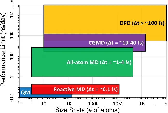
Figure 1.1. Performance limit (simulation time per day) vs system size scale for various molecular modeling methods. The highest resolution methods in the lower left corner describe systems with the most detail, but these systems also have the lowest performance limit and system size. As size scale increases, the systems are described for less detail, and the performance limit increases due to the increased timesteps (Δt) that are possible when describing a system with less detail. The bottom of the image shows snapshots depicting the application of various computational methods to the NP−nucleic acid interface... 20

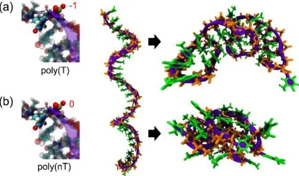
Figure 2.1. Representative initial and last simulation snapshots in this study. Total charge on the phosphate group (left), snapshot of the initial (center) and a final (right) structures of (a) regular poly(T)20, (b) neutral polyT, poly(nT)20 ... 39

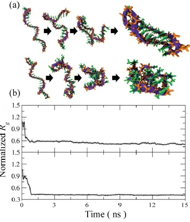
Figure 2.2. (a) Representative folding pathway of 25-mer ssDNA in implicit solvent for the first 15 ns. Simulation snapshots illustrating a typical folding where backbone represented as a purple ribbon and backbone atoms are orange and base atoms are green. (b) Temporal profile of normalized radius of gyration for poly(T)25 (top) and

poly(nT)25 (bottom) ... 40

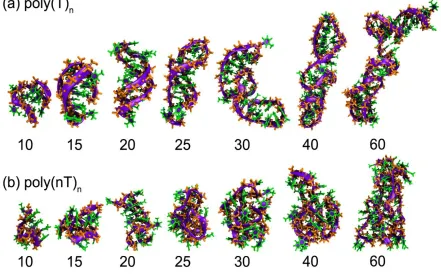
Figure 2.3. Simulation snapshots of (a) poly(T)n and (b) poly(nT)n representing equilibrated

(16)

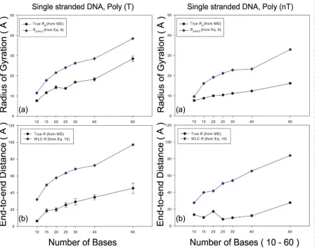
Figure 2.4. Radius of gyration (Rg) and end-to-end distance (R) of poly(T) and poly(nT). True Rg, and R calculated from MD simulations are colored by black circles. Estimated Rg,WLC and RWLC for poly(T) and poly(nT) are navy diamonds. ... 42

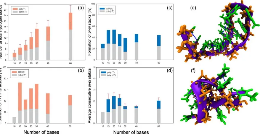
Figure 2.5. Formation of specific non-bonded interactions in poly(T) (orange or blue bars) and poly(nT) (grey bars). (a) Total number of hydrogen bonds; (b) percentage of non-Watson-Crick T-T base-pairing; (c) percentage of pi-pi stacks; and (d) number of consecutive pi-pi stacks. Snapshots of (e) poly(T)15 and (f) poly(nT)15. Blue thick

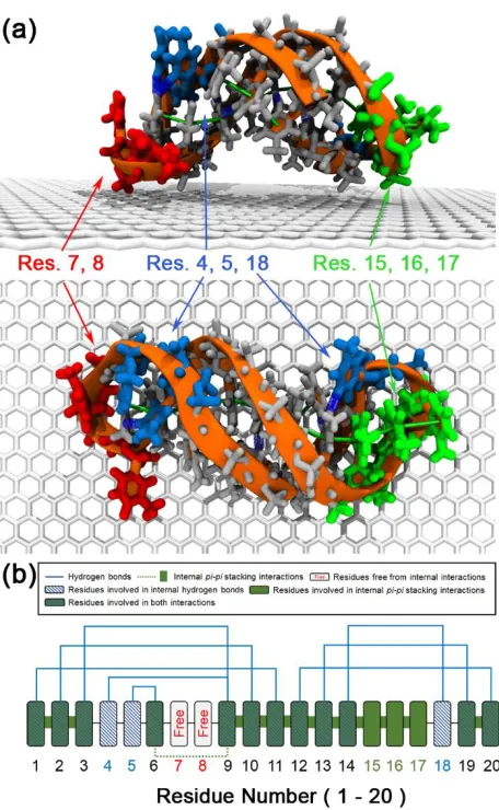
lines represent formation of pi-pi stacks, and red dotted lines indicate the T–T base pairings. ... 43 Figure 3.1. (a) Representative side and top view snapshots of initial conditions of pre-folded

poly(T)20 on the graphene-based surface. DNA is represented by orange tube with

white colored nucleobases. Green, blue, and red colored residues highlight the regions where nucleobases are involved in only pi-pi stacking interaction (green), internal hydrogen bonds (blue), both of them (Gray), or not involved in the internal interactions (red), respectively. (b) Detailed information on internal non-bonded interactions of poly(T)20. ... 67

(17)

Figure 3.3. (a) Representative snapshot of the initial structure of poly(T)20 on graphene-based

surfaces with an axis normal to the surface (z-axis). (b) Atomic density profile (solid red line) of poly(T)20 atoms along z-axis over last 10 ns of 100 ns-simulation

trajectories with red shaded regions representing standard deviation. Gray dotted lines represent density profile of the initial structure prior to adsorption depicted in (a). ... 69 Figure 3.4. (a) Number of poly(T)20 atoms participating in hydrophobic contacts with the

surface. (b) An average number of pi-pi stacking interactions between DNA bases (base stacking, black circles) and between DNA bases and graphene-based surfaces (base-surface stacking, blue squares). Red dashed line indicates the number of base stacks in initial poly(T)20 structure. ... 70

Figure 3.5. (a) Schematic of various non-bonded interactions observed during physisorption of poly(T)20 on graphene-based sur-faces. (b-f) Probability heat map (%) of

(18)

view and side view of poly(T)20 snapshots on GO 5%, GO 15%, and GO 40% as a

representation for the case with low, moderate, and high oxygen content, respectively. Green colored surfaces in the snapshot illustrate regions where close DNA – carbon surface contacts are found. ... 71 Figure 3.6. (a) Representative snapshot of poly(T)20 and (b) its density profile on the regular

GO20% (left) and on nGO20% (right). Average values (red lines) and standard deviations (red shaded regions) were taken from last 10 ns of 100 ns-simulations. Comparison of probability heat map for (c) internal hydrogen bonds, (d) base-base stacking interactions, and (e) interfacial hydrogen bonds (red), and pi-pi stacking interactions (cyan) among initial poly(T)20 structure (Int), GO 20%, and nGO 20%

case. ... 72 Figure 4.1. Root mean square deviations of poly(T) (black), poly(A) (red), and poly(AT)

(blue) on (a) pristine graphene, (b) GO 5 %, (c) GO 10 %, (d) GO 15 % and (e) GO 20% as a function of time. ... 90 Figure 4.2. Simulation snapshots of (a) poly(T)20, (b) poly(A)20, and (c) poly(AT)10 adsorbed

(19)

Figure 4.3. Persistence length of poly(T)20 (black squares), poly(A)20 (red circles) and

poly(AT)10 (blue triangles) as a function of oxygen coverage of the surface. Black,

red, and blue dashed lines represent a regression line of poly(T)20, poly(A)20, and

poly(AT)10, respectively. Gray dotted line means persistence length of poly(T)20 in

0.5 M NaCl solution. ... 92 Figure 4.4. Internal non-bonded interactions of ssDNA: (a) the number of hydrogen bonds

between nucleobases, (b) the number of base-base stacking interactions. Numbers inside plots represent oxygen coverages of the surface (%) ... 93 Figure 5.1. Schematic of the CR-AFM setup. The AFM tip can be approximated as a sphere

with radius R indenting the sample. ... 122 Figure 5.2. (a) Optical microscopy and (b) AFM topographic images of a typical few layer

graphene on UDT. The red arrows indicate the region where point measurements were made. (c) Raman spectra of graphene on CH3-(black, UDT) and NH2-SAMs

(blue, AUT). (d) 2D FWHM comparison of graphene on CH3- and NH2-SAMs for

both as-prepared samples and samples after vacuum annealing. ... 123 Figure 5.3. Contact resonance frequencies of FLG-CH3-SAM (black) and FLG-NH2-SAM

(blue) heterostructures: (a) for as-prepared samples and (b) for samples after vacuum annealing. (c) and (d) are the corresponding Raman 2D peak position for both samples before and after vacuum annealing, respectively. ... 124 Figure 5.4. (a) Representative MD snapshots of FLG on SAM with –NH2 (top) and –CH3

(20)

between FLG and SAM with –NH2 (blue) and –CH3 (black) head groups. Average

values over the last 10 ns of the simulations are inserted as bar graphs. ... 125 Figure 5.5. (a) Simulated stress – strain curves for FLG-NH2-SAM and FLG-CH3-SAM

heterostructures in ambient (top) and vacuum conditions (bottom). (b) Estimated Young’s modulus for each case. (c) Representative snapshots of steered MD

simulations. The images from top to bottom correspond to regimes I, II and III of a FLG-CH3-SAMs heterostructure in vacuum. ... 126

Figure 5.6. (a) Schematic showing the components of non-bonded interactions that are present in the SAM-FLG system: Interfacial non-bonded interactions between FLG and SAMs (green), inter-chain interactions among SAMs (blue), inter-chain interactions with only the alkyl chains (i.e., without head groups, orange), graphene (bottom layer only) – water interactions (gray), and interactions between water and the SAM (red). Deconvolution of the non-bonded interaction energy determined for (b) the FLG - CH3 SAMs and for (c) the FLG - NH2 SAMs in compression

regime I. ... 127 Figure 5.7. Histogram of the nearest neighbor distances (head group to head group) in

compression Regime I, for a CH3-SAM in (a) ambient conditions, and (b) in

vacuum, and for a NH2-SAM in (c) ambient conditions, and (d) in vacuum. The

(21)

Figure 6.1. AFM topographical images of silk fibroin absorbed from 0.2 (A), 0.02 (B), and 0.002 wt. % (C) SF deposited on GO flakes via conventional SA-LbL at 5000 rpm. Scale: 500 nm. Z range: 4 nm (A and C) and 5 nm (B). ... 174 Figure 6.2. AFM topographical images of 0.002 wt. % silk fibroin morphology after

conventional SA-LbL on SiO2 surface (A, C, E) and GO flakes (B, D, F) on Si wafer

at 3000 (A, B), 5000 (C, D), and 8000 (E, F). Scale: 2 um. Z range: 2 nm (A, C, and E), 3 nm (B), 6 nm (D), and 3 nm (F). ... 175 Figure 6.3. AFM topographical images of 0.002 wt.% silk fibroin morphology after dynamic

casting on GO flakes on silicon wafer at 1000 (A), 2000 (B), 3000 (C), 4000 (D), 5000 (E), and 8000 (F) rpm. Scale: 500 nm. Z range: 2 nm (A, B, D, E, and F) and 9 nm (C). ... 176 Figure 6.4. AFM topographical images of 0.002 wt.% silk fibroin morphology after

conventional SA-LbL on rGO flakes on a silicon wafer at spin speeds 3000 (A), 5000 (B), and 8000 (C) rpm. Scale: 500 nm. Z range: 7 nm (A), 11 nm (B), and 28 nm (C). ... 177 Figure 6.5. AFM topographical images of 0.002 wt.% silk fibroin morphology after dynamic

spin casting on rGO flakes on a silicon wafer at spin speeds of 1000 (A), 2000 (B), 3000 (C), 4000 (D), 5000 (E), and 8000 (F) rpm. Scale: 500 nm. Z range: 8 nm (A and C), 11 nm (B and E), 2 nm (D), and 12 nm (F). ... 178 Figure 6.6. ATR-FTIR spectra of SF (A), SF-GO (B), and SF-rGO (C) in the amide 1 region.

(22)

Figure 6.7. (a) Density profile of silk atoms normal to the graphene (black), GO 20% (blue), SiO2 (red), and the initial silk structure on GO 20% (gray dotted line). (b) Final

snapshot of each case in (a). (c) Density profile of silk parallel to the surfaces where the initial structure is indicated by black lines. ... 180 Figure 6.8. (A) β-sheet content per each silk residue. (B) Temporal profile of the percentage

of random coils (black) and ordered structures (gray) in silk structure. Yellow and red lines passing through the black and gray lines indicate the averaged values of the percentage of random coils and ordered structure, respectively. ... 181 Figure 6.9. MD simulation (A) and experimentally (C) observed changes in secondary

structure of silk on three different surfaces: graphene (rGO for experimental results), GO with 20 wt. % oxygen coverage, and SiO2. ... 182

Figure 6.10. (A) Temporal profiles of van der Waals contributions (green), electrostatic interactions (red) and total non-bonded energy (black) between silk and graphene (left), GO (center), and SiO2 (right). (B) Temporal profiles of the number of internal

hydrogen bonds for silk protein on graphene (left), GO (center), and SiO2 (right)

surface, where averaged values for silk protein and silk protein-surface hydrogen bonding are represented by black and gray lines, respectively. ... 183 Figure 7.1. Structure of Candida antarctica lipase B drawn as (a) a cartoon model and (b) Van

der Waal’s surface. The α-10 helix region (residues 268 to 287) is represented as

(23)

Figure 7.2. Depth profiles of the catalytic cavity calculated from the interior of the enzyme towards the surface for (a) [Bmim][TfO], (b) tert-butanol, (c) [Bmim][Cl], (d) 0.3M NaCl solution, with representative snapshots of CALB from MD simulations (ILE-189 and ILE-285 are dark gray). Black thick line is the cavity profile of CALB crystal structure. Average value from simulations is shown as thin gray line. The approximate positions of cavity entrance at ~16 Å and catalytic triad position at ~6 Å are shown by dotted lines. ... 213 Figure 7.3. The conversion rate of lipase-catalyzed trans-esterification of butyl alcohol with

vinyl acetate in (a) [Bmim][TfO], (b) tert-butanol, (c) [Bmim][Cl]. ... 214 Figure 7.4. (a) Snapshot of CD1 atom positions in ILE-189 and ILE-285, which limits the

width of catalytic cavity (b) Calculated probability distribution of the width of catalytic cavity entrance in different solvent systems. Dashed line indicates the distance between ILE-189 and ILE-285 in the crystal structure (7.294 Å ). ... 215 Figure 7.5. Average root mean squared deviation for each residue in four types of solvents

evaluated from 100 ns simulation. Shaded gray region represents α-10 helix region

(residue: 268-287), and also show high RMSD peak in all solvents except for [Bmim][TfO]... 216 Figure 7.6. The interaction between chlorine anions and LYS-290 of CALB in [Bmim][Cl].

The snapshots were taken when cavity was (a) in the open conformation and (b) in the closed conformation where bonding is shown as a dotted line. ... 217 Figure 7.7. The correlation between experimentally observed initial reaction rate of butyl

(24)

between solvents and surface of CALB in various solvents. Dashed line indicates regression fit... 218 Figure 8.1. Illustration of chemical structure of (a) cations: [Emim]+, [Bmim]+, [Hmim]+,

[Omim]+ and (b) anion: [TfO]- used in this study. (c) Crystal structure of CALB represented as a surface model where ILE-189 and ILE-285 are colored red, LYS-290 (KLYS-290) is green and catalytic triad (SER-105, ASP-187, HIS-224) is blue. (d) Calculated coordination number of cations and (e) snapshots of representative coordination from simulations of ILs. ... 246 Figure 8.4. Snapshots of the part of α-10 helix region in (a) [Emim][TfO], (b) [Bmim][TfO],

(c) [Hmim][TfO], and (d) [Omim][TfO]. Red and blue colored molecules represent anion and cation within 3.0 Å of LYS-290, respectively. LYS-290 is illustrated as Van der Waals spheres and two gate residue, ILE-189 and ILE-285 are drawn as licorice models covered with transparent red surface models representing gate conformations. (e-h) The temporal number of cation and anion within 3.0 Å of LYS-290 in (e) [Emim][TfO], (f) [Bmim][TfO], (g) [Hmim][TfO], and (h) [Omim][TfO]. Red and blue lines represent anion and cation, respectively. ... 249 Figure 8.5. (a) Side-view of α-10 helix in [Emim][TfO] (left) and in [Omim][TfO]. Cation is

illustrated by blue colored licorice model. α -10 region and HIS-224 is colored by

(25)

Figure 8.6. (a) A snapshot of α-10 helix region and the position of LEU-278 and ALA-282 of CALB in [Emim][TfO] (upper), and [Omim][TfO] (lower). LEU-278 and ALA-282 are represented as licorice model colored by atom name. Green dotted line illustrates a hydrogen bond. (b) Temporal profile of the number of hydrogen bonds between LEU-278 and ALA-282. (c) A snapshot of catalytic cavity of CALB in [Omim][TfO] and [Omim]+ (blue), [TfO]- (red) molecules within 3.0 Å of catalytic triad (yellow). (d) Temporal profile of the number of [TfO]- within 3.0 Å of HIS-224 in ILs. ... 251 Figure 8.7. Correlation between geometrical stability of catalytic triad (black circles), most

probable distance between two gate amino acids (D189-285, blue squares) and initial reaction rate. Red shaded region represents closed gate conformation of CALB in [Emim][TfO]. Regression lines of the cases with open conformations are shown as grey and blue dashed lines. ... 252 Figure 9.1. (a) Front view (top) and Top view (bottom) of the crystal structure of CALB with

an opaque and transparent 3-D surface model, respectively. Amino acids mentioned in this study including catalytic triad (S105, D187, H224), mutation sites (D223, S227), red gate (I189 and I285), and green gate (E188, L278) are highlighted as colored surface models. (b) An overview of combined experimental and computational approach used in this study. ... 279 Figure 9.2. Probability heat map of distance between gate residues regulated by ILE189 –

(26)

indicating a size of the red gate and green entrance are illustrated top and right-side of the heat map, respectively. Representative snapshots for each case are also shown in this figure. For the snapshots, same color codes shown in Figure 1a are used to highlight important residues in CALB. ... 280 Figure 9.3. (a) Representative snapshots illustrating H224 – 188 hydrogen bonding interaction

(top) and hydrogen bonding occupancy (%) of H224 – 188 interaction observed in WT and its variants (bottom). (b) Representative snapshots of a-10 helix region in WT and D188E mutant (top). Hydrogen bonding occupancy (%) of L278 – A282 (green), L278 – A281 (brown), and L278 –A274 (orange) (bottom). (c) A correlation between the solvent accessible surface area of catalytic triad and relative BZA activity of WT and its variants with snapshots of CALB representing buried, partially exposed and fully exposed catalytic triad. ... 281 Figure S 2.1. Partial charge of thymine monomer of (a) regular ssDNA, poly(T), (b) neutral

ssDNA, poly(nT), Neutralized oxygen atoms for poly(nT), OP1 and OP2 are colored as red and reference atoms for the vector calculation, O3’ are illustrated as

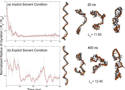
blue………44 Figure S 2.2. Comparison between folding pathway and persistence length (Å ) of poly(T)40

via (a) implicit solvent simulations (60 ns) and (b) explicit solvent simulations (400 ns). Each snapshot represents folding dynamics of poly (T)40 at both 0.5 M implicit

(27)

Figure S3.1. (a) Snapshots of graphene-based surfaces used in this study. Blue and red colors on the surfaces represent partial charges of functional groups. The charged functional groups bond with both the top and bottom surfaces of the sheet... 73 Figure S3.2. Simulation setup. (a) The initial position of poly(T)20 structure on graphene-based

surface in the water box. (b) Top view of initial position of poly(T)20 on

graphene-based surface. (c) Partial charges used for hydroxyl and epoxy groups. (d) RMSD of free poly(T)20 solvated in 0.5 M NaCl solution. ... 74

Figure S3.3. (a) Top view and (b) side view of representative snapshots of poly(T)20

conformation on various graphene-based surfaces. Green color surfaces represent close contact regions between carbon atoms on a graphene sheet and DNA atoms. ... 75 Figure S3.4. Temporal profiles of non-bonded energy between poly(T)20 and various

graphene-based surfaces. ... 76 Figure S3.5. Temporal profiles of VDW energy between poly(T)20 and various

graphene-based surfaces. ... 77 Figure S 3.6. Temporal profiles of electrostatic (ELEC) energy between poly(T)20 and various

graphene-based surfaces. ... 78 Figure S3.7. Temporal profiles of the hydrogen bonds between poly(T)20 and various

graphene-based surfaces. ... 79 Figure S 3.8. Estimated binding free energy differences between poly(T)20 and the surfaces.

A yellow circle at GO 20% case illustrates binding free energy of poly(T)20 on

(28)

Figure S3.9. Comparisons of multiple simulations: simulation 1 is the case with poly(T)20 on

the graphene-based surface, which are introduced in the manuscript; simulation 2 is additional MD simulation with poly(T)20 on the surface with different distribution

of oxidation groups (a) Side and top view of representative simulation snapshots, (b) atomic density profile of poly(T)20 atoms along the axis perpendicular to the

surfaces, (c) stacking and hydrogen bonding interactions observed in the cased of PG, GO20%, and 60% (Gray bars) and their flip sides of the surfaces (Red bars). ... 81 Figure S 5.1. Beam model of the AFM cantilever in contact with a sample surface... 129 Figure S 5.2. Partial charge information on (a) 1-undecanethiol (-CH3), (b)

11-amino-1-undecanethiol (-NH2), and (c) protonated 11-amino-1undecanethiol (-NH3+) used

in this study. ... 130 Figure S 5.3. Elastic modulus as a function of indentation speed (v), 0.05, 0.001, and 0.00001

pN/time step. (a) Stress – strain curve in compression regime I. The negative strain in the beginning part of some of the curves is due to FLG-SAM force fluctuations when the applied stress is low. (b) Elastic modulus values with corresponding R2 values (number inside the bar graphs) obtained from the slopes in the linear compression regime for three different indentation speeds, and (c) comparison between reduced modulus values from the experiment and averaged modulus values from SMD simulations. ... 131 Figure S 5.4. Temporal profiles of the overall interfacial interaction energy between (a) FLG

(29)

regime I. Dark colored and light colored bars with step value (t) illustrate the approximate yield point. Temporal profiles of inter-chain interactions among (c) CH3 and (d) NH2 terminated SAMs. The dotted lines represent the profiles of

inter-chain interactions of alkyl inter-chains without head groups. ... 132 Figure S 5.5. High resolution N 1s XPS shows the protonation of amine groups in the NH2

-SAM ... 133 Figure S 5.6. Raman spectra of bulk HOPG. The blue arrow indicates the characteristic

shoulder of the bulk HOPG 2D peak, which does not show up in the FLG samples. ... 134 Figure S 5.7. Time evolution of the non-bonded interaction energy between SAMs and

interfacial water (red), SAMs and surrounding water (water molecules within 4.5 Ȧ of head groups excluding interfacial water, blue), the bottom layer of FLG and

water (gray), and the entire SAM and water molecules (black). ... 135 Figure S 5.8. (a) Representative simulation snapshot of FLG on NH3+-SAMs in water. In this

snapshot, water molecules are omitted. (b) Average number of water molecules and (c) average non-bonded interaction energy between FLG and –NH3+ head groups.

... 136 Figure S 5.9. Non-bonded interaction energy between FLG and –CH3 head groups, –NH2 head

groups, and –NH3+ head groups in vacuum condition. ... 137

Figure S 5.10. Schematic showing the presence of water in the vicinity of the FLG-CH3-SAM

(30)

-terminated SAM when graphene is transferred to the SAM surface in ambient conditions. (b) Top view, showing that the SAM is a polycrystalline structure, with some grain boundaries and defects, where water (blue) can be present (The image is modified from a STM image of a CH3-terminated alkanethiol SAM on Au (111)).

The MD simulations simplify this complex scenario into a patch of the FLG-SAM heterostructure with surrounding water molecules and periodic boundary conditions. ... 138 Figure S 6.1. Silk fibroin at 0.002 wt. % dynamically cast on GO flakes at 5000 rpm

morphology in AFM height (A) and phase (B) images with height profiles corresponding to the white (C), red, green, and blue lines (D) in A. Scale: 100 nm. Z range: 2 nm. ... 184 Figure S 6.2. Silk fibroin at 0.002 wt. % deposited via conventional SA-LbL on GO flakes at

5000 rpm morphology in AFM height (A) with height profiles corresponding to the red, green, and blue lines (B) in A. Scale: 100 nm. Z range: 10 nm. ... 185 Figure S 6.3. ATR-FTIR spectra of silk fibroin (A) on GO (B) and rGO (C) in the amide I and

amide II regions. ... 186

Figure S 6.4. Sequence of Bombyx Mori heavy chain with 258-amino acid segment used in MD simulation. ... 187 Figure S 6.5. XPS of rGO carbon peak for hydrazine solution (A) and vapor reduction methods

(B). ... 188 Figure S 6.6. Ramachandran plot with the probability (I) of silk on (A) graphene, (B) GO, (C)

(31)

Figure S 7.1. Chemical structure of solvents used in this study. (a) 1-Butyl-3-methylimidazolium ([Bmim]+), (b) Trifluoromethanesulfonate ([TfO]-) and (c) tert-butanol. ... 222 Figure S 7.2. The production yield of butyl acetate after 12 h reaction in [Bmim][TfO], tert-butanol and [Bmim][Cl]. ... 223 Figure S 7.3. Root mean square deviation (RMSD) of CALB that was calculated for backbone

atoms as a function of time during 100 ns in [Bmim][TfO] (Red), tert-butanol (Blue), [Bmim][Cl] (Green), and 0.3M NaCl solution (Black). ... 224 Figure S 7.4. (a) Snapshot of CD1 atoms of ILE-189 and ILE-285, and (b-e) temporal profiles

of the distance between CD1 atoms in ILE-189 and ILE-285 in (b) [Bmim][TfO], (c) tert-butanol, (d) [Bmim][Cl], and (e) 0.3M NaCl. Average profile is shown as black line. A black dotted line indicates the threshold distance. ... 225 Figure S 7.5. Conformational changes of the alpha-10 helix region in various solvents (a)

initial X-ray crystal structure, (b) [Bmim][TfO], (c) tert-butanol, (d) [Bmim][Cl], (e) 0.3M NaCl (Open), (f) 0.3M NaCl (Closed). Region with significant conformational changes is shown in red. ILE-189 and ILE-285 are shown as stick molecular model... 226 Figure S 8.1. Root mean square deviation (RMSD) of CALB solvated in [Emim][TfO] (black),

[Bmim][TfO] (Red), [Hmim][TfO] (Dark green) and [Omim][TfO] (Blue) ... 256 Figure S 8.2. Radial distribution function of carbon atom in imidazolium cation. [Emim]+

(black), [Bmim]+ _{(red), [Hmim]}+ _{(green), and [Omim]}+ _{(blue). Second solvation}

(32)

Figure S 9.1. (a) Model enzyme reactions used in this study. (b) Simulation box composed of the organic molecule mixtures: 3:1:1:1 ratio of 1-octanol (orange), 1-otanoic acid (blue), 2-ethylhexanoic acid (yellow), and benzoic acid (green). CALB is located in the middle of the box. ... 283 Figure S 9.2. Comparison between conventional computational approaches (case 1 and 2) and

(33)

Introduction

*A portion of this chapter is based on two manuscripts by (1) Jessica A. Nash, Albert L. Kwansa, James S. Peerless, Ho Shin Kim, and Yaroslava G. Yingling and (2) Nan K. Li, Ho Shin Kim, Jessica A. Nash, Mina Lim, and Yaroslava G. Yingling, which were published by following two journals as review papers, respectively: Bioconjugated Chemistry (2017) and Molecular Simulations (2014).

1.1 Background and Motivation

1.1.1 Understanding Single Stranded DNA: From Structure and Dynamics to

Physisorption on the surfaces

(34)

ssDNA conformation. For these reasons, more detailed and atomistic approaches are needed to precisely estimate structure and dynamics of ssDNA.

It is also imperative to understand structure and dynamics of ssDNA functionalized with surfaces in various conditions such as surface polarity because, for aforementioned applications using ssDNA, it is integrated with the surfaces.[8]_{Generally, the surface polarity}

is known to be an important factor for the adsorption process,[9-10]_{structure, and dynamics of}

biomolecules.[11]_{Recently, graphene surfaces are known for their excellent mechanical}

strength,[12-13]_{large surface area,}[14]_{and unique bonding networks}[15-16]_{. Moreover, oxidation}

of graphene surfaces permits controlled modification of surface polarity and hydrophobicity. Due to their unique properties, pristine graphene (PG) and its oxidized surface, graphene oxide (GO), have been used in many applications, including water purification process,[17]

antimicrobial treatments,[18]_{and bionanocomposites.}[19-20]_{It is known that DNA adsorption on}

graphene surfaces is a complex process and depends on local sequence variations, defects, and surface properties.[21]_{However, fundamental understanding of how surface polarity affects}

ssDNA structure is unclear and remains to be explored, even though GO is considered to have better biocompatibility than PG due to its amphiphilic behavior.[22-23]_{For other biomolecules,}

such as proteins, it has been reported that there is an incomplete agreement of the relation between surface polarity and compatibility or stability of biomolecules on these surfaces.[24-26]

For DNA-surface interactions, the significance of two important bonding contributors for the physisorption of ssDNA on graphene-based surfaces, e.g. pi-pi stacking interactions and hydrogen bonds, has been emphasized in previous studies.[8, 27-28]_{Aforementioned studies}

(35)

have a direct implication on physisorption process and these interactions can either enhance or reduce biocompatibility and stability of ssDNA on graphene-based surfaces. However, a systematic investigation of the surface polarity that influences these important interactions has not been performed and the underlying processes of DNA binding to surfaces still unclear as the published studies are controversial. For these reasons, more detailed and atomistic approaches are needed to precisely estimate structure and dynamics of ssDNA on graphene based surfaces.

A part of this dissertation (Chapter 2, 3, and 4) describes simulation results designed to address and elucidate (1) how charge, base, and length of ssDNA affect its structure and dynamics and (2) how surface polarity of graphene-based surface influence structure and dynamics of ssDNA while it is adsorbed on the surfaces.

1.1.2 Combined computational and experimental study for understanding

Graphene-based Surfaces for their applications: Mechanical properties and physisorption with

proteins for bionanocomposites

(36)

variety of inorganic or carbon components. Carbonaceous additives such as graphene and carbon nanotubes provide greater mechanical strength to the composite and electrical properties necessary for sensing and energy storage devices while the elastomeric biomaterial matrix can confer flexibility and biocompatibility. However, extraordinary mechanical properties of silks nanocomposites depend on many factors such as silk sequence, secondary structure formation, local microstructure, and surface polarity. For these reasons, understanding of interfacial interactions between silk fibroin structure and graphene-based surface needs to be clear to obtain optimal mechanical properties of silk nanocomposites under the various conditions.

As mentioned earlier, graphene has been spotlighted as a promising material for a variety of devices, including biosensors, touch screens, and flexible electronics.[42-44] For these applications, graphene is usually supported by a substrate because it enables the device to function effectively and enhances the mechanical stability of graphene. Self-assembled monolayers (SAMs) are used as an effective interfacial layer to modify a substrate surface to mitigate unwanted substrate effects. However, different SAMs will have different interactions with graphene. For example, the adhesion energy depends on (1) the SAM head group identity,[45]_{(2) the interfacial layer formed between graphene and the SAM during the}

preparation process, and (3) the graphene-SAM separation distance.[46] However, how SAMs, and especially their surface energy, affect the mechanical properties at the interface between graphene and a substrate is not yet known. Moreover, the out-of-plane elastic modulus of a layered graphene heterostructure is interrelated with graphene’s thermal, electrical,

(37)

interfacial interactions. However, to date little is known about the out-of-plane elastic modulus of graphene and other 2D materials, as the measurement of modulus changes due to differences in 1, 2 atomic or molecular layers. Hence, precise characterization of the out-of-plane elastic modulus is important for both fundamental research and practical applications.

A part of this dissertation (Chapter 5 and 6) describes combined experiment (achieved by research collaborators) and simulation results designed to address and elucidate (1) an effect of surface polarity on secondary structures of silk-fibroin structure and (2) an role of interfacial condition between graphene and self-assembled monolayer on its mechanical properties.

1.1.3 Increasing lipase activity through computational modeling: Structure-activity

relation of Candida antarctica Lipase B and its mutants in various solvents.

(38)

commercial products in various markets from benzoate ester plasticizers for PVC products to benzoate ester emollients and solubilizers in personal care products. Since these branched or sterically demanding substrates are required as sources for the high-value products, it is imperative for us to overcome these drawbacks and find a means to specifically increase the ability of enzymes to react with bulky acids. Also, even though CALB is a very stable enzyme in various solvents, the choice of solvent can be crucial for enzyme activity. For example, CALB can lose its activity and structural stability in ionic liquids (ILs) containing strongly coordinating anions, such as acetates or halides (e.g., Cl-_{, Br}-_{, or I}-_{), whereas ILs with weakly}

coordinating anions, such as [TfO]-_{or [Tf2N]}-_{can enhance CALB’s activity. Overall,}

aforementioned two factors, the effect of (1) solvent and (2) specific amino acid changes in enzyme activity need to be elucidated in order to improve enzyme activity and stability.

A part of this thesis (Chapter 7, 8, and 9) describes combined computational and experimental results designed to address and elucidate the effect of the choice of (1) ionic solvents (2) amino acids for point mutations on enzyme activity of CALB resulting from their structural changes.

1.2 Methods

(39)

well-tested methods and force fields exist to study various biomolecules including protein, enzymes, and nucleic acids, and recent advances in computing algorithms and architecture, such as the use of graphics processing units (GPUs), allow for the simulation of increasingly large and complex systems. For instance, a single GPU-accelerated server can provide a comparable computational throughput to ~50 CPU-only servers at a markedly reduced cost and power utilization.[48]_{Consequently, simulation methods show tremendous potential for providing}

important details of bio-molecules under various conditions.

(40)

1.2.1 All-atom Molecular Dynamics Simulations

All-atom MD simulations can provide a complete microscopic description of the structure and dynamics of biomolecules under different environmental conditions, from detailed information on atom-to-atom interactions via hydrogen bonding or pi-pi stacking to atom interactions with ions, small molecules, and proteins to global functionally important motions and conformational changes which control the processes of self-assembly. As aforementioned, using an accurate force field and efficient algorithm detailed all-atom investigation can shed the light on structure and dynamics of biomolecules under the various conditions.[58-59]

All-atom MD simulations neglect the electronic nature of molecules and instead model atoms as spheres connected by spring-like bonds, which move according to Newton’s equations of motion (Please note that all subsequent use of “traditional MD” or “all-atom MD” refers specifically to all-atom non-reactive MD).[60]_{For a system composed of}_N_particles,

classical Newton’s equations of motion are:

,

In this equation, Fi represents the force acting on the ith particle, mi is the mass of the particle, and ai is the acceleration, U is potential energy and ri is a position of ith particle. The potential energy U can be classified into two groups:

Where Unon-bondedis the contributions total energy from non-bonded interactions among particles including electrostatic or van der Waals interactions and Ubondedrepresents the total

i i i

i U F m a

r 

  

 i1, 2,3, 4... N

(41)

bonding potentials such as changes in bonds, angles, and dihedrals. The results of the atomistic simulations are strongly dependent on the accuracy of the force field which is a combination of a mathematical formula and parameters to describe the energy as a function of their atomic coordinates.[61] For example, general form of the total energy in the AMBER[62-63] force fields which are the most frequently used in this work are written as:

(Bonded)

(Non-bonded)

Where kb is a bond spring constant, rij=|rj – ri| gives the distance between two atoms i and j, req is the equilibrium bond distance, ka is an angle constant, θijk is angle between rij and rjk, θeq is the equilibrium angle, kn_{is the multiplicative constant, n is the integer constant, ω is} the phase shift angle, γ is an equilibrium torsion angle, Ɛij is the potential wall-depth, Q is the

charges on the respective atom, i and j. Several different all-atom force fields have been developed for biomolecules, including CHARMM[64], AMBER[62-63], Bristol-Myers Squibb (BMS)[65], and GROMOS.[66]

There are several numerical methods to solve or integrate Newton’s equation of motion,

such as Verlet,[67] Leap-Frog, and Velocity Verlet alogorithm. For the Verlet algorithm, which is a foundation of other numerical methods, the solution of Newton’s equations of motion is based on a Taylor series expansion. Expanding the position of ith particle ri at time t+∆t and t

2 2 1

( ) ( ) ( ) [1 cos( )]

2

N n

b ij eq a ijk eq

BONDS ANGLES DIHEDRAL n

U r 



k r r 



k   

 

k  n 

12 6

0 0

1 1 0

2

4 ij ij i j ij ij

i j i ij ij ij

r r Q Q

f

r r r

(42)

– ∆t, adding two equations, solving ri(t+∆t), and using Newton’s equations for the acceleration, leads to:

However, the Verlet algorithm has issues related to the velocity: (1) the velocity does not explicitly appear in this algorithm and (2) it is hard to calculate the velocity at time tn until the position at time ri(t+∆t) is obtained.[68]_{In order to correct aforementioned issues related}

to the velocity, other numerical methods including Leap-Frog and Velocity Verlet algorithms have been developed and widely used in MD simulations.

When performing all-atom MD simulations of biomolecules, choosing an appropriate solvent model is also an important factor. Explicit solvent models, where solvent particles are included in the simulation, have been most widely used, and non-polarizable fixed-charge models have been the most prevalent.[69] Explicit solvent can afford the prediction of important solvent effects such as solute-solvent interactions. However, due to the increased number of simulated particles, considerable computational resources are required to simulate systems containing explicit solvent.[70] Moreover, careful parameterization is required to represent solvents and solute-solvent interactions accurately and the choice of the force field for solvent becomes imperative.[71] Even for water alone, there are many different all-atom models that have been developed, including the most frequently used OPC[72], SPC[73], SPC/E[74], TIP3P[75], TIP4P[76], and TIP5P[77], all of which are able to represent different properties of water with different degrees of accuracy. In explicit solvent simulations, the choice of force field parameters for salts is also important, since nucleic acids are charged molecules. For example,

2

4

( ) 2 ( ) ( ) ( ) ( )

i i i

t

r t t r t r t t F t O t

m 

(43)

incorrect parameterization of monovalent ions has led to incorrect results, or conclusions in simulation studies based on artifacts.[78]

Implicit solvent models for all-atom simulations, where the solvent is treated as a continuum dielectric with the average properties of real solvent, can significantly reduce computational expense due to the reduced number of simulated particles and their associated degrees of freedom; furthermore, the absence of viscosity increases rate at which the solute explores its conformational space and reduces the real-world time needed to capture such dynamic processes.[79-81]_{However, implicit solvent models cannot capture, e.g., viscosity}

effects[82] and specific solute-solvent interaction mechanisms.[83] In this dissertation, TIP3P water model for most studies and generalized born implicit solvent model for some initial studies were used.

1.2.2 Steered Molecular Dynamics Simulations

Steered MD simulations (SMD) carry out MD simulations and additionally exert a pulling forces to atoms or molecules. This simulation technique can not only accelerate simulation process accompanying structural changes by forces acting on the structure, but also estimate many informative structural and mechanical properties of structures, such as Young’s modulus and persistence length.

(44)

Where ks is a spring constant, v is a pulling velocity, t is a time, n is a direction of pulling and a vector r and r0 is an actual and initial position of the atom or molecule of interest, respectively.

This method is mainly used in Chapter 5 in order to estimate the mechanical properties (i.e. Young’s modulus) of a graphene surface on self-assembled monolayer with two different

interfacial conditions.

1.3 Publications

Publications listed below is the review, research papers, and patent that I have published during my Ph.D. study or I plan to publish soon. Each chapter is based on or refers to the following publications:

Chapter 1

- N. K. Li, H. S. Kim, J. A. Nash, M. Lim, & Y. G. Yingling. "Progress in molecular modelling of DNA materials." Molecular Simulation, 40, (2014): 1-7

- J. A. Nash, A. L. Kwansa, J. S. Peerless, H. S. Kim, & Y. G. Yingling. “Advances in molecular modeling of nanoparticle-nucleic acid interfaces, Bioconjugate Chemistry, 28, 1 (2017): 3-10

- B. Roark, A. Ivanina, J. Castaneda, H. S. Kim, S. Jawahar, M. Viard, S. Talic, Y. G. Yingling, M. Jones, & K. Afonin. "Fluorescence blinking as an output signal for programmable biosensing", ACS Sensors, 1, 11 (2016): 1295-1300

U F r     2 0 1 ( ) ( ) 2 s

(45)

Chapter 2

- H. S. Kim, A. Singh, & Y. G. Yingling. "Understanding the persistence length of single stranded DNA: atomistic molecular dynamics simulations” In preparation for submission (2017)

Chapter 3

- H. S. Kim, B. L. Farmer, & Y. G. Yingling. “Effect of graphene oxidation rate on adsorption of poly-thymine single stranded DNA”, Advanced Materials Interfaces, 4, 8 (2017): 1601168

Chapter 4

- H. S. Kim, S. M. Huang, & Y. G. Yingling. “Sequence dependent interaction of single stranded DNA with graphitic flakes: atomistic molecular dynamics simulations”, MRS Advances 1, 25 (2016): 1883

Chapter 5

- Q. Tu,# H. S. Kim,# T. J. Oweida, Z. Parlak, Y. G. Yingling, & S. Zauscher. “Interfacial mechanical properties of graphene on self-assembled monolayers: experiments and simulations”, ACS Applied Materials & Interfaces, 9, 11 (2017): 10203, #Equally contributed

Chapter 6

- A. M. Grant, H. S. Kim, T. L. Dupnock, K. Hu, Y. G. Yingling, & V. V. Tsukruk. “Silk fibroin–substrate interactions at heterogeneous nanocomposite interfaces”, Advanced Functional Materials 26, 35 (2016): 6380

Chapter 7

- H. S. Kim, S. H. Ha, L. Sethaphong, Y. M. Koo, & Y. G. Yingling. "The relationship between enhanced enzyme activity and structural dynamics in ionic liquids: a combined computational and experimental study." Physical Chemistry Chemical Physics 16, 7 (2014): 2944-2953

Chapter 8

(46)

Chapter 9

- H. S. Kim, S. K. Clendennen, & Y. G. Yingling. “Design rule for increasing enzyme activity using computational modeling” In preparation for submission (2017)

(47)

1.4 References

[1] M. E. Hogan, R. H. Austin, Nature 1987, 329, 263.

[2] D. Y. Yang, M. J. Campolongo, T. N. N. Tran, R. C. H. Ruiz, J. S. Kahn, D. Luo, Wires Nanomed Nanobi 2010, 2, 648.

[3] J. J. Gooding, G. C. King, J Mater Chem 2005, 15, 4876.

[4] Q. L. Sheng, R. X. Liu, S. Zhang, J. B. Zheng, Biosens Bioelectron 2014, 51, 191. [5] M. M. Lozano, C. D. Starkel, M. L. Longo, Langmuir 2010, 26, 8517.

[6] A. V. Dobrynin, Macromolecules 2005, 38, 9304.

[7] K. Rechendorff, G. Witz, J. Adamcik, G. Dietler, J Chem Phys 2009, 131.

[8] S. Husale, S. Sahoo, A. Radenovic, F. Traversi, P. Annibale, A. Kis, Langmuir 2010, 26, 18078.

[9] B. Kronberg, P. Stenius, G. Igeborn, J Colloid Interf Sci 1984, 102, 418. [10] N. Mohanty, V. Berry, Nano Letters 2008, 8, 4469.

[11] S. W. Zeng, L. Chen, Y. Wang, J. L. Chen, J Phys D Appl Phys 2015, 48. [12] C. Lee, X. D. Wei, J. W. Kysar, J. Hone, Science 2008, 321, 385.

[13] A. K. Geim, K. S. Novoselov, Nat Mater 2007, 6, 183.

[14] A. Peigney, C. Laurent, E. Flahaut, R. R. Bacsa, A. Rousset, Carbon 2001, 39, 507. [15] Z. W. Tang, H. Wu, J. R. Cort, G. W. Buchko, Y. Y. Zhang, Y. Y. Shao, I. A. Aksay,

J. Liu, Y. H. Lin, Small 2010, 6, 1205.

[16] Y. Hu, F. Li, D. Han, L. Niu, Biocompatible Graphene for Bioanalytical Applications, Springer-Verlag Berlin Heidelberg, 2015.

[17] R. Zhang, Y. Liu, M. He, Y. Su, X. Zhao, M. Elimelech, Z. Jiang, Chem Soc Rev 2016, 45, 5888.

[18] O. Akhavan, E. Ghaderi, Acs Nano 2010, 4, 5731.

(48)

[20] Y. X. Wang, R. L. Ma, K. S. Hu, S. H. Kim, G. Q. Fang, Z. Z. Shao, V. V. Tsukruk, Acs Appl Mater Inter 2016, 8, 24962.

[21] S. J. Heerema, C. Dekker, Nat Nanotechnol 2016, 11, 127.

[22] J. Kim, L. J. Cote, J. X. Huang, Accounts Chem Res 2012, 45, 1356.

[23] S. Radic, N. K. Geitner, R. Podila, A. Kakinen, P. Y. Chen, P. C. Ke, F. Ding, Sci Rep-Uk 2013, 3.

[24] J. L. Chen, X. G. Wang, C. Q. Dai, S. D. Chen, Y. S. Tu, Physica E 2014, 62, 59. [25] L. Baweja, K. Balamurugan, V. Subramanian, A. Dhawan, Langmuir 2013, 29, 14230. [26] X. T. Sun, Z. W. Feng, T. J. Hou, Y. Y. Li, Acs Appl Mater Inter 2014, 6, 7153. [27] J. S. Park, H. K. Na, D. H. Min, D. E. Kim, Analyst 2013, 138, 1745.

[28] J.-H. Lee, Y.-K. Choi, H.-J. Kim, R. H. Scheicher, J.-H. Cho, The Journal of Physical Chemistry C 2013, 117, 13435.

[29] L. Eisoldt, A. Smith, T. Scheibel, Materials Today 2011, 14, 80.

[30] M. Humenik, T. Scheibel, A. Smith, in Progress in Molecular Biology and Translational Science, DOI: 10.1016/b978-0-12-415906-8.00007-8, Elsevier, 2011, 131.

[31] A. Leal‑Egaña, T. Scheibel, Biotechnology and Applied Biochemistry 2010, 55, 155. [32] C. Vepari, D. L. Kaplan, Progress in Polymer Science 2007, 32, 991.

[33] F. Vollrath, Nature 2010, 466, 319.

[34] H.-J. Jin, D. L. Kaplan, Nature 2003, 424, 1057.

[35] J. G. Hardy, L. M. Römer, T. R. Scheibel, Polymer 2008, 49, 4309.

[36] G. H. Altman, F. Diaz, C. Jakuba, T. Calabro, R. L. Horan, J. Chen, H. Lu, J. Richmond, D. L. Kaplan, Biomaterials 2003, 24, 401.

[37] M. Heim, D. Keerl, T. Scheibel, Angewandte Chemie International Edition 2009, 48, 3584.

(49)

[40] C. Jiang, X. Wang, R. Gunawidjaja, Y. H. Lin, M. K. Gupta, D. L. Kaplan, R. R. Naik, V. V. Tsukruk, Advanced Functional Materials 2007, 17, 2229.

[41] O. Shchepelina, I. Drachuk, M. K. Gupta, J. Lin, V. V. Tsukruk, Advanced Materials 2011, 23, 4655.

[42] A. K. Geim, Science 2009, 324, 1530.

[43] A. C. Ferrari, F. Bonaccorso, V. Fal'ko, K. S. Novoselov, S. Roche, P. Boggild, S. Borini, F. H. L. Koppens, V. Palermo, N. Pugno, J. A. Garrido, R. Sordan, A. Bianco, L. Ballerini, M. Prato, E. Lidorikis, J. Kivioja, C. Marinelli, T. Ryhanen, A. Morpurgo, J. N. Coleman, V. Nicolosi, L. Colombo, A. Fert, M. Garcia-Hernandez, A. Bachtold, G. F. Schneider, F. Guinea, C. Dekker, M. Barbone, Z. Sun, C. Galiotis, A. N. Grigorenko, G. Konstantatos, A. Kis, M. Katsnelson, L. Vandersypen, A. Loiseau, V. Morandi, D. Neumaier, E. Treossi, V. Pellegrini, M. Polini, A. Tredicucci, G. M. Williams, B. Hee Hong, J.-H. Ahn, J. Min Kim, H. Zirath, B. J. van Wees, H. van der Zant, L. Occhipinti, A. Di Matteo, I. A. Kinloch, T. Seyller, E. Quesnel, X. Feng, K. Teo, N. Rupesinghe, P. Hakonen, S. R. T. Neil, Q. Tannock, T. Lofwander, J. Kinaret, Nanoscale 2015, 7, 4598.

[44] K. S. Novoselov, V. I. Falko, L. Colombo, P. R. Gellert, M. G. Schwab, K. Kim, Nature 2012, 490, 192.

[45] S. Perumal, H. M. Lee, I. W. Cheong, Carbon 2016, 107, 74. [46] S.-M. Choi, S.-H. Jhi, Y.-W. Son, Phys. Rev. B 2010, 81, 081407.

[47] J. Come, Y. Xie, M. Naguib, S. Jesse, S. V. Kalinin, Y. Gogotsi, P. R. C. Kent, N. Balke, Adv. Energy Mater. 2016, 6, 1502290.

[48] Y. X. Gao, S. Iqbal, P. Zhang, M. K. Qiu, Ieee, 2015 Ieee 17th International Conference on High Performance Computing and Communications, 2015 Ieee 7th International Symposium on Cyberspace Safety and Security, and 2015 Ieee 12th International Conference on Embedded Software and Systems (Icess) 2015, DOI: 10.1109/hpcc-css-icess.2015.6866.

[49] D. H. de Jong, S. Baoukina, H. I. Ingolfsson, S. J. Marrink, Computer Physics Communications 2016, 199, 1.

[50] P. De Palma, P. Valentini, M. Napolitano, Physics of Fluids 2006, 18.

[51] J. C. Phillips, Y. Sun, N. Jain, E. J. Bohm, L. V. Kalé, SC Conf Proc 2014, 2014, 81. [52] S. Hakala, V. Havu, J. Enkovaara, R. Nieminen, in Applied Parallel and Scientific

(50)

10-13, 2012, Revised Selected Papers, DOI: 10.1007/978-3-642-36803-5_4 (Eds: P. Manninen, P. Ö ster), Springer Berlin Heidelberg, Berlin, Heidelberg 2013, p. 63. [53] T. P. Senftle, S. Hong, M. M. Islam, S. B. Kylasa, Y. Zheng, Y. K. Shin, C. Junkermeier,

R. Engel-Herbert, M. J. Janik, H. M. Aktulga, T. Verstraelen, A. Grama, A. C. T. van Duin, Npj Computational Materials 2016, 2, 15011.

[54] S. Le Grand, A. W. Gotz, R. C. Walker, Computer Physics Communications 2013, 184, 374.

[55] J. R. Perilla, B. C. Goh, C. K. Cassidy, B. Liu, R. C. Bernardi, T. Rudack, H. Yu, Z. Wu, K. Schulten, Current Opinion in Structural Biology 2015, 31, 64.

[56] M. Pasi, J. H. Maddocks, R. Lavery, Nucleic Acids Research 2015, 43, 2412.

[57] R. Salomon-Ferrer, A. W. Gotz, D. Poole, S. Le Grand, R. C. Walker, Journal of Chemical Theory and Computation 2013, 9, 3878.

[58] A. Perez, F. J. Luque, M. Orozco, Accounts Chem Res 2012, 45, 196.

[59] N. Foloppe, M. Guéroult, B. Hartmann, in Biomolecular Simulations, Vol. 924 (Eds: L. Monticelli, E. Salonen), Humana Press 2013, Ch. 17, p. 445.

[60] M. J. Field, in A Practical Introduction to the Simulation of Molecular Systems, DOI: 10.1017/cbo9780511619076.011, Cambridge University Press, 170.

[61] M. Biswas, J. Langowski, T. C. Bishop, Wiley Interdisciplinary Reviews: Computational Molecular Science 2013, 3, 378.

[62] W. D. Cornell, P. Cieplak, C. I. Bayly, I. R. Gould, K. M. Merz, D. M. Ferguson, D. C. Spellmeyer, T. Fox, J. W. Caldwell, P. A. Kollman, Journal of the American Chemical Society 1996, 118, 2309.

[63] T. E. Cheatham, P. Cieplak, P. A. Kollman, J Biomol Struct Dyn 1999, 16, 845. [64] N. Foloppe, A. D. MacKerell, J Comput Chem 2000, 21, 86.

[65] D. R. Langley, Journal of Biomolecular Structure and Dynamics 1998, 16, 487. [66] T. A. Soares, P. H. Hunenberger, M. A. Kastenholz, V. Krautler, T. Lenz, R. D. Lins,

C. Oostenbrink, W. F. Van Gunsteren, J Comput Chem 2005, 26, 725. [67] L. Verlet, Physical Review 1967, 159, 98.

(51)

[69] C. J. Cramer, Essentials of computational chemistry: theories and models, John Wiley & Sons, 2013.

[70] T. E. Cheatham, M. A. Young, Biopolymers 2001, 56, 232. [71] R. M. Levy, E. Gallicchio, Annu Rev Phys Chem 1998, 49, 531.

[72] S. Izadi, R. Anandakrishnan, A. V. Onufriev, The Journal of Physical Chemistry Letters 2014, 5, 3863.

[73] H. J. C. Berendsen, J. P. M. Postma, W. F. van Gunsteren, J. Hermans, in Intermolecular Forces, Vol. 14 (Ed: B. Pullman), D. Reidel Publishing Company, Dordrecht, Holland 1981, p. 331.

[74] H. J. C. Berendsen, J. R. Grigera, T. P. Straatsma, The Journal of Physical Chemistry 1987, 91, 6269.

[75] W. L. Jorgensen, J. Chandrasekhar, J. D. Madura, R. W. Impey, M. L. Klein, The Journal of Chemical Physics 1983, 79, 926.

[76] W. L. Jorgensen, J. D. Madura, Molecular Physics 1985, 56, 1381.

[77] M. W. Mahoney, W. L. Jorgensen, The Journal of Chemical Physics 2000, 112, 8910. [78] I. S. Joung, T. E. Cheatham, The Journal of Physical Chemistry B 2008, 112, 9020. [79] B. Roux, T. Simonson, Biophys Chem 1999, 78, 1.

[80] D. Bashford, D. A. Case, Annu Rev Phys Chem 2000, 51, 129.

[81] R. Anandakrishnan, A. Drozdetski, R. C. Walker, A. V. Onufriev, Biophys J 2015, 108, 1153.

(52)

(53)

Understanding Structure and Dynamics

of Single Stranded DNA: Role of Electrostatics,

Length, and Bases

Ho Shin Kim, Abhishek Singh, and Yaroslava G. Yingling

*This chapter is a manuscript by Ho Shin Kim, Abhishek Singh, and Yaroslava G. Yingling in preparation.

2.1 Introduction

Understanding the structure and dynamics of a single stranded DNA (ssDNA) is crucial for cellular process and also for properties of DNA-based materials in various technological applications. Within cells, ssDNA is involved in many important biochemical processes, such as replication, transcription, and repair processes where its conformation and dynamics enables/disables the interaction with other biomolecules.[1] ssDNA is also used for materials assembly[2], in biosensors,[3-4] and drug delivery.[5] However, the flexibility of ssDNA stand and its sensitivity to sequence, length, salt type and concentration makes the determination of DNA structural properties difficult.

(54)

and TH model[12]_{reported the}_{Lp of 10 - 70 bases polythymine (poly(T)) of ~25 Å in 0.1 M}

NaCl,[13] whereas another study using single molecule FRET and BJ model [14] estimated a higher value for Lpof ~35 Å for 30-50-mer poly(T) at the same salt concentration.[15] Sim et al. used scaling of radius of gyration (Rg) from SAXS measurements to estimate the Lp of 14 - 22 Å for 8-100 bases poly(T) at 0.525 M NaCl. These Lp values are more consistent with BJ model rather than OSF model. However, Chen et al. reported Lp of ~10 Å for 40-mer polyT in 0.5 M NaCl using small molecule FRET and SAXS and the derived Lp agrees well with the OSF model.[16]_{Most recently, Lp of ssDNA estimated by the combination of force-extension}

curves and OSF model was reported as 7.8 Å and 8.7 Å at 0.5 M and 0.1 M NaCl concentration, respectively, which are the shortest measurement predicted so far.[17] These values are approximately 2 to 40 times less than the Lp of ssDNA from aforementioned studies conducted at either 0.1 M or 0.5 M NaCl concentrations. Overall, it appears that estimated values of ssDNA persistence length are heavily dependent on experimental technique and the fitting formula associated with a specific polyelectrolyte theory and/or model. While the polyelectrolyte theories and WLC model describe well the structure or behavior of dsDNA, there is no general agreement between the existing theories and experimental observations for ssDNA structure[18-19] This might be due to the fact that the effect of non-bonded interactions between the DNA bases such as pi-pi stacking and base pairing is not taken into account in these models and theories, which may be important for ssDNA conformation and persistence length.

(55)

DNA and various surfaces and materials,[20-21]_{the effect of environment on DNA structure}[22]

and the structure and dynamics of biomolecules in various solvents.[23] However, there are only few MD studies that addressed the flexibility of ssDNA. For these reasons, in this study, we use a combination of implicit and explicit solvent atomistic MD simulations to elucidate the role of ssDNA constituents (e.g. bases, charge, and length) on structural changes of ssDNA. A combination of implicit solvent, where absence of viscosity permits rapid folding of DNA, and explicit solvent simulations, which accounts for specific interactions with water and ions, was used to obtain the structure of ssDNA. Poly(T) was chosen as a model ssDNA since there are a plethora of experimental observations available for the comparison and it is known that many thymine related interactions (i.e. thymine – thymine stacking interactions) can heavily influence entire nucleic acid structures.[24] The length of ssDNA in our study, from 10-mer to 60-mer, was chosen to complement experimental observations [16, 25] because short poly(T) ssDNA are commonly used for DNA-based materials assembly.[26-28]_{For example, the use of}

15-mer and 25-mer poly(T) produced the most efficient growth of DNA film[26] and 25-mer poly(T) formed best DNA brush on gold surface.[27] The main advantage of MD simulations in this study is that one can perform a comprehensive investigation on the role of individual chemical components on ssDNA structures by modifying the chemical structure and physical parameters of DNA. To delineate the specific contributions of charge and bases on ssDNA’s structure and dynamics, two different types of simulations were performed in our study: (1) regular poly(T)n ssDNA (Figure 2.1a); (2) uncharged or neutral polyT ssDNA (poly(nT)n)

(56)

2.2 Materials and Methods

2.2.1 DNA structures

In this study, poly(T) with length of 10, 15, 20, 25, 30, 40, and 60 bases were used. All initial ssDNA structures were built using nucleic acid builder (NAB)[29] in AMBER 12[30] package and FF10 force field for DNA42, 43. The partial charges for Thymine in FF10 force field are depicted in Figure 2.S1. To represent a “neutral” DNA, poly(nT)n, the partial charge

of oxygen atoms, annotated as OP1 and OP2, which are bonded to a phosphate atom P in poly(T) were reduced from -0.7761 each to -0.2761 each (Figure 2.1). Since it has been known that counterions tend to offset the negative charges around the phosphate group,[31-32] only negatively charged oxygen atoms, OP1, and OP2 were modified in order to obtain a neutral DNA (Figure 2.1b).

2.2.2 MD simulations

The ssDNA structures were first pre-folded in implicit solvent simulations and then refined with explicit solvent simulations in 0.5 M NaCl.[33-34]_{While simulations in implicit}

solvent, where the solvent is considered as continuum dielectric, cannot capture the important effects of explicit interactions between water, ions and DNA, the absence of viscosity in implicit solvent simulations can significantly reduce the computational time required for structural conversions of nucleic acids[35-37] and also successfully predict their structures in comparison with the experimental observations.[26, 38]_{For implicit solvent, simulations started}

from the minimization for 10,000 steps; then the system was gradually heated up to 300 K in 50 ps with 200 kcal/mol of constraint on DNA using Berendsen thermostat.[39]_{Another 10,000}