COMPUTER SIMULATION OF DIRECTIONAL SELECTION IN LARGE POPULATIONS I. THE PROGRAMME, THE ADDITIVE AND THE DOMINANCE MODELS

(1)

COMPUTER SIMULATION OF DIRECTIONAL SELECTION IN LARGE POPULATIONS I. THE PROGRAMME, THE ADDITIVE

AND THE DOMINANCE MODELS

S. S. Y. YOUNG

C.S.I.R.O., Division of Animal Genetics, North Ryde, New South Wales, Australia

Received August 28, 1965

I N the prediction of genetic progress by directional selection, the most important parameter involved is the heritability ( h z ) of the character under selection, which is defined as the ratio of the additive genetic variance to the phenotypic variance ( u Z p ) of the population. Several experiments on directional selection (CLAYTON, MORRIS and ROBERTSON 1957; CHANG and CHAPMAN 1958; MARTIN and BELL 1960; SHELDON 1963 and others) have been reported and the ability of the heritability estimates to predict long term genetic changes has varied from experiment to experiment. Several factors could have contributed to this variation; many quantitative traits may be governed by complex epistatic systems, the heritability estimates may have been associated with large sampling errors, the effective population sizes in some experiments may have been small, as is often the case, or the real value of heritability may have changed quickly from generation to generation. Any one or more of these or other factors could have made estimates of heritability poor predictors.

Two important factors in the formulation of selection plans and in the inter- pretation of selection results are the predictive value of the heritability estimate, and the rate of change of heritability under selection. An understanding of the predictive value of heritability and the rate of change of h' under selection can be obtained if sufficient numbers of selection experiments of suitable size can be carried out and if h' is estimated in every generation. This is often impracticable because of the cost and time involved. Also, while it is possible to predict theo- retically the change in the population mean from one generation to the next according to the estimate of hz, theoretical prediction for the rate of change of heritability under selection has so far defied mathematical analysis because of the complexities of different genetic models, involving the effect of linkage and recombination, and of environment on quantitative traits. Some insight into both the predictive value of hz and the rate of change in u Z A under selection, however, may be gained by using Monte-Carlo methods on a high speed computer. This approach was first used in genetical problems by FRASER (1957). It is true that any answers derived by this approach are likely to be specific, as only a limited number of situations can be investigated at a time, but some approximation can be obtained if sufficient numbers of studies are made.

TWO reports on the simulation of genetic systems relevant to directional selec-

(2)

190 S. S. Y. YOUNG

tion are now available. FRASER (1957) simulated a medium size (50 selected from

100) and a small (4/40) population. H e assumed that the character under selec-

tion was controlled by six loci with complete dominance of one allele at each locus. The initial frequencies of the favoured genes were set at

%

and

e/3

and the genes in the population were assumed to be in maximum linkage repulsion. H e found linkage slowed down genetic advance and its effect was greater in the small population.

A similar but more extensive study was made by

MARTIN

and COCKERHAM

( 1960) using two genetic models (additive and dominance), two population

sizes (4/20, 20/40), and various sizes of environmental effects. They found tight linkage slowed down advance when the population was either in linkage equilibrium or in repulsion, its effect being more pronounced in the latter case. An

interesting finding was that tight linkage, coupled with intense selection (2/20),

in a small population had led to fixation of undesirable alleles, so that the mean of the population was fixed at a level lower than the maximum value attainable. These studies were both designed to investigate specific situations and were not concerned with factors influencing the predictive value of a heritability estimate, or the rate of decay of the additive genetic variance of a large population under selection. The present paper attempts to provide answers to these problems.

T H E PARAMETERS

In the University of Rochester an I.B.M. 7074 computer with a 10,000 word storage was available. With this sizable storage it was possible to simulate a large population under selection. Three related programmes were written' for this work, the assumptions being: ( 1 ) The size of the unselected population in each generation was 1000. (2) The character under selection was controlled by ten loci, with two alleles at each locus. ( 3 ) The initial gene frequency at each locus was 0.5 for each allele and the population was in linkage equilibrium at the beginning of selection. (4) Three selection intensities ( I ) were used. These intensities corresponded to the selection of the best 80%, 50% and 10% of the individuals of each sex from each generation as parents. (I = 0.80, 0.50 or 0.10).

(5)

The character under selection was modified by a random environmental factor, with mean zero and variance u2,. The size of was proportional to the additive genetic variance uZA in each population at the start. Starting with heritabilities of 0.1, 0.4 and 0.9 respectively, when all genes showed only additive effects, the corresponding values of d e are then 92,, 1 . 5 0 ~ ~ and l/9u2A

respectively. (6) Three probabilities of recombination (r) were used (0.5, 0.2 and 0.05), these being the same between each adjacent pair of loci in a given population. The ten loci were assumed to form a single recombination unit. ( 7 ) Seven genetic models were used; additive ( A ) , dominance

(D),

additive X

(3)

SIMULATION O F DIRECTIONAL SELECTION 191

The three basic models were chosen because of their importance in theoretical quantitative genetics and because each would provide an appreciable amount of additive genetic variance. Since one of the aims of the present investigation was to study the decay of U2.* under selection, the initial gene frequency was set to be 0.5 at each locus, so that the genetic variance in each population would be at a maximum at the beginning of selection, and the decrease of u~~ could be observed

over its whole range of values. No doubt the rate of increase in is also of interest, but it was considered that most quantitative traits under directional selection at present are likely to have been subjected to same upward selection in the past, so that unfixed genes favoured by selection probably have frequencies closer to 0.5 than zero. Decrease in heritability is thus likely to be more important than increase, except possibly in the case of threshold characters. The present models do not take care of the possibility that selection may cause an increase in the frequencies of some genes, with initial low frequencies and hence low contribution to the initial genetic variance. The increase in frequencies of such genes will then tend to increase their contribution to the genetic variance and compen- sate for the overall decrease under selection.

T H E COMPUTER PROGRAMME

The programmes written for these studies are conceptually simple. The opera- tions mimic step by step a Mendelian population from which parents are selected by truncation. The steps were of generation of a specific population in the computer, selection of the best individuals as parents, production of gametes, and random matings with replacement. (The parents once “mated” are allowed to return to their respective pools before the next random choice is made.) The operation was repeated for 30 generations and in each generation the required information was printed out. The various technical details of the programmes will not be discussed, but the different steps used in the simulation of a typical hypothetical population under selection will be briefly described.

Each programme started by reading in a series of parameters such as the specified h2 and recombination probability ( I ) values for that set of runs, a table of normal deviates, which consisted of 100 values of standard deviations of equal probability spacings, with zero mean and unit variance, a genetic model, and various constants specifying the selected and unselected population sizes, the environmental effect and the number of generations of selection. The order was then given to generate 1000 pairs of “chromosomes,” each pair consisting of two ten digit words. The ten spaces in each word were filled with either 0 or 1 (the favoured allele) by a random process such that the expected frequency of each gene at each locus over the population was 0.5. The first 500 pairs were designated as males and the remainder females.

(4)

192 S. S. Y. YOUNG

The environmental variance was then calculated according to the initial size of and the environmental standard deviation was used to scale the table of normal standard deviates read in earlier. A value of the scaled table, taken at random, was then added to each total genetic value to give a phenotypic value for the individual, this process being repeated until 1000 phenotypic values had been calculated. Phenotypic means and variances (U”) were then calculated

and stored. Random numbers generated by the method of BOFINCER and BOFINGER (1958) were used in all random processes.

The phenotypes of both sexes were then ranked in descending order and the best individuals selected as parents according to each pre-assigned selection intensity. The mean of the selected parents was also calculated to obtain the selection differential.

From among the selected groups, pairs of male and female parents were chosen at random, with replacement. Each parent then generated one gamete. This was done by identifying the two original chromosomes, choosing one at random, and carrying out a random walk along the length of the chosen chromosome. The genes on the initially chosen chromosome were taken as the genes for the gamete until a crossing over occurred, after which the & x e s from the homol- ogous chromosome were taken, and the random walk continued until all ten loci on the gamete chromosome had been filled with 0 or 1. The probability of crossing over was specified at the beginning of each run and was assumed to be unchanged throughout 30 generations. The gametes from each random pair of parents were combined to form an “offspring,” and the process was continued until 1000 offspring were obtained. The programme was then repeated, using these 1000 offspring in place of the 1000 initially generated a t random. The whole process was repeated until 30 populations (excluding the random generation) had been generated.

At the end of each 30 generations a new set of parameters was automatically read into the machine and replaced the previous set. Since there were three probabilities of recombination, three environmental variances, three selection intensities and seven genetic models, factorial combinations of these yielded a total of 189 populations, each selected for 30 generations.

In addition, repeated runs were made on the three basic models (A, D and E) using different initial random sequences, in order to investigate the repeatability of the results and t o study any possible effects of genetic drift.

It would be extremely tedious, if not impossible, to present all results, but attempts will be made in a series of communications to show a condensed version of the more interesting sections.

T H E ADDITIVE MODEL

In the additive model, genetic values of 2, 1 and 0 respectively were assumed for the genotypes 11, 10 and 00. The loci were assumed independent, and the values between loci additive. In this situation the additive genetic variance is equal to the total. The assumed initial heritabilities of 0.9, 0.4 and 0.1 will be referred to as high, medium and low respectively.

Replicate runs: I n the present study the aim is to provide answers about deterministic models by stochastic processes. Hence a large population size of 1000 was chosen in order to approximate the behavior of a n infinite population under selection. Agreements between replicate iuns are ther-fore important in indicating whether the chosen population size is large enough to be regarded as an essentially infinite population.

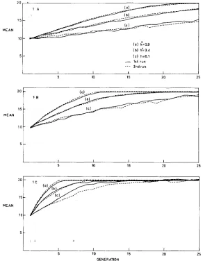
Nine typical pairs of repeated runs are shown in Figure 1 ( L - , B and C)

,

where

(5)

S I M U L A T I O N O F D I R E C T I O N A L S E L E C T I O N 193

were high, though greater when

h'

was low. Even in the latter cases, however, the populations reached a plateau at about the same generation number and at the same maximum possible values. Responses to selection, even in the case of low heritability and tight linkage, were thus not appreciably affected by genetic drift.

Other results were similar and will not be presented.

Predictive value of h2: In experimental work, it is almost impossible to estimate the various parameters in every generation, f o r the accurate prediction of genetic response. Hence it is often assumed that the heritability of a character remains

( 0 1 h1=0.9

I b) h'= 0.4

I C ) h=0.1 - 1st run

2 n d ~ " ...

I I I 1 I I

5 10 15 20 2 5

20 -

1 5 - M E A N

1 0 -

I I I

5 10 15 20 2 5

15

M E A N

1 0

5 10 15 20 25

GENERATION

FIGURE 1 .-Additive model: Replicate runs of nine populations with different recombination probabilities ( r ) and different initial heritabilities ( h z ) under different intensities of selection ( I ) .

(6)

194 S. S. Y. Y O U N G

constant throughout a few generations of selection. Under this assumption, the population mean of the nth generation is predicted by the usual formula as:

n-1

M,= M O

4-

h'

,E,

i j uPj

where

M O

= population mean before selection in the base population (generation 0), M , = population mean of the nth generation, h2 = constant heritability,

i j = average selection differential of parents (in standard units) in the jth

generation, upj = phenotypic standard deviation in the jth generation.

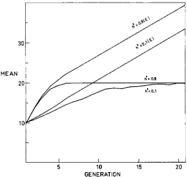
In Figure 2, expected means calculated in this way have been compared with the observed means for each of 20 generations. Two values of h2 (0.9 and 0.1) have been used and one high level of selection intensity ( I = 0.10). As will be shown later, u2.., will in many cases decay rapidly, so that means predicted on the assumption of a constant h' can be expected to be far in excess of means actually realised. Figure 2 clearly demonstrates these discrepancies, which are appreciable even in early generations. When h2 is low, the predictions in the early generations are less accurate than when h2 is high, while at either level of hz the predictions for later generations are meaningless. This conclusion was general among all the results studied, and as the point seems obvious no further data will be presented.

In the present study, it was possible to calculate the heritability and predicted genetic gain f o r each generation, since estimates were available of u Z A , u~~ and the

population means before and after selection. The expected genetic gain of the nth generation plus the unselected population mean in the same generation gave the expected mean of the ( n -t 1)th generation. Comparison of this expected mean with the observed mean of the unselected population at the ( n f 1 ) t h generation provided a comparison of predicted and realised genetic advance.

5 10 15 20

GENERATION

FIGURE 2.-Additive model: Realised advance for hz=0.9 and h2=0.1 and ~ 0 . 0 5 and the

(7)

S I M U L A T I O N O F DIRECTIONAL SELECTION 195

This comparison is valid, since the expected mean at the ( n

4-

1)th generation, calculated from parameters estimated at the nth generation, was quite independent of the unselected population mean at the ( n

+

1 ) th generation, the latter being the result of many random processes including random mating of selected parents and recombination.

Figure 3 compares predicted and realised means for successive generations. Values for

I

= 0.50 and 0.10 have been plotted; those for

I

= 0.80 were similar to those for I = 0.50 and have not been shown. Values for three levels of h' and three of r have been included.

The agreement between the expected and realised genetic advances was close in all cases. However, when a poorly heritable trait was under intense selection the prediction of genetic progress became slightly less accurate. Linkage had, under the present conditions, no apparent effect on the agreement between predicted and realised advance. Under 50% and 10% selection intensities, nearly all populations reached a plateau before 25 generations of selection. With the mild selection intensity of SO%, however, only traits with hz = 0.9 reached a plateau, and then after more than 25 generations of selection. The rate of genetic progress, as expected, is higher when the heritability is high and selection intense. Under 10% selection intensity and high heritability, the populations reached maximum values after 5 to 6 generations of selection, irrespective of the tightness of linkage; in fact, tight linkage tended to accelerate genetic advances in the initial generations.

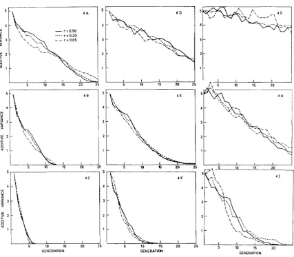
Decay of additive genetic variance: Figure

4

shows the value of u~~ in each generation for each population. The rate of decay was most rapid when selection intensity was high, even for medium levels of heritability. Rates of decay were also affected appreciably by levels of heritability. It is apparent that in situations where selection pressure on the genotypes is high, (that is, with high heritability and/or high selection intensity), the decay curves tend to resemble a negative

exponential type, while under mild pressure they tend to be linear.

In the intense selection set

(I

= 0.10) all except one population reached fixation before 25 generations of selection. In the extreme cases when heritability was high, fixation was reached after only six generations of selection irrespective of linkage values. On the other extreme when h' was very low, mild selection for 30 generations only reduced uZA to a limited extent. Linkage had only small overall effects on the decay of the additive variance. Tight linkage led to a more rapid decay of uZA in the initial generations and had the reverse effect in later generations.

T H E D O M I N A N C E MODEL

I n the present model, genetic values of 2, 2, 0 respectively were assumed for the genotypes 11, 10, and 00. The assumptions used were identical with those used in conjunction with the additive model. Values of uZA were calculated by

(8)

196 S. S. Y. YOUNG

J I I I

D

N : z "

NV3W NV3W

I I I I

(9)

SIMULATION O F DIRECTIONAL SELECTION 197

- 1

\

A C

GENERATION

1-

:.\ 5 10 15 20

4 H

2 -

1 -

I I 1 I ,

10 15 20

4 1

5 10 15 20

GENERATION

FIGURE 4.-Additive model: Decay of the additive genetic variance under different selection intensities ( I ) for populations with different initial heritabilities (hz) and recombination proba- bilities ( r ) . (A) Z=80%, h2=0.90. (B) Z=50%, hZ=0.90. (C) Z=10%, h2=0.90. (D) Z=80%, hz=0.40. (E) Z=50%, hz=0.40. (F) Z=10%, h2=0.40. (G) Z=80% hz=O.lO. (H) Z=50%,

h2=0.10. (I) Z=10%, h2=0.10.

Replicate runs: Agreements between repeated runs were again very close and the results were similar to those obtained under the additive model. Low h2 again led to slight discrepancies between replicates. As these results were not interesting no detailed presentation will be made.

(10)

198 S . S. Y. YOUNG

information has not been presented. In each set of data different values of h2 and

r have been incorporated.

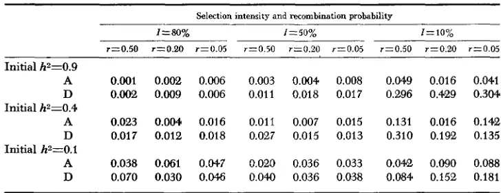
Comparing the present results with those obtained under the additive scheme showed that, in general, the agreement between the estimated and the realised advances under the dominance model were not as good as those under the additive model. The difference in predictability of h2 under the two models can be compared by calculating means and variances of the errors of prediction and these are shown in Tables 1 and 2. Each mean in Table 1 was calculated as the mean of the estimated advance minus the realised advance, so that a positive value indicates a n overestimate while a negative value an underestimate. The calculations were confined to the first 12 generations of selection as differences

TABLE 1

Mean differences between estimated and realised genetic advances (calculated as estimated minus realised)

Selection intensity and recombination probability

]=SO% 1 ~ 5 0 % I=10%

r=0.50 r=O.ZO r z O . 0 5 r=O.50 r=0.20 r=0.05 r z 0 . 5 0 r=0.20 r ~ 0 . 0 5

Initial h2=O.9

A* 0.054 0.012 0.012 0.089 0.040 -0.122 0.187 0.217 0.159 D 4 . 0 6 5 0.184 -0.139 0.207 0.290 0.270 1.668 1.705 1.648 A 4 . 0 5 2 -0.162 -0.018 -0.043 -0.098 -0.201 0.403 0.007 0.118 Initial h2=0.4

D -0.238 -0.167 -0.310 0.081 0.145 -0.010 1.241) 0.772 0.676

Initial h2=0.1

A 0.656 -0.057 0.412 0.216 0.025 -0.061 0.559 0.202 -0.282 D 4 . 0 7 3 -0.178 4 . 0 3 9 0.352 -0.072 -0.008 1.002 0.599 0.738

~ ~ ~~ ~

* A z u n d er the additive model. D=under the dominance model

TABLE 2

Variance of differences between estimated and realised genetic advances

~~ ~ ~

1=80% 1 ~ 5 0 % I=10%

r ~ 0 . 5 0 r x O . 2 0 r z 0 . 0 5 r=0.50 r z 0 . 2 0 r=0.05 r z 0 . 5 0 r = 0 . 2 0 r z 0 . 0 5

Initial h2=0.9

A 0.001 0.002 0.006 0.003 0.004 0.008 0.049 0.016 0.041 D 0.002 0.009 0.006 0.011 0.018 0.017 0.296 0.429 0.3W

A 0.023 0.004 0.016 0.011 0.007 0.015 0.131 0.016 0.142

D 0.017 0.012 0.018 0.027 0.015 0.013 0.310 0.192 0.135 A 0.038 0.061 0.047 0.020 0.036 0.033 0.042 0.090 0.088 D 0.070 0.030 0.046 0.040 0.036 0.038 0.084 0.152 0.181 Initial h2=0.4

Initial h2=0.1

(11)

S I M U L A T I O N O F DIRECTIONAL SELECTION 199 shown in the later generations, resulted mainly from earlier disagreements. This was particularly so for cases under high selection intensities.

Under both models, high intensity of selection coupled with high heritability tended to overestimate genetic advances, while low selection intensity plus low heritability tended to underestimate genetic advances. The trend, however was not pronounced in the additive case but marked and consistent under the dominance model. Under the additive model, where the total advance in some cases covered a range of 10 units, the mean error of prediction was about 2 to 5% of the range. Under the same situations (same combinations of h2 and I ) in the dominance model where the total advance was about five units, a mean error of prediction could be as high as 30% of the range. The relative inaccuracy of prediction under the dominance model is also reflected by its higher error variances shown in Table 2. The higher variance under the dominance model is striking when h' and selection intensity are both high but somewhat less so when h' and Z are intermediate. Under low selection intensity and heritability the variance under both models are similar. Thus the prediction under the dominance model is in general more erratic than under the additive model under majority ofcases inkestigated here. Tightness of linkage again appear to be unimportant in pre- dicting genetic advance.

Under high selection intensity all populations plateaued at the expected maximum value and hence there was no indication of any loss of desirable genes due to fixation of their unfavourable alleles.

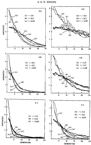
Decay of additiue genetic variance: Figure 6 shows the changes in uZA and uZD

under selection. As the decay was again largely influenced by h2 and I , only the extreme cases (h$ = 0.1, h2 = 0.9) are shown here. The results for h2 = 0.4 were approximately intermediate between the extremes.

In the present model the overall rate of decay in uZA was less rapid than the

additive model. I n cases when h' was high and selection intense the initial rate of decay was still rapid but the remaining portion of uZA tended to remain throughout many generations of selection. Thus when h2 = 0.9, Z = 0.1 about 90% of the total 2 - 4 was lost after four generations of selection, irrespective of the

linkage value, but the remaining 10% was further reduced to zero only after more than ten additional generations of selection. When h2 and selection pressure were both low, the initial rate of decay under the dominance model was faster than under the additive model but the remaining portion of again was reduced only slowly. A fast initial decay and a slow elimination of the remaining portion of o ' ~ tended to be the characteristics of this model.

It can be seen that when h2 was low, changes in uZA and uZD, in time, appeared

to be different for different values of r. However, close examination of the data did not reveal any consistent appreciable effect of linkage on decay rates. The confusion of lines which appear in Figures 6 D, E, and F was almost certainly due to the effect of low heritability on results of selection discussed earlier, for when h2 was high lines for all the r values agreed very well indeed (Figure 6 B, C)

.

(12)

200 S . S . Y. YOUNG

I I

0 9 %

N

NV3W

W

Lo

I I

N

0 P N

I I

0

NV3W

I I

0 Lo

N c

(13)

SIMULATION O F DIRECTIONAL SELECTION 201

than in the case for uZA. In all populations uZD persisted over more than

25

gen-

erations.

DISCUSSION

The use of computers for simulation of genetic systems has two severe limita- tions. Firstly, the genetic models used could probably never mimic the real bio- logical complexities, Secondly, even if a very complex model could be developed, one could never be certain that the results would be applicable to any given real situations. The technique, however, has the obvious advantage of delineating exactly the variables involved in the work, so that unambiguous conclusions can be drawn. I t has also the advantage of allowing experiments to be repeated as many times as warranted.

It

is reasonable therefore to regard studies of this sort as a useful aid in the understanding of selection experiments and in the design of efficient selection plans. With these aims in mind, it is probably unrewarding to use extremely complex genetic models in computer studies, as the results may become too difficult to interpret.

The present results show that, under a simple additive model, if the populations are sufficiently large and if the characters are under the control of many genes, the values of heritability predict genetic gains very well indeed, provided the values are reestimated at intervals. This predictive ability is not appreciably affected by the tightness of linkage or the degree of selection intensity. There is a suggestion that predictions may be slightly less accurate when high selection pressure is applied on a poorly heritable trait, but the discrepancies are small. Under the dominance model, however, prediction is somewhat less accurate when selection pressure is high. When selection pressure is high genetic gains tend to be overestimated and conversely when the pressure is low predictions tend to be slightly underestimated, although under moderate and mild selection pressures prediction of gains is fairly accurate. Again we found no appreciable effects of linkage on prediction.

Contrary to the finding in small populations (FRASER 1957; MARTIN and COCKERHAM 1960), in the additive model tight linkage tends to accelerate genetic advance in the initial generations and only slows down advance in later generations; the overall effect of linkage, however, is small. Also, in the large populations studied here, high selection intensity did not result in the fixation of unfavourable alleles under both the additive and the dominance models as it did in the small populations examined by MARTIN and COCKERHAM ( 1960).

The decay of the additive genetic variance from the maximum value to zero under both models could be very rapid in some cases; for example, under intense selection a trait with a high initial heritability might lose most of its additive genetic variance in under ten generations of selection. At the other extreme, with low heritability and low selection pressure, more than half the variance could still be retained after 30 generations of selection even with the simple additive model.

(14)

202 S. S. Y. YOUNG

4

3 Lo U

2 2

s

1

5 10 15 20 25

t

5 10 15 20 25

( c ) r = 0.05

ln W U

3 3 -

$ 2 2 -

s

1 1 -

I I I I

5 10 15 20 25

( 0 ) r i 0.5

( b ) r = 0.2 ln

0

3 3

w ( c ) r = 0.05

s

; 2 2

1

5 10 15 2 0 2 5

5 10 15 20 25

GENERATION GENERATION

FIGURE 6.-Dominance model: Decay of the additive genetic variance ( ~ 2 ~ ) and the domi-

nance variance ( u z D ) under different selection intensities (I) for populations with different initial heritabilities (h2) and recombnation probabilities ( r ) . (A) I=SO%, h2=0.90. (B) I= 50%’ h2=0.90. (C) Z=lO%, h2=0.90. (D) I=SO%, h2=0.10. (E) Z=50%, h*=0.10. (F) I=

10%’ hZ=O.lO. Broken line: Additive genetic variance; solid line: dominance variance.

(15)

S I M U L A T I O N O F DIRECTIONAL SELECTION 203

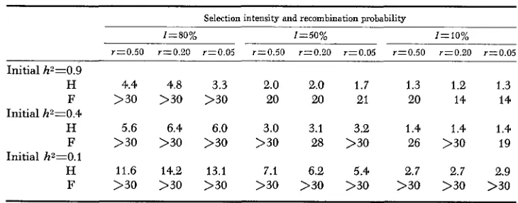
lives" for the additive and dominance models are presented in Tables 3 and

4

respectively, where the fractional generation numbers have been obtained by linear interpolation.

It is apparent from Tables 3 and 4 that changes in selection intensity for the same h2 are always accompanied by changes in the rates of decay. Similarly changes in h* for the same selection intensity are accompanied by changes in the rates of decay. These changes in rates are appreciable. On the other hand changes in the recombination probabilities often have only small or no effect on the rates of decay in genetic variance. Under the additive model tight linkage tends to in-

TABLE 3

Half-life and full-life of the additive genetic variance in different populations under the additive model

I = SO% I=50% I=lO%

r z 0 . 5 0 r r 0 . 2 0 r z 0 . 0 5 r10.50 r=0.20 r=0.05 r=O.50 r=O.ZO r10.05 Initial h*=0.9

H* 9.6 8.9 5.9 3.0 2.9 2.6 1.4 1.6 1.4

F 25.0 27.0 28.0 12.0 12.0 13.0 6.0 6.0 6.0

H 17.9 17.4 16.0 7.0 7.3 6.4 3.1 3.1 2.6

F >30 >30 >30 26.0 30.0 28.0 14.0 13.0 14.0

H 30 30 30 15.7 13.8 16.8 8.2 7.4 5.9

F -

-

- >30 >30 >30 21.0 >30 25.0

Initial h2=0.4

Initial h*=0.1

* Half-life ( H ) =Number of generations of selection required to reduce uzA to one half of its maximum value. Full-life (F) =Number of generations of selection required to reduce mzA to zero.

TABLE 4

Half-life and full-life of the additive genetic variance in different populations under the dominance model

I=50% Z = l O O / ,

r z 0 . 5 0 r=0.20 r=0.05 r x 0 . 5 0 r=0.20 r z 0 . 0 5

Initial h"O.9

H 4.4 4.8 3.3

F >30 >30 >30

H 5.6 6.4 6.0

F >30 >30 >30

H 11.6 14.2 13.1

F >30 >30 >30 Initial h2=0.4

Initial h2=0.1

2.0 2.0 1.7

20 20 21

3.0 3.1 3.2

>30 28 >30

7.1 6.2 5.4

>30 >30 >30

r=0.50 r=0.20

1.3 1.2

20 14

1.4 1.4

26 >30 2.7 2.7 >30 >30

r=0.05 1.3 14 1.4 19 2.9 >30

(16)

204 S. S. Y. YOUNG

crease the initial rate of decay, but later slows down the decrease in uZA, similar

trend under the dominance model, however, is only slight. The varying effect of tight linkage on the decay of uZA seems reasonable, as at the beginning of se-

lection blocks of favourable genes are expected to be favoured by selection and hence lead to a faster decrease in variance; later selection becomes less effective as further reduction of the frequencies of the unfavourable genes must await the incidence of crossing over.

An interesting feature when comparing Tables 3 and 4 is that the half-lives of uZA under the dominance model, in all casse, are appreciably shorter than under the additive model. This is particularly marked when poorly heritable traits are under mild selection pressure. On the other hand the full-lives of the uZA show the reversed situation. This is perhaps expected after the earlier discussion on the results obtained for the dominance model.

I n experimental work with laboratory animals, selection intensities are usually between 10% and 50% while in larger animal work the intensities are usually closer to 50%, if the average intensity for the two parents is considered. I n these cases, under the present models, the half-lives of uZA are short, ranging from only 1 to 7 generations for highly heritable traits and 6 to 17 for poorly heritable traits. Most traits in animals or plants are likely to be controlled by much more complex genetic systems than the one used here. The decay in u Z A is thus likely

to be an overestimate, as it seems reasonable to think that in more complex systems the decrease in u Z A would be slowed down.

Further analyses of the results from the other models used in this series may provide some information on this point.

I n the formulation of breeding plans the level of

h2

determines whether mass selection or family selection is the more efficient system. I n view of the present findings, it seems reasonable to recommend periodic check of heritability after every three to four generations if maximum progress is to be maintained. In this investigation the additive genetic variance, being restricted from the beginning could only decay. The pattern of events found here can be compared with the actual response to selection to assess the importance of decay of additive genetic variance in practice.

This work was done during the tenure of a C.S.I.R.O. Overseas Studentship held at the Biology Department, University of Rochester, N.Y. Grateful acknowledgements are made to PROFESSOR R. C. LEWONTIN (now of the University of Chicago) for his counsel and interest in this investigation and to the Department for the facilities they made available to me. Thanks are also due to MISS E. SMITH for assistance in the tabulation of the results and to MISS H.

NEWTON TURNER and DR. J. M. RENDEL for comments on the manuscript. The costs of computa- tion and publication were borne by U.S. Atomic Energy Commission contracts AT(30-1)-2620 and AT ( 1 1 -1 ) -1 43 7.

SUMMARY

(17)

SIMULATION O F DIRECTIONAL SELECTION 205

eration. Parameters used included 3 levels of selection intensity, 3 levels of heritability, 3 levels of recombination probability and 7 genetic models.

In this paper, the first of a series, the computer programmes are briefly described and the results from the additive and the dominance models presented. Under the additive model, agreements between the realised advances and the expected advances, predicted from the value of heritability and selection differential in each generation, were in most cases very close. Prediction of genetic advances were slightly less accurate when high selection intensity was applied to lowly heritable traits. Linkage had no apparent effect on prediction.

Under the dominance model predictions of genetic advance were less accurate. When selection pressure was high, predictions tended to overestimate genetic advance. On the other hand under low selection pressure, predictions tended to be underestimated. Although in the latter case the agreement between the realised and the expected gains were fairly close.

The decay of the additive genetic variance ( u z A ) under both models was rapid when selection was intense, particularly when heritability was high. By far the most important factors affecting decay were the intensity of selection, and the level of heritability. The effect of linkage on decay was small. I n the additive model, tight linkage tended to accelerate the rate of decay in the initial stages of selection but had the opposite effect in later generations. The same trend was not obvious in the dominance model. The initial rate of decay of u2* was more rapid under the dominance model but later when u~~ was reduced to a low level, the rate of decay under the same model was slower.

I n the large populations studied, no fixation of undesirable alleles, under high selection intensity, was found, and linkage was found to have no appreciable effect on genetic advance.

LITERATURE CITED

BOFINGER, E., and V. J. BOFINGER. 1958 On a periodic property of pseudo-random sequences. J. Assoc. Computing Machinery 5 : 261-265.

CHANG, C. S., and A. B. CHAPMAN, 1958 Comparisons of the predicted and actual gains from selection of parents of inbred progeny of rats. Genetics. 43: 594-600.

CLAYTON, G. A., J. A. MORRIS, and A. ROBERTSON, 1957 An experimental check on quantitative genetical theory. I. Short-term responses to selection .J. Genet. 5 5 : 131-151.

FRASER, A. S. 1957 Simulation of genetic systems by automatic digital computers. I. Introduc- tion. 11. Effects of linkage on rates of advance under selection. Australian J. Biol. Sci 10: 464491, 492-499.

MARTIN, F. G., JR., and C. C. COCKERHAM, 1960 High speed selection studies. pp. 35-45. Bio-

metrical Genetics. Edited by 0 . KEMPTHORNE, Pergamon Press, London.

MARTIN, G. A., and A. E. BELL, 1960 An experimental check on the accuracy of prediction

of response during selection. pp. 178-187. Biometrical Genetics. Edited by 0. KERIPTHORNE, Pergamon Press, London.

Studies in artificial selection of quantitative characters. I. Selection for