Trace Based Performance Characterization and Optimization

(1)

mization. (Under the direction of Associate Professor Frank Mueller).

Processor speeds have increased dramatically in the recent past, but improvement in memory access latencies has not kept pace. As a result, programs that do not make efficient use of the processor caches tend to become increasing memory-bound and do not experience speedups with increasing processor frequency.

In this thesis, we present tools to characterize and optimize the memory access patterns of software programs. Our tools use the program’s memory access trace as a primary input for analysis. Our efforts encompass two broad areas — performance analysis and performance optimization. With performance analysis, our focus is on automating the analysis process as far as possible and on presenting the user with a rich set of metrics, both for single-threaded and multi-threaded programs. With performance optimization, we go one step further and perform automatic transformations based on observed program behavior.

(2)

by

Jaydeep Marathe

A dissertation submitted to the Graduate Faculty of North Carolina State University

in partial fulfillment of the requirements for the Degree of

Doctor of Philosophy

Computer Science

Raleigh,NC 2007

Approved By:

Dr. Yan Solihin Dr. Tao Xie

Dr. Frank Mueller Dr. Vincent Freeh

(3)

Dedication

(4)

Biography

(5)

Acknowledgements

(6)

List of Figures

1.1 Improvement in CPU and DRAM speeds [39] . . . 2

1.2 Comparison of software-based and hardware-based tracing . . . 4

1.3 Our trace-based frameworks . . . 5

2.1 The METRIC Framework [62] . . . 14

2.2 Overall Compression Algorithm . . . 16

2.3 Example RSDs . . . 18

2.4 Example PRSDs . . . 18

2.5 PRSD Detector Flowchart: Processing in a Level [62] . . . 20

2.6 PRSD Detection Example . . . 23

2.7 Execution Time Breakup for Our Compression Scheme, Relative to VPC3 Execution Time . . . 28

2.8 Use of Metrics for Performance Diagnosis . . . 33

2.9 Original Per-Reference Memory Usage Statistics . . . 36

2.10 Evictors for Each Reference . . . 37

2.11 Optimized Per-Reference Memory Usage Statistics . . . 38

2.12 Comparison of L2 Cache Misses . . . 39

2.14 Performance of Original and Optimized Program . . . 43

2.16 Evictor Graph . . . 46

2.17 Optimized Per-Reference Memory Usage Statistics . . . 47

3.1 ccSIM Framework . . . 55

3.2 NBF: Interleaved and Piped . . . 64

3.3 Execution Overhead and Trace Sizes . . . 64

3.4 NBF: Breakdown of L2 misses . . . 68

3.5 IRS: Breakdown of L2 misses . . . 71

3.6 IRS: Time w/ 4 Optimizations . . . 71

3.7 IRS: Per-Reference Statistics . . . 72

3.8 IRS Breakup into Parallel Regions . . . 72

(11)

3.10 SMG: Cumulative L2 Coherence Misses . . . 75

3.11 SMG: Time for different Workloads . . . 75

3.12 Invalidators for Selected References . . . 78

3.13 Reduction in Execution Metrics for AMMP . . . 79

3.14 sPPM, initbuf() in main.m4 . . . 82

3.15 310.wupwise m, rndcnf() in rndcnf.f . . . 82

3.16 FT, compute indexmap in ft.c . . . 82

4.1 Characterization for SMG2000 . . . 92

4.2 Simplified PMU Operation . . . 95

4.3 Comparison of Trace-Based Methods . . . 100

4.4 Characterization using Hardware Performance Counters . . . 106

4.5 Memory Accesses Traced with PMU-based tracing, Normalized to Number of Accesses in Full Trace . . . 107

4.6 Top-10 References Causing Invalidations on Processor 1, PMU Sampling Rates of 1-8 . . . 109

4.7 Top-10 References Resulting in Coherence Misses on Processor 1, PMU Sam-pling Intervals of 1-8, PMU-based tracing . . . 110

4.8 Execution Time: Full-tracing vs. PMU-based tracing . . . 112

4.9 Memory Accesses Traced with Targeted tracing, Normalized to Number of Accesses in Full Trace . . . 113

4.10 Top-10 References Causing Invalidations on Processor 1, Store Sampling Rates of 1,4,10,20 . . . 115

4.11 Top-10 References Resulting in Coherence Misses on Processor 1, Store Sam-pling Rates of 1, 4, 10, 20 . . . 116

4.12 Execution Time: Full-tracingvs. Targeted tracing . . . 117

4.13 Coverage and False Positives for PMU-based and Targeted Tracing with Re-spect to True-sharing Invalidations . . . 118

4.14 Coverage and False Positives for PMU-based and Targeted Tracing with Re-spect to False-Sharing Invalidations . . . 119

4.15 Execution Overhead Comparison . . . 124

5.1 Automatic Profile-guided Page Placement . . . 132

5.2 Simplified PMU Operation . . . 133

5.3 Evaluation with Latency threshold=128, Profile Source=Long Latency Loads 143 5.4 Evaluation with Profile Source=Data TLB Misses . . . 148

6.1 Example Patterns . . . 157

6.2 Overall Framework . . . 160

6.3 Simulator: % Reduction in L1D load misses (Training data set) . . . 166

6.4 H/W: % Reduction in L1D load misses (Reference data set) . . . 167

(12)

List of Tables

2.1 Comparison of Compression Rates . . . 27

3.1 Total L2 invalidations with HPM . . . 62

3.2 HPM vs. ccSIM . . . 62

3.3 NBF: Comparison of per-reference statistics for each optimization strategy . 68 3.4 NBF: Wall clock Times (Seconds) . . . 69

3.5 NBF: L2 Invalidations (HPM raw) . . . 69

3.6 SMG: Per-Reference Statistics (Processor-1) . . . 74

3.7 AMMP: Per-Reference Statistics . . . 77

4.1 Description of Benchmarks . . . 102

4.2 True and False-Sharing Invalidations Caused Measured with Full Traces . . 119

4.3 Ratio of False-Sharing Invalidations to Total Invalidations for the Selected References in PMU Tracing and Full Tracing . . . 122

5.1 Access latencies on the SGI Altix . . . 130

6.1 Benchmarks and data sets . . . 163

(13)

Chapter 1

Introduction

Processor speeds have increased dramatically in the recent past. However, the rate of improvement in DRAM access latencies has been slower, as shown by Figure 1.1. The increasing difference between the performance of the CPU and the memory system has serious implications for contemporary software programs. Another issue is the advent of multicore platforms that are being introduced by all major processor vendors. As the number of cores increase, the demand for memory bandwidth grows, even without increasing the individual processor frequency.

As a result, programs that do not make efficient use of the processor cache will tend to become increasinglymemory boundand will not experience significant speedups with increasing CPU frequency. In fact, programs may even experience performance degradation as the number of cores increases without corresponding increase in memory bandwidth.

(14)

Figure 1.1: Improvement in CPU and DRAM speeds [39]

1.1 Problem Statement

How can a program’s memory trace be used to analyze its behavior and

optimize its performance?

This problem statement has several facets:

1. What are the different methods to obtain the program’s memory access trace?

2. What are the qualityversus overheadtradeoffs between these trace generation meth-ods?

3. What are the different performance analysis and optimization frameworks that are feasible using memory traces?

4. What are the pre-requisites in terms of trace information and detail that these anal-yses entail, and is it possible to satisfy them with memory traces and additional instrumentation?

(15)

1.2 Trace Generation

In our work, we have used memory traces obtained with both software and hard-ware means. In the pure softhard-ware approach, we instrument the memory access instructions of an executing program using dynamic binary instrumentation. Instrumentation at the level of executable instructions enables whole-program trace-based analysis, even for parts of the program for which source code is not available (e.g., third-party libraries). This approach is portable (requires no explicit hardware support) but slows down programs sig-nificantly. Also, the sheer volume of loads and stores, even for programs with small data sets, can be an obstacle for some analyses.

Several processor architectures now have explicit hardware support for extracting memory traces. The Itanium2 and x86 platforms can monitor and capture many load misses. Hardware based tracing has significantly lower overhead (compared to software-based tracing). In addition, the Itanium2 platform allows filtering of loads before capture based on the number of cycles the load took to complete. By setting the filter value appropriately, we can ignore loads that hit in the L1/L2/L3 caches. This vastly reduces the number of loads that are captured and thus also the overhead of the tracing process. We show that many analyses can work effectively with such a filtered trace. On the other hand, current hardware implementations have some restrictions on the memory accesses that can be captured. On contemporary Itanium2 and x86 platforms, hardware limitations make the trace capturelossy,i.e., only a fraction of the qualified trace elements are actually captured. Also, these implementations have no support for capturing store accesses that are essential for some tools (e.g., coherence traffic analysis).

Figures 1.2(a) and 1.2(b) illustrate the tradeoff between hardware and software tracing. The software-based tracer employs binary instrumentation to obtain the load access stream. The hardware-based tracer exploits the Itanium2’s performance monitoring unit to filter out loads taking less than 8 cycles to complete (most L1 and L2 load hits). In addition, the Itanium2 hardware is lossy and drops many of the qualified load samples that should have been captured. We see that the hardware logs about 10 to 100 timesfewer

loads compared to the software tracer, but is more than 10 times faster. In our work, we show that even lossy traces can be effectively used for certain performance analyses and optimizations.

(16)

!" # $%& #' ()*+,

(a) Normalized Execution Time

!"#$%&'(

(b) Normalized # Loads in Trace

Figure 1.2: Comparison of software-based and hardware-based tracing

shown in Figure 1.3. Broadly, our efforts can be divided into automated tools for per-formance evaluation and perper-formance optimization. Frameworks use either software or hardware generated traces or a combination. A brief introduction of the frameworks fol-lows.

1.3 METRIC: Memory hierarchy analysis for single-threaded

benchmarks

The objectives for this work are as follows:

1. To explore the use of memory traces for memory hierarchy performance analysis of single-threaded programs;

2. To explore the use of dynamic binary rewriting for extracting memory traces from an executing program;

3. To test novel light-weight compression strategies for online compression of memory traces;

(17)

Software

Hardware

Performance Optimization uniprocessor programs.

1. METRIC: Cache Analysis for

2. ccSIM: Coherence Traffic Analysis

3. Hybrid H/W−S/W Coherence Analysis

Performance Evaluation

4. Automatic Page Placement for ccNUMA

5. Profile−guided Data Prefetching.

Figure 1.3: Our trace-based frameworks

5. To generate rich metrics that characterize the memory access patterns in the program; and

6. To demonstrate the use of these metrics for effecting novel optimizations that are very hard to achieve with pure static compiler analysis.

We call our tool METRIC (“MEmory TRacIng without re-Compiling”). MET-RIC is a trace-based incremental memory hierarchy simulator that generates a rich set of metrics to aid the analysis of single-threaded programs. The trace consists of memory accesses and scope change events (e.g., enter/exit function) and is obtained via software dynamic binary rewriting of executing programs. The trace is compressed online using a novel compression algorithm. The compressed trace is used offline for incremental memory hierarchy simulation and generates a rich set of metrics tagged to high-level source code constructs like data variables and source locations (line::file).

(18)

1.4 ccSIM: Source-Code Correlated Cache Coherence

Char-acterization of OpenMP Benchmarks

The recent trend towards multi-core and multi-processor shared-memory machines has prompted a shift towards parallel programming. Understanding the sharing of data among threads is essential to detecting and alleviating performance bottlenecks in parallel programs. We explored the use of trace-based analysis for this purpose. The objectives for this work are as follows:

1. To extract traces from multi-threaded OpenMP benchmarks using dynamic binary rewriting, which has not been done before, to the best of our knowledge;

2. To extractsynchronization information among threads, which is essential for correct performance simulation — this entails reverse engineering compiler generated func-tions for OpenMP directives which is unprecedented in past work;

3. To exploit the per-thread memory traces and OpenMP synchronization information for incremental coherence protocol simulation. A unique property of our approach is the ability to relate low-level coherence events such as invalidations to source code constructions such as line::file tuples. In contrast, past work has considered coherence analysis usually from an architecture perspective, instead of the user perspective as we do; and

4. To demonstrate the capability of our framework for detecting, understanding and resolving sharing bottlenecks in large real world programs.

We extended METRIC for analysis of coherence traffic of shared memory mul-tithreaded programs that use OpenMP for parallelism. We call our tool ccSIM (Cache CoherenceSIMulator). We demonstrate that our tool can find optimization opportunities in several production codes that have been used for many years on tens or hundreds of processors.

(19)

1.5 Hybrid Hardware/Software Coherence Analysis

The previous tool (ccSIM) uses software instrumentation to extract the memory access trace. In this work, we explore the use of lossy hardware-generated traces for an-alyzing the coherence traffic at the source code level. The objectives of this work are as follows:

1. To explore the use of the Itanium2 performance monitoring unit (PMU) and high precision timing register to generate filtered memory traces;

2. To measure the execution overhead, trace sizes and degree of lossiness in the PMU-generated trace;

3. To explore software strategies that allow the PMU to trace stores, which it is unable to do natively;

4. To evaluate an alternative software-centric approach that uses high precision timing hardware to filter load instructions in the trace; and

5. To compare and contrast both these methods (PMU-centric, software-centric) with respect to overhead, trace sizes and accuracy of coherence simulation. Accuracy is measured with respect to coherence simulation results achieved with full software tracing (as used in our earlier ccSIM work).

We show that both the PMU-centric and software-centric methods can reduce the number of trace accesses that need to be captured by an order of magnitude while retaining the precision of the corresponding coherence simulation for many benchmarks.

1.6 Hardware Profile-guided Automatic Page Placement for

ccNUMA

(20)

on application performance on ccNUMA machines because remote memory loads are much more expensive compared to loads from local memory. The objectives of this work are as follows:

1. To explore the use of Itanium2 performance monitoring unit to generate traces of filtered long-latency loads for multi-threaded OpenMP programs;

2. To explore the use of these traces for automated page placement without special compiler, linker or operating system support;

3. To support page placement for both static and dynamically allocated regions of mem-ory;

4. To explore the use of an alternative profile source, translation lookaside bufffer (DTLB) misses, for page placement; and

5. To compare and contrast the two profile sources with respect to overhead, quality of the generated page placement and benefits in terms of reduced execution time and remote loads.

1.7 PFetch: Profile-guided Data Prefetching

In contrast to our page placement efforts that tries to reduce the average latency of memory access, we also explored trace-based data prefetching that attempts to hide it instead. The objectives for this work are as follows:

1. To explore the use of memory traces for a novel software-only data prefetching scheme based on observed cross-instruction address predictability;

2. To unify several past approaches that each target a separate source of predictability by introducing a new standard analysis method; and

3. To explore the use of novel threshold-based schemes for addressing the issues of prefetch accuracy, prefetch timeliness and prefetch redundancy.

(21)

we can analyze programs across function, module and library boundaries. In this work, we used our software tracing framework to extract memory access traces from single-threaded programs that exhibit significant cache misses. The traces are analyzed to detect instances ofpredictabilitysuch that the address of a load miss can be predicted given a certain number of previous memory accesses. This predictability can be leveraged to prefetch the missing memory line into cache.

(22)

Chapter 2

METRIC: Memory Tracing Via

Dynamic Binary Rewriting to

Identify Cache Inefficiencies

2.1 Summary

(23)

per-reference metrics, cache evictor information and stream metrics. Finally, we demonstrate how this information can be used to isolate and understand memory access inefficiencies. This illustrates a potential advantage of METRIC over compile-time analysis for sample codes, particularly when interprocedural analysis is required.

2.2 New Contributions

METRIC was first presented in my Master’s thesis [62]. However, since then, we have made significant enhancements to the framework and analysis techniques and also generated new results that supersede the data presented originally. In this chapter, we shall present new results from our enchanced framework. We have explicitly cited the Master’s thesis for parts of the framework that have not changed significantly in the enhanced version — we retain them here to maintain the readability of the text.

We make the following new contributions in this work, compared to the version reported in the Master’s thesis:

• We have re-designed the online compression strategy. The new approach separates compression of trace ordering from trace addresses. We show that our new strategy achieves better compression than the best known state-of-the-art compression schemes for many of the SPEC FP benchmarks.

• We have added new “stream-oriented metrics” to the pre-existing metrics generated by the analysis component.

• We present 3 new use cases for METRIC that would be very hard or impossible to optimize with static compiler analysis.

The following components of METRIC are mostly unchanged from the Master’s thesis version:

• The overall concept of METRIC — using binary instrumentation to extract memory traces, compress them online and use them for offline memory hierarchy simulation.

• The tracing framework based on binary instrumentation.

(24)

• Some metrics generated by the memory hierarchy simulator.

2.3 Introduction

Over the past decade, processor speeds have increased much faster than memory access speeds. Due to this trend, application execution times are increasingly dominated by the time spent in accessing memory. Tools are needed that can efficiently profile the memory access behavior of the program and help in detecting, isolating and understandingcausesof the potential memory access inefficiencies. In this work we present one such tool, METRIC. METRIC employs incremental memory hierarchy simulation using partial memory access traces and generates detailed high-level metrics characterizing the application’s memory use.

Simulation may be performed offline using previously extracted access traces or

online as the application executes. In spite of the accuracy that trace-driven memory simulation affords, efficiency requirements dictate that it be used judiciously. For instance, software tracing incurs high runtime overheads, making full application simulation with reasonable data sets infeasible. Furthermore, even programs with short execution times may generate traces requiring gigabytes of storage. These limitations can be alleviated with partial data traces representing a subset of the access footprint of the target. Such traces tend to be comparatively small and less expensive to collect while still capturing the most critical data access points. Our focus is on scientific benchmarks, which generally employ algorithms with convergence criteria that are checked on a regular basis at the end of atimestep. The computation of each timestep is highly repetitive and, thus, representative for the overall application behavior, as shown elsewhere [108]. Generating and exploiting partial data traces for online incremental memory hierarchy simulation addresses both high tracing overheads and large storage requirements without sacrificing accuracy. This is the approach we take.

(25)

In this work we make the following contributions

• We develop an approach that uses dynamic binary rewriting to extract memory access traces from executing applications.

• We develop a novel algorithm for efficient access trace compression of programs with nested loop structures.

• We present a cache analysis methodology (partially based on prior work by Mellor-Crummey et al. [70]) that uses partial access traces to generate cache metrics — including detailed evictor information — correlated to high-level constructs such as source code locations and data structures.

• We show how METRIC can be used to understand a diverse range of memory access inefficiencies, some of which are hard to detect with static compiler analysis.

METRIC builds on the DynInst instrumentation framework [10] to exploit dy-namic binary rewriting, or post link time manipulation of binary executables, enabling program transformation potentially even while the target is executing. Unlike conventional instrumentation, which generally requires compiler interaction (e.g., for profiling) or inclu-sion of special libraries (e.g., for heap monitoring), this approach obviates requirements of recompiling or relinking.

Dynamic binary rewriting can capture memory references of the entire applica-tion, including library routines, and it works equally well for mixed language applications commonly found in production scientific codes [108]. The techniques can be adapted to address changing input dependencies and application modes,i.e., changes over time in ap-plication behavior. Furthermore, binary manipulation techniques have been shown to offer new opportunities for program transformations, and these potentially yield performance gains beyond the scope of static code optimization without profile guided feedback [5].

2.4 The METRIC Framework

(26)

Handler() Handler() Handler() _Trace Variable MHSim OFFLINE Executing Allow Target 3 2 5 6 7 Information Scope Information Information Access pt. <line,file> tuples Points of Interest Module Compression Trace Compressed Driver _Simulator Statistics Cache Detailed Human Compressed Trace Output Shared Object Target to continue about target Extrace information Generation Trace 4 1 Correlation Trace Feedback User ONLINE insert snippet Attach to Target &

Controller

Figure 2.1: The METRIC Framework [62]

executables. To achieve this, we dynamically modify the executing application by injecting instrumentation code via binary rewriting. We instrument memory access instructions to precisely capture the data access stream of the target application, and the user may activate or deactivate tracing so that data reference streams are selectively generated. This facility builds the foundation for capturing partial memory traces.

Figure 2.1 shows two phases in the process of analyzing bottlenecks with METRIC — online and offline. In the online phase, we instrument the application and extract the memory access trace. After trace generation is complete, the instrumentation is removed and the target application continues its execution without overhead. The traces are then used offline for memory hierarchy simulation in a background process or on a separate processor.

(27)

target application’s source code. The instrumentation consists of calls to handler functions in a shared library. The shared library is loaded into the target’s address space through a special one-shot instrumentation.

Once instrumentation is complete, the target is allowed to continue. As the instru-mented application executes, different handler functions in the shared library get invoked, depending on the type of event being recorded,i.e., load, store, enter scope and exit scope. The handler functions, in turn, call the compression routines, which attempt to detect reg-ular patterns in the incoming stream. The compression routines maintain statistics about the regularity of the access stream seen at each memory access instruction. These metrics are presented to the user along with the memory access metrics generated by the memory simulator (in the next step).

After a specified number of events has been logged or a time threshold has been reached, instrumentation is removed and the target continues executing without overhead. The compressed partial event trace is then used offline for incremental cache simulation. The cache simulator driver reverse maps addresses to variables in the source, using infor-mation extracted by the controller program, and it tags accesses to source code locations (source filename::line number). In addition to summary level information, the cache simu-lator generates detailed evictor information for source-related data structures. This infor-mation is presented to the user, along with the per-reference regularity metrics calculated by the compression algorithm.

For relating memory statistics to source code, we exploit source-related debugging information embedded in binaries. The application must provide the symbolic information in the binary (e.g., generally by using the-gflag when compiling). Most modern compilers allow inclusion of symbolic information even if compiling with full optimizations (gcc and xlc on our platform).

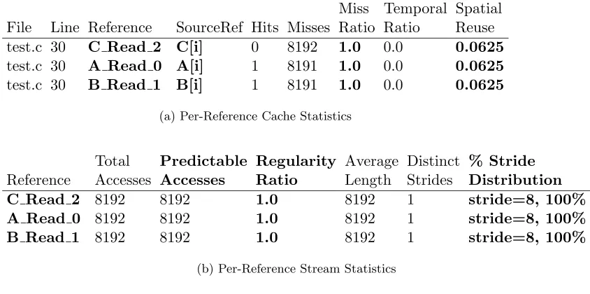
2.5 Trace Generation and Compression

(28)

<Point_ID, EA>

PRSD Detector

LibBZIP

Regular Irregular

Accesses Accesses Predictable Address ?

NO YES

Trace.PC

Memory Access Stream

Ordering

Access Pattern SEQUITUR

LibBZIP

Compressed _{Compressed Access Stream} Regularity

Metrics

Figure 2.2: Overall Compression Algorithm

access point. These metrics provide key information during the analysis phase.

With this work we target scientific applications that tend to have highly regular accesses, usually in nested loops. We tailor our compression algorithm for this scenario. Our compression strategy is shown in Figure 2.2. The access stream to be compressed consists of individual records described by the tuple <point id, EA>. Point id denotes the access instruction andEA is the data address generated by the instruction. The task of compression is split into two parts. Theorderingamong the different access instructions is compressed separately from thedata addressgenerated by the individual access instructions. The idea is to use different compression algorithms suited to these distinct tasks to achieve more effective compression. It is necessary to record the access ordering for correct memory hierarchy simulation during the later phases.

2.5.1 Compressing Access Ordering

(29)

SEQUITUR is described by Nevill-Manning and Witten [78]. It converts a trace of symbols into a context-free grammar, and has time overhead linear in the number of symbols in the trace [79]. The expansion of the grammar can be used to regenerate the original trace. SEQUITUR requires memory proportional to the total number of symbols occurring in the grammar. Since the total number of unique instruction addresses in the trace is usually small compared to the total program size, SEQUITUR is well suited for our purpose. We have observed extremely high compression rates with SEQUITUR on the SPEC2K FP benchmarks. In addition, decompression can proceedincrementally,i.e., compressed traces can be used directly for cache simulation without an intermediate trace expansion step.

2.5.2 Compressing Trace Accesses

The accesses generated by each access point, i.e., the data addresses of memory references, are compressed separately. In other words, our compression scheme exploits the

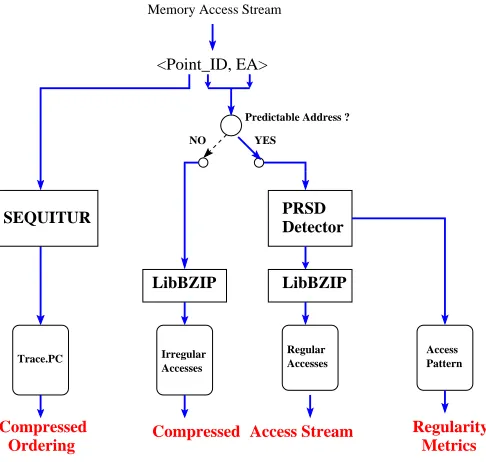
localvalue locality of each access point. The compression algorithm is tailored for regular ac-cesses generated by tightly nested loops. The basic unit of representation for the compressed stream is theregular section descriptor(RSD), an extension of Havlak and Kennedy’s RSDs [38]. Each RSD is a tuple<point id, start address, length, address stride>. Intuitively, each RSD compactly represents a stream of regular accesses generated at a given access point. The point id is the access point generating this RSD. The start address denotes the starting address of the stream, the length indicates the number of accesses in the RSD. The address stride denotes the change in addresses between successive addresses in the RSD. The stride of RSDs may be an arbitrary function. We restrict ourselves to constants in this work since we require fast online techniques to recognize RSDs. In different contexts, one may want to consider linear functions or higher order polynomials. Recurring references to a scalar or to the same array element map to RSDs with a constant address stride of zero. An example RSD is shown in Figure 2.3, assuming each array element has size one.

RSDs are only sufficient to describe accesses generated by a single innermost loop. In order to efficiently describe accesses by a nest of loops, we introduce the power regular section descriptor (PRSD). A PRSD is described by the tuple <point id, start address, length, address stride, child RSD>. A PRSD is similar to an RSD, but instead of generating

(30)

A[i] = B[2i+2] + C[5i];

For ( I = 0; I < N; I++)

{

}

Generated RSDs

RSD_1 < 1, &A[0], N, 1>

RSD_3< 3, &C[0], N, 5>

RSD_2< 2, &B[2], N, 2>

RSD< access_point, start_address, length, address_stride>

Program Code

Figure 2.3: Example RSDs

RSD < 1, &A[0][0], M, 1> RSD < 1, &A[1][0], M, 1> RSD < 1, &A[2][0], M, 1>

RSD < 2, &B[1][1], M, 1> RSD < 2, &B[2][1], M, 1>

RSD < 2, &B[N][1], M, 1>

< 1,start_addr, M, 1>

PRSD < 2, &B[1][1], N, 200, RSD_2>

< 2,start_addr, M, 1> RSDs of A[I][J]

{

For ( j = 0; j < M; j++)

}

For ( i = 0; i < N; i++)

Generated PRSDs

RSDs of B[I+1][J+1]

Generated RSDs

PRSDs of A[I][J]

PRSD < 1, &A[0][0], N, 200, RSD_1>

PRSDs of B[I+1][J+1] , M, 1>

RSD < 1, &A[N−1][0] int A[200][200], B[200][200];

PRSD<point_id, start_addr, length, stride, PRSD/RSD> RSD<point_id, start_addr, length, stride>

A[i][j] = B[i+1][j+1]

Program Code

Figure 2.4: Example PRSDs

PRSD/RSDs. Thus the recursive structures of the PRSD allows efficient representation of regular accesses generated in tight loop nests.

(31)

Each instance of the PRSD is an RSD that has M elements and an address stride of one. This RSD describes all iterations in the inner j loop. The compression of data accesses proceeds as follows. The PRSD detector checks whether the incoming data access is predictable by a PRSD/RSD. If the access is predictable, the PRSD/RSD data structures are updated. Accesses may cause evictions of currently existing PRSDs/RSDs (as described in the next section). These evicted PRSDs/RSDs are further compressed by a second stage compressor based on the open source BZIP2 package [94]. BZIP2 compresses using a block sorting algorithm described by Burrows and Wheeler [15].

RSDs with less than three elements are considered irregular accesses. Irregular accesses are compressed by a separate instance of the BZIP2-based second stage compressor. In addition to compression, the PRSD detector also computes metrics characterizing the regularity of the data accesses generated by each access point. These metrics are presented in later sections and help in deeper understanding of the program’s memory access behavior.

2.6 Online Detection of PRSDs and RSDs

In this section we introduce our algorithm for efficient detection of PRSDs and RSDs from the data access stream generated at each access point. To simplify the notation, we consider RSDs to be a special instance of PRSDs in the description of the algorithm. Theheightof the PRSD denotes the number of child RSDs encapsulated by the PRSD, and indicates the degree of hierarchy of the PRSD. RSDs have height zero (since they themselves do not have child RSDs).

The overall algorithm has been previously described in my Master’s thesis [62]. However, we have modified that algorithm to only compress the trace addresses and not the traceordering. The ordering is now compressed separately by SEQUITUR. As a result, we have removed the concept of explicit sequencing (sequence values and strides) from the original algorithm. In addition, the description has been revamped for readability.

The algorithm is intuitive. The algorithm builds up hierarchical structures (i.e.,

(32)

Start

Element(X)Incoming Retrieve

No

Yes

Increment

End Yes

No

child(X) ? PRSD length Form new PRSD

is_compatible_ sibling(X) ?

Flush

All Levels >= this level

End

Yes

No

Yes Yes

End

State=Empty

Store X.

State=Single

State=Compound

End

Condition Output Error

No

Push Current Element

State=Empty

to next level or flush if MAXLEVEL

State=Compound ? State=Single ? State=Empty ?

is_compatible_

Figure 2.5: PRSD Detector Flowchart: Processing in a Level [62]

triggers formation of a new PRSD, and potentiallyflushesthe current PRSD to the output buffer.

2.6.1 Levels

(33)

Each level is always in one of three states — empty,single or compound. A level in state empty has no PRSDs. Similarly, a level in state single has only a single PRSD. A level in statecompound has a composite PRSD. The idea is that an incoming PRSD at this level would be checked against the composite PRSD to see if it qualifies as a “child” of the composite PRSD. If so, we only need to increment the length of the composite PRSD by one — the incoming PRSD was expected. For streams with long regular accesses, we expect the level to be in the compoundstate for long stretches of processing.

2.6.2 Per-level Processing

Figure 2.5 shows the processing at each level. All levels are initially empty. Let

X denote the incoming element to be processed at the current level number. As described earlier, the data access to be compressed is processed at level zero. Thus, X for level zero will be simply a data address. At higher-numbered levels, Xwill be a PRSD.

The processing of X is determined by the current state of the level. If the level is empty, the incoming element is simply stored, the level state is changed to single and processing ends.

If the level is in state single, there already exists a PRSD “Y” at this level. We try to combine the incoming elementX with the current element Yto form a more deeply nested PRSD with a height equal to the height of Y plus one. This checking is done by the function is compatible sibling. Two PRSDs are compatible if they have the same height, length and their children are also compatible with each other (checked recursively by is compatible sibling). If the elements are compatible, a new PRSD (“composite PRSD”) is formed with length two and a height equal to the height of Y plus one. This new PRSD will have the start address same as the start address ofYand an address stride of the difference between the start addresses of Y and X, and it will encapsulate Y as the child prsd.

If X and Y are not compatible siblings, a change in the data access pattern is detected, e.g., caused by a phase change in the program. We then flush all PRSDs in the current and higher-numbered levels, reset the level state to empty and resume processing. In this manner, phase changes are gracefully detected and handled.

(34)

this PRSD. This check is performed by the is compatible child function. The function first checks ifXis a compatible sibling of thechildrenofY, using theis compatible sibling function introduced before. Next, the function checks if the start address of X is equal to Y.start address + Y.length * Y.address stride, i.e., if X is the next instance of the PRSDs produced byY. Ifis compatible childsucceeds, we simply increment the length ofYand processing ends.

IfXis not a compatible child ofY, we pushYto the next level (where it is processed according to the flowchart), reset the level state to empty, and restart processing at this level with X again. The idea is that with future accesses, X might form a new PRSD Z that is compatible with Y. Z will be compared to Y when Z is pushed to the next level (If this new PRSD Z is still incompatible with Y, the flowchart illustrates that this will cause Y to be flushed). With access points in a recursive function, the number of levels is potentially unbounded. To guard against this, we specify a MAXLEVEL constant value beyond which the element being pushed is simply flushed to the output buffer, rather than being re-processed at a higher level.

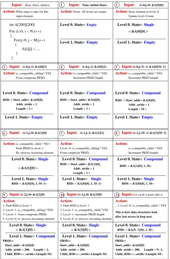
2.6.3 Example

Figure 2.6 shows the operation of the PRSD detection algorithm for the A[i][j] reference shown in Figure 2.4. The figure shows the accesses generated at different instances of the loop nest, the expected actions that the algorithm executes, and the state of the data structures after these actions.

Let us step through some of the frames in the example. For each frame, we show the value of the loop index variablesiandjand the corresponding memory address generated, which is input to the PRSD detection algorithm.

Frame 1: This shows the initial state. All the levels are in stateempty.

Frame 2: (i=0, j=0, &A[0][0]): This is the first iteration point in the loop nest. The incoming element is stored in level zero and the state of the level is changed to single. Frame 3: (i=0, j=1, &A[0][1]): The incoming element and the resident element are compared to verify that they can be combined into a composite PRSD

(is compatible sibling). The new composite PRSD has length two, and the state of the level is updated to compound.

(35)

3 4 5 7 6 9 10 8 1 2 11

is_compatible_child ? YES

Increment PRSD length. Increment PRSD length.

Action:is_compatible_child ? YES Form composite PRSD.

is_compatible_sibling? YES Action: Action:

RSD: < Start_addr= &A[0][0], Addr_stride = 1 Length = 2 >

RSD: < Start_addr= &A[0][0], Addr_stride = 1 Length = M > Level 0. State= Level 0. State=

Level 0. State=Compound Compound Compound

Level 1. State=Empty Level 1. State=Empty Empty

Level 1. State=

Action:None. All levels are empty.

Action:What steps to take for this input element.

Action:Store element in level−0. Update level−0 state

Action:is_compatible_child ? NO ! Push PRSD to level−1. Re−process incoming element

Action:

Level−0: is_compatible_sibling? YES Form composite PRSD.

Action:

is_compatible_child ? YES Increment PRSD length.

Action: Action:

1. Push RSD to level−1

2. Level−1: is_compatible_sibling? YES 3. Level−1: Form composite PRSD 4. Level−0: re−process incoming element

1. Push RSD to level−1 3. Level−1: increment PRSD length 2. Level−1: is_compatible_child? YES

Action:

1. Level−0: is_compatible_child ? YES

after last access in loop nest. This is how data structures look

4. Level−0: re−process incoming element

Level 0. State=Compound Single

Level 0. State= Single

Level 0. State=

< &A[2][0] > < &A[3][0] > RSD: < &A[N−1][0], 1, M> Level 1. State=Compound Compound

Level 1. State= Compound

Level 1. State= PRSD:<

Addr_stride = 200, Length = 2, Child_RSD=<−,stride=1,length=M>

PRSD:< Start_addr= &A[0][0]

Child_RSD=<−,stride=1,length=M> Addr_stride = 200,

Start_addr= &A[0][0]

PRSD:<

Child_RSD=<−,stride=1,length=M> Start_addr= &A[0][0]

Addr_stride = 200, Length = N−1, A[i][j] = ....

} } {

For(j=0; j < M;j++) {

For (i=0; i < N;i++) int A[200][200]

Input: Input: None (initial State) Input:

Input:

(Iiter, Jiter), address (i=0,j=0) &A[0][0]

(i=0,j=2) &A[0][2] Input:

Input:

(i=0,j=N−1) &A[0][M−1]

Input: Input: (i=0,j=1) &A[0][1]

< &A[1][0] >

Level 0. State=Compound Level 0. State=Compound RSD: < &A[1][0], 1, M> Single

Level 0. State=

Level 1. State=Single RSD: < &A[0][0], 1, M> Level 1. State= Single

Level 1. State=Single

RSD: < &A[0][0], 1, M−1> RSD: < &A[0][0], 1, M−1>

Input: (i=1,j=1) &A[1][1]

Input: (i=1,j=0) &A[1][0]

Input:(i=2,j=0) &A[2][0] Input:(i=3,j=0) &A[3][0]

(i=1,j=M−1) &A[1][M−1] Level 0. State=

Level 1. State= Level 0. State=

Level 1. State=

< &A[0][0] >

Empty

Single

Empty

(i=N−1,j=M−1) &A[N−1][M−1]

(36)

it can be considered to be achild of the currently resident composite PRSD

(is compatible child). The length of the composite PRSD is incremented by one and processing ends.

Now we skip to the last iteration of the i loop in the same iteration of the i loop. Frame 5: (i=0, j=M-1, &A[0][M-1]): The incoming element qualifies as a child of the resident PRSD (is compatible child).The length of the resident PRSD is incremented by one and processing ends.

Frame 6: (i=1, j=0, &A[1][0]): This is the very next iteration point of the loop nest after Frame 5 and is the first access in iteration 1 of the i loop. AssumingMis smaller than 200 (the lower dimension of the array), the currently resident PRSD will not correctly predict the incoming element (the PRSD will predict address &A[0][M+1], the incoming address is &A[1][0]), i.e., is compatible child will fail. The currently resident PRSD is pushed to the next level, and the incoming element is saved in the current level.

Frame 9: (i=2, j=0, &A[2][0]): This is the next iteration point after Frame 8. The incoming element will not be predicted by the currently resident PRSD on level zero (similar to Frame 6), which will cause the PRSD to be pushed to the next level (level one). In level one, this PRSD is compared to the pre-resident PRSD to verify that they are compatible siblings (is compatible sibling), after which a new composite PRSD is formed with length two, as shown. The state of level zero is reset toemptyand processing is restarted with the incoming address &A[2][0].

Frame 10: (i=3, j=0, &A[3][0]): Similar to Frame 9, the resident PRSD at level zero will not be able to predict the incoming address &A[3][0]. This will cause the resident PRSD to be pushed upwards to level one, where it will qualify as a child of the pre-resident PRSD. This will cause the length of the pre-resident PRSD at level one to be incremented by one, as shown.

(37)

2.6.4 Space Complexity

In the worst case, a completely random sequence of addresses can be passed to the PRSD detection algorithm. In this case, no RSDs or PRSDs will be detected and the accesses will be recorded individually as irregular accesses. Thus, the space complexity of the algorithm is O(M), whereMis the total number of accesses (i.e., linear space complexity). The best case input is a stream of regular accesses. For such input the algorithm would, at best, generate exactly one PRSD for each access point. The space required to represent a PRSD is proportional to its height. The height of the PRSD in a particular level can be at most one greater than the level number, which has an upper bound given by the constant value MAXLEVELS. Thus, the space complexity to represent the PRSDs for n access points is bounded as O((MAXLEVELS+1)*n). n is an attribute of the source code and is constant for the duration of monitoring. Since both factors are constant, the best case space complexity has a constant upper bound.

2.6.5 Time Complexity

Since we must look at each incoming element to compress it, the lower bound on the time complexity is given as Ω(M), where M is the total number of accesses in the trace. A particular incoming access may trigger movement of PRSDs/RSDs to higher-numbered levels, where they need to be re-processed. The number of re-processing steps is bounded by the maximum number of levels (MAXLEVELS) and the height of the PRSD, which can be at most (MAXLEVELS+1). Thus, the upper bound on time complexity is O(M*MAXLEVELS*MAXLEVELS). Since MAXLEVELS is constant, the upper bound on the time complexity is linear in the number of accesses in the trace.

2.7 Evaluation of the Compression Scheme

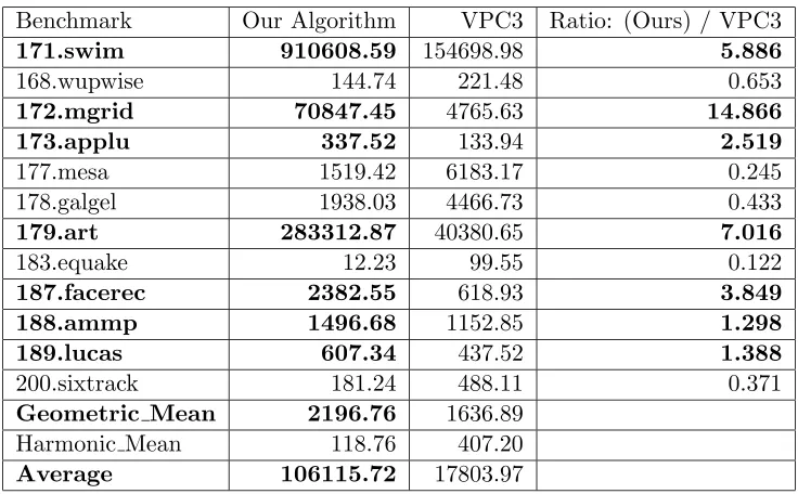
In this section, we evaluate the performance of our compression scheme with re-spect to compression efficiency and time required for compression. We compare our results for 12 out of the 14 SPEC2000FP benchmarks 1

. Results are compared against VPC3, a

1

(38)

state-of-the-art compression algorithm based on using value predictors for data compression [16].

2.7.1 VPC3

VPC3 is targeted for compression of extended address traces. Such traces contain the instruction address (PC) of the access instruction, followed by one or more register values or effective addresses (EA). VPC3 first splits the access stream into separate streams of PCs and EAs. The algorithm has a bank of value predictors that attempt to predict the target element value (PC or EA). All predictors are updated after each element has been processed. VPC3 by itself does not compress the trace. Instead, it writes out the id of the value predictor that successfully predicted the current element. This stream of ids is compressed by a second stage compressor based on BZIP2. Elements that were not predicted by any predictor are compressed by a separate instance of the second stage compressor. In our experiments, we use the VPC3 source code obtained from the author’s website [17] and couple the output to a second stage compressor based on BZIP2 [94].

We use VPC3 for comparison since it represents the state-of-the-art in compressing access traces. VPC3 has been shown to compress faster and with more effective compres-sion rate for most benchmarks, compared to several contemporary comprescompres-sion algorithms (SEQUITUR, BZIP2, GZIP) [16]. VPC3 is targeted towards efficiently compressing the address traces of general purpose programs while we focus specifically on programs found in scientific computing. However, in addition to compressing access traces, our approach generates metrics that characterize the address stream (described later in Section 2.11). These metrics, along with the results generated by the simulator, provide insight into the application’s memory access behavior.

2.7.2 Experimental Setup

For our compression scheme we used the open source implementation of SE-QUITUR [61]. All benchmarks were compiled at -O2 optimization level on an IBM POWER4 platform. All benchmarks used “training” data sets. The static call graph of the target program was traversed with main as root, and all memory access points in the call graph were instrumented. Up to one billion (109

(39)

on-Table 2.1: Comparison of Compression Rates

Benchmark Our Algorithm VPC3 Ratio: (Ours) / VPC3

171.swim 910608.59 154698.98 5.886

168.wupwise 144.74 221.48 0.653

172.mgrid 70847.45 4765.63 14.866

173.applu 337.52 133.94 2.519

177.mesa 1519.42 6183.17 0.245

178.galgel 1938.03 4466.73 0.433

179.art 283312.87 40380.65 7.016

183.equake 12.23 99.55 0.122

187.facerec 2382.55 618.93 3.849

188.ammp 1496.68 1152.85 1.298

189.lucas 607.34 437.52 1.388

200.sixtrack 181.24 488.11 0.371

Geometric Mean 2196.76 1636.89

Harmonic Mean 118.76 407.20

Average 106115.72 17803.97

line for each benchmark. All benchmarks reached the one billion limit, except for 177.mesa (8x106

total accesses) and 188.ammp (531x106

total accesses).

2.7.3 Comparison of Compression Rates

The compression rate was computed as follows. The uncompressed access trace is composed of <point id, address>records. Each uncompressed record requires six bytes — four bytes for the 32-bit address and two bytes for the point id. Notice that all our programs had less than 65536 memory access points. Thus the total uncompressed trace size is (# total records) * 6. The compression rate is calculated as size of un−compressed trace

size of compressed trace .

(40)

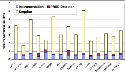
Figure 2.7: Execution Time Breakup for Our Compression Scheme, Relative to VPC3 Execution Time

about 25% greater than the value for VPC3.

2.7.4 Comparison of Compression Times

Figure 2.7 shows the time required for compression using our algorithm. The time for three different components is shown. Instrumentation denotes the overhead of the bi-nary instrumentation framework (e.g., saving/restoring register context). PRSD Detector

(41)

com-pression capabilities on programs where the accesses are less regular. However, we would lose structural information inherent to PRSDs after BZIP compression. Nevertheless, the PRSD predictor would still generate theregularitymetrics (discussed later in Section 2.11) that complement the results generated by the memory hierarchy simulator. Finally, we note that METRIC is capable of and intended for gatheringpartialaccess traces, where the overhead of trace compression is limited by the duration of monitoring. Thus, in practice, a slightly more expensive scheme might still be acceptable as long as the trace collection period is short.

2.8 Memory Hierarchy Simulation

The compressed trace obtained in the preceding sections is used offline for incre-mental memory hierarchy simulation. After a partial trace of accesses has been collected, the instrumentation is removed dynamically and the application continues execution with-out overhead. For programs that exhibit distinct phases of execution (e.g., time-stepped programs), this allows us to limit the overhead of performance analysis by capturing and simulating only “snippets” of the complete trace.

For memory hierarchy simulation, we use a modified version of MHSim [70]. MH-Sim simulates the data TLB (translation Lookaside Buffer) and multiple levels of cache. MHSim maintains information per-reference, allowing “bulk metrics” regarding memory performance (e.g., hits, misses) to be drilled down and mapped to individual access points. For each access point, it generates a rich set of metrics that we shall discuss further below. The original MHSim package used a source-to-source Fortran translator to annotate data accesses with calls to MHSim cache simulation routines. This strategy has two significant disadvantages, which we overcome with our approach.

(42)

references). Thus, the resultant executable with instrumentation can be totally different (in terms of memory access patterns) from the original uninstrumented version — which can lead to potentially misleading diagnostic information reported by MHSim. In contrast, by instrumenting the final optimized binary generated by the compiler, we guarantee that we still capture the exact original access pattern. Thus, we can generate diagnostic information that correctly reflects the target program behavior. Consequently, we argue that source-level instrumentation is the wrong abstraction level for capturing the original application behavior and can lead to potentially misleading results for programs in our target domain (loop-oriented scientific codes).

The second major problem with source-level instrumentation frameworks is that they are limited to a particular language. Many scientific programs are mixed-language ap-plications [108]. In addition, many programs make heavy use of libraries (e.g., Standard C library (libc), math and numerical libraries, networking libraries), that a source level instru-mentation frameworks will be unable to instrument. Thus the resultant trace of memory accesses may be incomplete and can lead to potentially misleading diagnostic information. In contrast, our approach is independent of any language, compiler and linker. More impor-tantly, we usedynamicbinary rewriting that allows us to instrument target applications as they are executing. Thus, we can turn the instrumentation on and off, enabling the capture of partial access traces as discussed before. The resulting overhead of trace collection and instrumentation is flexible and is only limited to the duration of monitoring.

2.9 Abstracting Trace Data

(43)

allows us to reverse map accesses to function-local variables. Finally, dynamically allocated variables can be partially supported by instrumenting the entry to allocation functions (malloc/calloc/free) and walking the call stack at allocation to create a unique “allocation context” identifier. The data accesses to elements in the dynamically allocated area will be reverse mapped and tagged to this identifier in the MHSim report.

2.10 MHSim-generated Metrics

MHSim generates metrics for each level of cache and also for the data TLB. Metrics can be aggregated by reference, by variable and by loop nest. We shall list and describe each metric and later discuss their value as diagnostic input to understand memory behavior. MHSim generates the following metrics per-reference:

• Hits: Number of accesses by this reference point that hit in the cache.

• Misses: Number of accesses by this reference point that missed in the cache.

• Miss Ratio Ratio of hits to misses.

• Temporal Hit Fraction: The fraction of the hits that occurred due totemporal reuse

of data. Calculated as temporal hits_{total hits} . MHSim uses bit vectors to maintain information about which byte offsets in the cache line were addressed by access instructions, allow-ing classification of hits into temporal and non-temporal hits. Temporal hits include hits caused by bothself-reuse(same reference point accesses a memory location mul-tiple times) andcross-reuse(different reference points access same memory location).

• Spatial Hit Fraction: This is defined as 1 - temporal hit fraction,i.e., non-temporal hits are classified as purely spatial hits.

• Spatial Reuse: This value gives the average fraction of the memory line in bytes that wasused,i.e., explicitly addressed by a memory access instruction, before the memory line was evicted from the cache. It is computed as _{cache line size}used bytes

∗number of evictions.

(44)

2.11 Stream-oriented Metrics

In addition to the metrics generated by MHSim, the PRSD detector in the com-pression algorithm also generates complementary metrics characterizing the regularity of the access stream. These metrics are calculated separately for each access point. The following metrics are generated:

• Regularity ratio: Computed as _{total accesses at this point}total predictable accesses . Predictable accesses are those detected as an instance of an RSD or PRSD. The regularity ratio allows us to classify access points into irregular and regular categories. Access points with high regularity ratios can be targeted for stream-based optimizations, as described in our previous work [71]. For example, the predictable nature of the access point can be exploited by prefetching, which caches future data access early to lessen effective access latencies.

• Mean stream length: The average of the length of all RSDs generated at this point.

• # Distinct lengths: Number of distinct RSD lengths seen at this access point.

• % Distribution of distinct lengths: The distribution of RSDs according to their lengths.

• # Distinct strides: Number of address strides for all RSDs seen at this point.

• % Distribution of distinct strides: The distribution of RSDs according to their address strides.

(45)

Metric Diagnostic Information

Miss Ratio A basic measure of performance. References with high or medium miss ratios should be specifically singled out for further analysis. A high miss ratio, when other indicators like regularity ratio and stream lengths have favorable values, indicates presence of specific cache access inefficiencies.

Temporal Hit Fraction

This measures how much temporal reuse is being realized for the memory lines accessed by this reference. Low value may indicate that the reference is being flushed from cache before reuse could occur. If low temporal reuse is inherent to the reference,cache hintingcan be used to avoid allocating a cache line (this requires other indicators to show specific behavior, see text for use case).

Spatial Reuse Low values indicate that cache is not being used efficiently — data is being brought in which is never “touched” before the memory line is evicted from cache. Can indicate presence of conflict misses, if regularity metrics (regularity ratio, stride values) show regular and low-strided access behavior.

Evictor Refer-ences

A cycle of evictors coupled with other indicators like low spatial reuse can indicate presence of conflict misses. The advantage of evictor references is that it tells us precisely which references are involved in the conflict, allowing straightforward code/data transformations to correct it. On the other hand, when other indicators of cache efficiency (e.g., spatial reuse) are high, cycles of evictors may still indicate the presence ofcapacitymisses — there is simply not enough room in the cache to keep all the accessed data at the same time. Regularity

ra-tio

Highly regular streams produce predictablevalues, which can be ex-ploited by optimizations like prefetching. On the other hand, irreg-ular references can be optimized by another class of optimizations (e.g., cache hinting). References with high regularity ratios that still have high miss rates reveal the presence of cache access inefficiencies.

Mean stream

length

Optimizations like prefetching require a minimum stream length to be profitable.

% Distribution of strides

Low-strided references should be expected to have high spatial reuse values, otherwise a cache access inefficiency is indicated. If there are only a few dominant strides, it may simplify the implementation of optimizations like prefetching (knowing dominant stride value allows manual insertion of prefetch instructions without depending on the compiler.)

(46)

2.12 Diagnosis of Performance Problems

In previous paragraphs, we introduced several metrics to quantify different facets of memory access performance. What diagnostic information do these metrics provide? How can we use them to understand the symptoms and the underlying causes of memory access inefficiencies? Figure 2.8 gives a short overview of how the generated metrics can be used for this task.

METRIC gives insight on the memory access patterns of the target program. The information provided by METRIC allows the program analyst to focus on the bottleneck of the program, and also gives indications on how a bottleneck can be removed by manually applying program or data transformations. Many of these transformations can also be achieved by contemporary compiler technology. Such transformations were presented in our earlier work for some well known computation kernels [65]. This work will not reiterate them. Instead, we shall use METRIC to optimize several sample codes to illustrate its potential advantage over compile-time analysis, particularly when interprocedural analysis is required. For clarity of presentation, the sample codes are microbenchmarks that manifest a particular performance weakness. They represent behavior that can arise in larger real world programs.

2.12.1 Use case: Cache Reuse Hinting

Consider the following snippet of C code:

1 double A[MATDIM], B[MATDIM]; 2 double C[MAT2], D[MAT2]; 3

4 void do_sum()

5 {

6 for(i=0;i < MATDIM;i++)

7 A[i] = A[i] + B[i];

8 }

9

10 void do_mult(void) 11 {

12 for(j=0;j < 1500;j++)

13 C[ind[j]] *= D[ind[j]];

(47)

16 void main() 17 {

18 for(i=0;i < timesteps;i++)

19 {

20 do_sum();

21 do_mult();

22 }

23 }

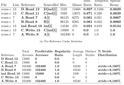
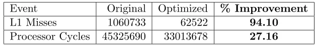
There are four distinct arrays A, B, C and D in the first use case. The functions do sum() and do mult() are called once per timestep. This program was compiled and traced under our framework on a Power4 platform using the IBM xlc compiler A cache with the following parameters was simulated: cache size=256 KB, associativity=8, line size=128, writeback cache, LRU replacement policy. This configuration is similar to the L2 cache of the Itanium2 processor [46]. The per-reference results generated by the simulator are shown in Figure 2.9. Figure 2.9(a) shows the cache metrics generated by the simulator, and Figure 2.9(b) shows the stream metrics generated by the PRSD detector.

Analysis

The reference name shown in the results has the following syntax: Variable-Name Accesstype id. VariableNameis the symbolic identifier that corresponds to the mem-ory address being accessed. Accesstypecan be eitherReadorWrite. Finally, iddenotes the unique numerical identifier for this access instruction in the executable code of the target. This syntax is used in all the use cases presented in this work.

(48)

with very low cache hit rates. The evictors for each reference are shown in Figure 2.10. The figure shows that in addition to poor locality, the D Read 12and C Read 11 references are also the top evictors for all the remaining references. Thus the references to D and C bring in data into the cache that is not reused (as indicated by their low spatial reuse values) and evict a significant amount of pre-resident data from the cache (as indicated by the per-reference evictors).

A look at the source code shows the cause of this behavior. The D Read 12 and C Read 11references are potentially sparse indirect reads on an array, indexed by the array ind[]. The remainder of the read references (A Read 7,B Read 8andind Read 10) are all direct array accesses, with regular single strided access patterns.

Miss Temporal Spatial File Line Reference SourceRef Hits Misses Ratio Ratio Reuse reuse.c 13 D Read 12 D[ind[i]] 1532 13468 0.897 0.1566 0.0639 reuse.c 13 C Read 11 C[ind[i]] 1929 13071 0.871 0.320 0.0639 reuse.c 7 A Read 7 A[i] 96125 6275 0.061 0.021 0.9867 reuse.c 7 B Read 8 B[i] 96135 6265 0.061 0.023 0.9860 reuse.c 13 ind Read 10 ind[i] 14530 470 0.031 0.019 0.9134 reuse.c 13 C Write 13 C[ind[i]] 15000 0 0.0 1.0 1.0

reuse.c 7 A Write 9 A[i] 102400 0 0.0 1.0 1.0

(a) Per-Reference Cache Statistics

Total Predictable Regularity Average Distinct % Stride Reference Accesses Accesses Ratio Length Strides Distribution

D Read 12 15000 0 0.0 0 0

-C Read 11 15000 0 0.0 0 0

-A Read 7 102400 102400 1.0 10240 1 stride=8,100%

B Read 8 102400 102400 1.0 10240 1 stride=8,100%

ind Read 10 15000 15000 1.0 1500 1 stride=4,100%

C Write 13 15000 0 0.0 0 0

-A Write 9 102400 102400 1.0 10240 1 stride=8,100%

(b) Per-Reference Stream Statistics

Trace Based Performance Characterization and Optimization

Contents

List of Figures

List of Tables

Chapter 1

Introduction

1.1

Problem Statement

1.2

Trace Generation

1.3

METRIC: Memory hierarchy analysis for single-threaded

benchmarks

1.4

ccSIM: Source-Code Correlated Cache Coherence

Char-acterization of OpenMP Benchmarks

1.5

Hybrid Hardware/Software Coherence Analysis

1.6

Hardware Profile-guided Automatic Page Placement for

ccNUMA

1.7

PFetch: Profile-guided Data Prefetching

Chapter 2

METRIC: Memory Tracing Via

Dynamic Binary Rewriting to

Identify Cache Inefficiencies

2.1

Summary

2.2

New Contributions

2.3

Introduction

2.4

The METRIC Framework

2.5

Trace Generation and Compression

A[i] = B[2*i+2] + C[5*i];

For ( I = 0; I < N; I++)

{

}

RSD_1 < 1, &A[0], N, 1>

RSD_3< 3, &C[0], N, 5>

RSD_2< 2, &B[2], N, 2>

2.6

Online Detection of PRSDs and RSDs

2.7

Evaluation of the Compression Scheme

2.8

Memory Hierarchy Simulation

2.9

Abstracting Trace Data

2.10

MHSim-generated Metrics

2.11

Stream-oriented Metrics

2.12

Diagnosis of Performance Problems

A[i] = B[2i+2] + C[5i];