Detailed analysis of POD method applied on turbulent ﬂow

(1)

Detailed analysis of POD method applied on turbulent flow

Radka KELLNEROVA1 Libor KUKACKA2 Vaclav URUBA3 Klara JURCAKOVA4 Zbynek JANOUR5

Abstract: Proper orthogonal decomposition (POD) of a very turbulent flow inside a street canyon is performed. The energy contribution of each mode is obtained. Also, physical meaning of the POD result is clarified. Particular modes of POD are assigned to the particular flow events like a sweep event, a vortex behind a roof or a vortex at the bottom of a street. Test of POD sensitivity to the acquisition time of data records is done. Test with decreasing sample frequency is also executed. Fur-ther, interpolation of POD expansion coefficient is performed in order to test possible increase in sample frequency and get new information about the flow from the POD analysis. We tested a linear and a spline type of the interpolation and the linear one carried out a slightly better result.

1 I

NTRODUCTION

Proper orthogonal decomposition (POD) appears to be a useful tool for analysing of a turbulent flow. Lumley [1] introduced POD into the turbulent flow, however this method is independently used under several names like Karhunen-Loeve decomposition, principal component analysis (PCA), empirical or-thogonal functions (EOF) or singular value decomposition (SVD).

POD is linear method applied to a non-linear problem. To understand its mathematical background, nice introduction to the PCA can be found in Shlens [2] or Smith [3]. Mathematically comprehensive studies and general overviews of application of POD are published in Aubry [4], Berkooz [5] or Tropea et al. [6]. In this project, we deal with a flow generated by a very rough surface, where intensity of turbulence reaches up to 20% at double height of the roughness. Structures in such a turbulent flow are very complex. Since only limited information can be carried out by the current measuring techniques, the de-tection of coherent structures is therefore difficult. The mathematical techniques like Quadrant analysis or Wavelet analysis are useful for detection of an interesting event at one point in the space. Neverthe-less, they are unable to provide any spatial information about the surrounded flow, so their output cannot be properly verified. On the other hand, with having the velocity information from the whole space and time, the flow events become to be somehow unclear in the internal chaos of the turbulent motion. POD can decompose a very complex flow into more simple modes in every spatial point, regardless the complexity of the system.

Two versions of POD exist, classic and snapshotone (Sirovich [7]). The latter one is less compu-tationally demanding. Snapshot version of POD is based on the cross-correlation between individual snapshots of velocity fluctuations. The goal is to find a new orthogonal basis (i.e. modes) with a max-imum average projection of the fluctuations on the basis. The new basis can be re-ordered after its contribution to the TKE in the flow. It means, the first mode (i.e. eigenvector) would contain the highest portion of TKE, the second mode (i.e. eigenvector) would contain a little bit lower TKE, and so on. The method POD is orthogonal what is convenient from mathematical point of view. The original field of the fluctuation can be linearly superposed from particular modes. When involving only the most dominant modes into the superposition, the complexity of the system is reduced.

1 Radka Kellnerova, Institute of Thermomechanics,

Department of Meteorology and Environment Protection, Charles University, [email protected] 2 Libor Kukacka, Institute of Thermomechanics,

Department of Meteorology and Environment Protection, Charles University, [email protected] 3 Vaclav Uruba, Institute of Thermomechanics, [email protected]

4 Klara Jurcakova, Institute of Thermomechanics, [email protected] 5 Zbynek Janour, Institute of Thermomechanics, [email protected]

(2)

2 E

XPERIMENTAL SET

-

UP

The surface boundary layer is generated in a wind-channel using a very rough terrain. The channel has the dimension of 0.25 m x 0.25 m in cross-section and 3 m in longitudinal direction (Figure 1). Reference wind speed in the axis of the channel is 5 m/s. Reynolds building number is

Re2H= U2H_ν.2H = 40000,

derived from velocityU₂Hat the double level of the building heightH and kinematic viscosityν.

20

50 mm

50

mm

50 mm

30 _{50 mm}

50 mm

250 mm

Z

X

Measuring area Y

50

//

50

2 000 mm

3000 mm

//

Laser

Figure 1: Left: Scheme of buildings with flat roof (upper) and pitched roof (lower). Right: Scheme of model of street canyons inside the channel. Flow is coming from the left side. Green area denotes the light sheet of the laser.

The roughness elements are built from long series of identical and parallel street canyons (see Figure 1 -right). The area of interest lies as far downstream as possible from the channel entrance in order to pro-vide a sufficient fetch for development of a well-balanced turbulent boundary layer (Cheng & Castro [8]). Two geometries of roof are used - triangle and flat shape. Scale in which the model is manufactured is 1:400, so the 20 m high real building are represented by the modeled canyon with 50 mm in dimension. The ratio of the cross-section of the model with respect to the cross-section of the channel is 20%. This brings an undesirable aerodynamic blocking of the approaching flow due to the presence of internal boundary layer. Therefore, the results of measurement can be hardly applicable on the real conditions. Nevertheless, a wind-tunnel experiment with the identical model was performed before this campaign. We can conclude that dynamics of the urban canopy layer (UCL) and lower part of roughness layer (RL) - what is approximately up to Z/H=1.5 - match well with a properly modeled boundary layer in the wind-tunnel. Above this level, the higher is the elevation, the bigger deviation from correct boundary layer occurs.

Time-resolved Particle Image Velocimetry (TR-PIV) with high repetition rate (500 Hz) is used to reveal 2-D instantaneous vectors in vertical plane. Flow is filled by tracer particles of oily substance with mean radius of 1μm. Due to high intensity of turbulence, the oil droplets are evenly distributed in the chamber what produces images of a good reliability. One run of PIV measurement consists from 1635 snapshots, each of them with 4800 velocity vectors. The spatial resolution turns out to be 1.2 mm x 1.2 mm. The acquisition time is reduced on 3.2 s due to camera memory storage limit. In table 2 below, the parameters of PIV set-up are published.

Commercial software for PIV (DynamicStudio v. 3.00.) allows us to post-process data and reject spu-rious vectors. Series of validations and filters are applied on dataset in order to identify the spuspu-rious vectors and replace them with better estimations.

Corrected PIV vector fields serve as a data input for calculation of POD. We used a snapshot version of POD method designed after Hertwig [9] algorithm. The calculation involves two velocity components, longitudinal (U) and vertical (W) one. For plotting of a particular mode, TECPLOT picture with pseudo-streamlines is used to display the dominant dynamical modes.

3 R

ESULTS OF

POD

3.1 CONVERGENCE OFPODMODES

(3)

Table 2 Diode pumped Nd:YLF laser

Repetition rate 500 - 1000 Hz

Resolution 1280 x 1024 pxs

Interrogation area 32 x 32 pxs

Overlapping 50% (80 x 64 vectors)

Energy 10 mJ

Area 100 x 100 mm

Acquisition time 3.2 s

a highly coherent structure. Some of flow exhibits very high relative contribution in the most dominant mode (e.g. 40%).

The Figure 2 shows the relative contribution of each mode for both roof arrangements. The relative value of TKE is depicted on the left side. The very first mode of the flow above the pitched roofs (red triangles) contains around 32% of energy what is rather a high number. The other contributions fall down very quickly. The following modes have only 7% and 6% of TKE and the rest of values diminish very soon. The flow above flat roof (grey squares) is a slightly less coherent in comparison to the pitched case, the contribution from the most dominant mode is only 27%. Second mode contains again 7% of TKE and the next one 4%.

On the right side of the picture is a cumulative contribution for both arrangements. The faster is the rate of the convergence, the higher level of coherency should be in the system. The pitched case converges slightly faster than the flat case. We can conclude that pitched roofs generate a flow with higher variation of velocity (e.g. larger fluctuations from the mean value) in an organised sense (e.g. within an organised motion).

100 101 102 103 0

5 10 15 20 25 30 35

Mode number

Relative contribution [%]

Convergence of eigenvalues − Pitched and flat roof

100 101 102 103 0

10 20 30 40 50 60 70 80 90 100

Mode number

Cumulative relative contribution [%]

Convergence of eigenvalues − Pitched and flat roof

Pitched roof Flat roof Pitched roof

Flat roof

(4)

3.2 PODMODES

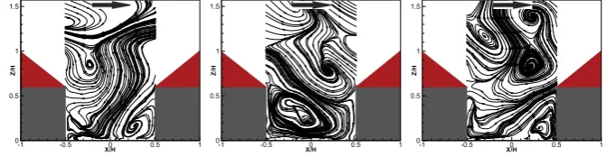
Modes are function of space. The fourth most dominant modes from the pitched case are displayed in Figure 3. The pictures of mode represent the following dynamical phenomena with percentage of TKE in parentheses:

Mode 1: vortex behind the roof (32%) Mode 2: recirculation between the wall (7%) Mode 3: sweep/ejection (6%)

Mode 4: vortex near the bottom of street (4%)

X/H

Z/

H

-1 -0.5 0 0.5 1 0

0.5 1 1.5

X/H

Z/

H

-1 -0.5 0 0.5 1

0 0.5 1 1.5

X/H

Z/

H

-1 -0.5 0 0.5 1 0

0.5 1 1.5

X/H

Z/

H

-1 -0.5 0 0.5 1

0 0.5 1 1.5

Figure 3: From the left: the first, the second, the third and the fourth POD mode of flow above the pitched roofs.

The reconstruction of the original (instantaneous) vector field can be expressed by the expansion

u(−→x , t) =u+ Σiai(t)θi(−→x)

whereai(t) is the expansion coefficient for corresponding mode θi(−→x). Coefficient acts as a weight

factor for each mode. In particular time it can reach a large value. In this particular moment, the mode plays an important role in the flow.

Others modes contribute by 2.5% or less to TKE, so the importance of the further modes is much lower. Comparison of maximum of the expansion coefficients for modes No. 5, 6 and 7 shows that their absolute peaks reaches one third of the peak of the first mode. Also, the standard deviation of their expansion coefficients is of 30% of standard deviation of the first mode (see for illustration Figure 9). From statistic point of view, these modes are much less relevant. Still, from time to time, they can be significantly strong in the flow field and affect a momentum flux.

The fifth mode might represent the impact of the approaching flow on the downstream roof (see Fig-ure 4), the sixth is likely a simple flush of wind into the canyon along the downstream part of the upstream roof. The seventh mode could be again the backward flow inside the street canyon as a consequence of a hit of approach wind on the roof under a slightly different angle. However, with increasing number of mode the physical interpretation is more and more difficult to be revealed and even before-mentioned interpretations can be misleading.

X/H

Z/

H

-1 -0.5 0 0.5 1

0 0.5 1 1.5

X/H

Z/

H

-1 -0.5 0 0.5 1

0 0.5 1 1.5

X/H

Z/

H

-1 -0.5 0 0.5 1

0 0.5 1 1.5

Figure 4:From left: the fifth, the sixth and the seventh POD mode of flow above the pitched roofs.

(5)

coefficients and standard deviations are around half value as well. So the particular modes do not exhibit such dominance over the field. We can conclude that flow above flat roofs is dynamically ’calmer and smoother’. Consistently, based on the PIV records, the flow above flat roofs is essentially less disturbed than in the pitched case.

X/H

Z/

H

-1 -0.5 0 0.5 0

0.5 1 1.5

X/H

Z/

H

-1 -0.5 0 0.5 0

0.5 1 1.5

X/H

Z/

H

-1 -0.5 0 0.5 0

0.5 1 1.5

X/H

Z/

H

-1 -0.5 0 0.5 0

0.5 1 1.5

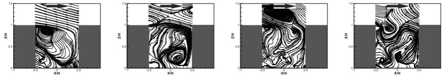
Figure 5:From left: the first, the second, the third and the fourth POD mode of flow above the flat roofs.

3.3 SENSITIVITY

We tested sensitivity of POD method on the sample frequency and the acquisition time.

SENSITIVITY TO A SAMPLE FREQUENCY

The turbulent flow above thepitchedroofs is used as data input. The primary measurement is done with sample frequency of 500 Hz. When we remove every 2nd snapshot from primary (full) dataset, we get a reduced dataset with sample frequency of 250 Hz. Since we can remove every first snapshot (odd snapshots) or every second snapshot (even snapshots), we performed the test for both types of reductions.

The temporal evolution of the expansion coefficients for the reduced datasets is displayed in Figure 6. The first expansion coefficient (corresponding to Mode 1) from the full dataset is labeledMode 1 v.1.The first expansion coefficients for Mode 1 from POD applications on reduced datasets are labeledMode 1 v.2.1(even values involved in calculation) orMode 1 v.2.2 (odd values involved in calculation).

Since half of data are missing in the reduced version, these absent data are interpolated by a linear interpolation. Left picture shows the deviation of these reduced coefficients from the primary ones. The deviation is actually very small, only minute discrepancies are visible between the primary measurement and the reduced versions.

Further reducing in the frequency is performed. When we involve into the calculation every4th,8thand 16th _{snapshot, we get very sparse data-sets with a poor temporal resolution. These data-ranks will be}

called4th,8th or 16th set. In the right picture of Figure 6 we can see the discrepancies between the expansion coefficients growing proportionally to the reducing in the sample frequency. When we look at 16th_{set, the majority of the information is already lost.}

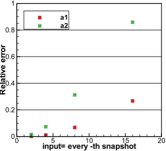
The deviation of the interpolated curves (for mode 1 and 2) from the primary curves are depicted in Figure 7. The deviation raises up very quickly with an increase in the reduction. The higher mode exhibit a dramatic deviation indeed.

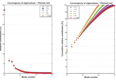
Figure 8 - left displays the relative contributions to the total TKE for the various reductions and the full dataset. The number of modes is different for each dataset, thus the count of mode differs as well. The plot therefore shows only the first hundred of modes. The important information is the percentage value on the ordinate. The TKE contribution from the first mode from almost all the reductions exhibit the same values, except the16th set. Moreover, the two highest reductions exhibit a higher scatter.

In Figure 8 - right, the cumulative relative contribution for all reductions is depicted. The rate of conver-gence is very distinguish for a highly reduced data, since the two highest reductions exhibit a different slope. Such a steep slope is given by the lower number of involved modes in the reduced dataset (e.g. the16th set contains only 102 modes). The rate therefore more quickly reaches the 100%. It has to be emphasised that the similar picture would be obtained from the classic POD approach. Detailed inspection also verified that for this16th set the spatial shape of modes differs from the primary POD analysis.

(6)

ener-Snapshot

E

x

pa

ns

io

n

c

oe

ff

ic

ie

n

t

0 50 100 150 200 250 300

-80 -40 0 40 80

mode1 v.1 mode2 v.1 mode1 v.2.1 mode2 v.2.1 mode1 v.2.2 mode2 v.2.2

Snapshot

E

x

pa

ns

ion

c

oe

ff

ic

ie

nt

0 50 100 150 200 250 300

-80 -40 0 40 80

mode1 v.1 mode1 v.4 mode1 v.8 mode1 v.16

Figure 6: Left: Time-evolution of the coefficients from the primary measurement (v.1 - thick lines) and the reduced version (v.2.1 and v.2.2 - tiny lines). Right: The comparison of time-evolution among the coefficients from reduced4th,8thand16thdataset.

input= every -th snapshot

Re

la

ti

v

e

rr

o

r

0 5 10 15 20

0 0.2 0.4 0.6 0.8 1

a1 a2

Figure 7:Relative error of reduced POD coefficientsa₁anda₂with respect to the primary POD data.

getic scheme of relative contribution follows almost the primary version and spatial patterns of POD modes keep the same shape as primary ones. However with a lower frequency, the coefficients start to deviate markedly. Notwithstanding, the shapes of modes are still similar. Only the rate of the energy convergence is very sensitive on number of snapshots involved in the calculation.

We can also conclude that 16th set contains too little information about dynamics and POD analysis yields up a completely different results.

SENSITIVITY TO AN ACQUISITION TIME

Since the acquisition time of 3.2 s for each PIV measurement run is very short, we repeated measure-ment for two times. The sample frequency was kept on 500 Hz what gives the acquisition time of 3.2 s. Third measurement was done with sample frequency of 100 Hz and acquisition time of 16.3 s. By this, we get total acquisition time of 22.7 s.

(7)

100 101 102 103 0

5 10 15 20 25 30 35

Mode number

Convergence of eigenvalues − Pitched roof

100 101 102 103

0 10 20 30 40 50 60 70 80 90 100

Mode number

v.2.1 v.2.2 v.4 v.8 v.16 v.1 (full) v.2.1

v.2.2 v.4 v.8 v.16 v.1 (full)

Figure 8: Changes in relative contribution to the TKE (ordinate) for different modes (abscissa) and reduced data input (color).

to each other with 2.2% of difference for mean W-component. The standard deviation has scatter about 11% resp. 6% for U- resp. W-component. Also difference among TKE, calculated from two components herein, is only 3%.

The POD results from all three runs were analysed and mutually compared. For each run the expan-sion coefficients were carried out. The overview of their standard deviation and their maximum values in absolute sense from all three pitched-case runs (labelled as Prun1, Prun 2 and Prun 3) is depicted in Figure 9. Figure shows the values for the first 50 expansion coefficients, since the both statistics monotonously decrease and higher modes thus have only a minute importance. All three runs exhibit the similar behavior. Standard deviations σ (squares) collapsed into one curve. The maximum val-ues (circles) slightly differ from each other in low mode number. However this is natural, since some strong events happen rather from time to time. The number 1635 of snapshots does not have to cover outstanding dynamical situation every time.

Finally, we performed POD analysis on ensemble of all data we had for the pitched shape of roof. The velocity fluctuations from all three runs were collected together into one dataset. According to Tropea et al. [6], the observations (snapshots) have to be linearly independent. Among others, it means that the number of snapshots has to be lower than the number of positions used for calculation. However, the number of positions can be simply increased by a higher overlapping in post-processing of PIV raw images. The number of positions in our case reaches 10, 000 values, whereas the total count of snapshots is 4905.

POD was applied to this collected ensemble and again, the results were compared with individual re-alisations. Difference between individual runs from the ensemble using Frobenius norm is calculated for a few first modes. Values are presented in the table 1. The relative deviations from the ensemble are rather small. The more important mode, the smaller deviation occurs. This can be consider as a proof either for verification if the acquisition time of PIV records is at least of reasonable length or for robustness of POD methods since it brings similar results for different time-pieces of flow.

(8)

0 5 10 15 20 25 30 35 40 45 50 0

20 40 60 80 100 120

Mode number

Maximum value and

σ

Maximum value and σ for each run

σ Prun1

Max Prun1

σ Prun2

Max Prun2

σ Prun3

Max Prun3

Figure 9: Changes in relative contribution to the TKE (ordinate) for different modes (abscissa) and reduced data input (colour).

Table 1 Run 1 Run 2 Run 3

Mode 1 4.2 3.6 2.3

Mode 2 10.6 13.1 9.9

Mode 3 17.0 10.6 10.8

Mode 4 23.6 16.5 14.5

Table 1:Relative deviation of particular runs from ensemble [%].

that three runs have a little bit different values of relative contribution the TKE from the first modes. In the right part of the Figure 10 the rates of convergence collapse for all the runs, regardless the length of the acquisition time. Furthermore, the ensemble and the third run exhibit the highest similarity, what suggests that the third run is the best representation of the flow dynamics in the street canyon.

3.4 INTERPOLATION OFPOD

Interpolation of POD is procedure based on a simple assumption: coherent structures can be considered as temporally continuous as pointed out Bouhoubeiy & Drualult [10]. Ordinary velocity data cannot be freely interpolated, since the dynamics of the structures would not be captured inside a new data. However, regarding the temporal evolution of structure as a smooth process, the time-interpolation of POD expansion coefficients can represent the missing dynamics reliably. Bouhoubeiy & Drualult [10] in their paper verified that POD interpolation is correct from mathematical point of view. Notwithstanding, its physical meaning has to be tested.

For the verification purpose, we use before-mentioned half-dataset reduced from the primary POD mea-surement (with every second snapshots taken into the account). Its expansion coefficients have two-times lower temporal resolution and the number of modes is two-time lower (i.e. 817).

Then, by a linear and a spline interpolations, we added the missing data into the temporal series of the expansion coefficients. Next step was to perform a reconstruction using all (including of the interpolated ones) expansion coefficients. The reconstruction follows the formula below, whereK is the number of modes at disposal.

u(−→x , t) =u+ ΣK

i=1ai(t)θi(−→x)

(9)

100 101 102 103 0

5 10 15 20 25 30 35

Mode number

run1 run2 run3 All 3 runs

100 101 102 103

0 10 20 30 40 50 60 70 80 90 100

Mode number

run1 run2 run3 All 3 runs

Figure 10: Changes in relative contribution to the TKE (ordinate) for different modes (abscissa) and reduced data input (color).

level of a dynamical complexity, therefore the reconstruction of each snapshot reaches different level of the accuracy. Former attempt with reconstruction of the flow field by the POD method showed that snapshot No. 204 is moderately complex in terms of dynamics and it provides a good representation of flow at the instant of time.

Comparison of the original snapshot No. 204 (frequency 500 Hz) and the interpolated reconstruction (frequency re-doubled from 250 Hz to 500 Hz) was done using Frobenius norm. The final results for the interpolated snapshot are depicted in Figure 11. In the upper part of the picture, the original snapshot from the full dataset is displayed. Lower part of the picture shows reconstruction of the snapshot No. 204 by the linear interpolation (on the left) and by the spline interpolation (on the right).

The deviation between the linear interpolation and the original snapshot is 11%. Deviation between the spline interpolation and the original snapshot is 12%. Thus, the method of interpolation does not influence the accuracy of the reconstruction. The deviation of 11% is not high. Since the Frobenius norm is rather strict, deviation of 11% suggests that method of the interpolation based on POD can bring a reliable data. However, the method deserves a further investigation before any final conclusion of its reliability will be draft.

4 C

ONCLUSION

The detailed inspection of POD analysis was done. Velocity data from the wind-channel campaign serve as an input for the POD analysis. The modes and the expansion coefficients were investigated carefully. The time when the peaks of the coefficients appear in the time-evolution is linked to the PIV record. By this, we can verify that POD modes can really express physical phenomena.

(10)

X [pxs]

Y [pxs]

Snapshot 204 − Magnitude of velocity [m/s]

5 10 15 20 25 30 35 40

10 20 30 40 50 60

0.5 1 1.5 2 2.5 3 3.5 4 4.5 5 5.5 6

X [pxs]

Z [pxs]

POD synthesis of interpolated data (linear) − 817 Modes, 1634 snapshots Magnitude of velocity [m/s]

5 10 15 20 25 30 35 40

10 20 30 40 50 60

0 1 2 3 4 5 6

X [pxs]

Z [pxs]

POD synthesis of interpolated data (spline) − 817 Modes, 1634 snapshots Magnitude of velocity [m/s]

5 10 15 20 25 30 35 40

10 20 30 40 50 60

0 1 2 3 4 5 6

Figure 11:Upper: Original snapshot No. 204. Magnitude of velocity is plotted in colour. Lower: Recon-struction based on the temporal interpolation of expansion coefficients. On the left: linear interpolation. On the right: Spline interpolation.

The backward interpolation based on POD was tested. Synthesis showed up that interpolated data differ from the original one by 11-12%. However, the legitimacy of the interpretation of the POD interpolation should be further verified.

Acknowledgement Authors kindly thank for support from AV0Z20760514 and the Project M100760901 of Academy of Science of the Czech Republic.

R

EFERENCES

[1] J L Lumley, The structure of inhomogeneous turbulent flows. In A. M. Yaglom and V. I. Tatarski, editors, Atmospheric Turbulence and Radio Wave Propagation, 1967, 166-178.

[2] J Shlens,A Tutorial on Principal Component Analysis. ’La Jolla, CA 92037: Salk Institute for Biolog-ical Studies’, 2005. URL - http://www.snl.salk.edu/ shlens/

[3] L I Smith,A tutorial on Principal Components Analysis, 2002. URL - http://www.cs.otago.ac.nz/

[4] N Aubry, R Guyonnet, R Lima,Spatiotemporal Analysis of Complex Signals: Theory and Applica-tions, Journal of Statistical Physics,64, 1991, 683-739.

(11)

[6] C Tropea, A Yarin, J Foss, Springer Handbook of experimental Fluid Mechanics, Springer, 2007, 1346-1370.

[7] L Sirovich, Turbulence and the dynamics of coherent structures. Part I: Coherent structures, Quaterly of Applied Mathematics,45, 1987, 561-571.

[8] H Cheng, I P Castro, Near-Wall Development After a Step Change in Surface Roughness. Boundary- Layer Meteorology,105, 2002, 411-432.

[9] D Hertwig, Detection of coherent structures in atmospheric boundary layer flows: a comparative wind tunnel study using POD, LSE and wavelets, Diploma thesis, University of Hamburg, 2009.