Hard Isogeny Problems over RSA Moduli and Groups with Infeasible Inversion

(1)

Hard Isogeny Problems over RSA Moduli and

Groups with Infeasible Inversion

Salim Ali Altu˘g∗ Yilei Chen†

May 14, 2019

Abstract

We initiate the study of computational problems on elliptic curve isogeny graphs defined over RSA moduli. We conjecture that several variants of the neighbor-search problem over these graphs are hard, and provide a comprehensive list of cryptanalytic attempts on these problems. Moreover, based on the hardness of these problems, we provide a construction of groups with infeasible inversion, where the underlying groups are the ideal class groups of imaginary quadratic orders.

Recall that in a group with infeasible inversion, computing the inverse of a group element is required to be hard, while performing the group operation is easy. Motivated by the potential cryptographic application of building a directed transitive signature scheme, the search for a group with infeasible inversion was initiated in the theses of Hohenberger and Molnar (2003). Later it was also shown to provide a broadcast encryption scheme by Irrer et al. (2004). However, to date the only case of a group with infeasible inversion is implied by the much stronger primitive of self-bilinear map constructed by Yamakawa et al. (2014) based on the hardness of factoring and indistinguishability obfuscation (iO). Our construction gives a candidate without using iO.

∗

Boston University. [email protected]. Research supported by the grant DMS-1702176.

†

(2)

1 Introduction

Let G denote a finite group written multiplicatively. The discrete-log problem asks to find the

exponentagivengandga∈_G. In the groups traditionally used in discrete-log-based cryptosystems, such as (Z/qZ)∗ [DH76], groups of points on elliptic curves [Mil85,Kob87], and class groups [BW88, McC88], computing the inversex−1 =g−a given x=ga is easy. We sayGis a group with infeasible

inversion if computing inverses of elements is hard, while performing the group operation is easy (i.e. giveng,ga,gb, computing ga+b is easy).

The search for a group with infeasible inversion was initiated in the theses of Hohenberger [Hoh03] and Molnar [Mol03], motivated with the potential cryptographic application of constructing a directed transitive signature. It was also shown by Irrer et al. [ILOP04] to provide a broadcast encryption scheme. The only existing candidate of such a group, however, is implied by the much stronger primitive of self-bilinear maps constructed by Yamakawa et al. [YYHK14], assuming the hardness of integer factorization and indistinguishability obfuscation (iO) [BGI+01,GGH+13].

In this paper we propose a candidate trapdoor group with infeasible inversion without using iO. The underlying group is isomorphic to the ideal class group of an imaginary quadratic order (henceforth abbreviated as “the class group”). In the standard representation1 of the class group, computing the inverse of a group element is straightforward. The representation we propose uses the volcano-like structure of the isogeny graphs of ordinary elliptic curves. In fact, the initiation of this work was driven by the desire to explore the computational problems on the isogeny graphs defined over RSA moduli.

1.1 Elliptic curve isogenies in cryptography

An isogenyϕ:E1→E2 is a morphism of elliptic curves that preserves the identity. Given two isoge-nous elliptic curvesE1,E2 over a finite field, finding an explicit rational polynomial that represents an isogeny fromE1 toE2 is traditionally called thecomputational isogeny problem.

The study of computing explicit isogenies began with the rather technical motivation of improving Schoof’s polynomial time algorithm [Sch85] to compute the number of points on an elliptic curve over a finite field (the improved algorithm is usually called Schoof-Elkies-Atkin algorithm, cf. [CM94,

Sch95,E+98] and references therein). A more straightforward use for explicit isogenies is to transfer the elliptic curve discrete-log problem from one curve to the other [Gal99, GHS02, JMV05]. If for any two isogenous elliptic curves computing an isogeny from one to the other is efficient, then it means the discrete-log problem is equally hard among all the curves in the same isogeny class.

The best way of understanding the nature of the isogeny problem is to look at the isogeny graphs. Fix a finite field k and a prime ` different than the characteristic of k. Then the isogeny graph

G`(k) is defined as follows: each vertex in G`(k) is a j-invariant of an isomorphism class of curves;

two vertices are connected by an edge if there is an isogeny of degree`over kthat maps one curve to another. The structure of the isogeny graph is described in the PhD thesis of Kohel [Koh96]. Roughly speaking, a connected component of an isogeny graph containing ordinary elliptic curves looks like avolcano (termed in [FM02]). The connected component containing supersingular elliptic curves, on the other hand, has a different structure. In this article we will focus on the ordinary case.

1

(4)

End(E)

O_K

Z[π]

`-isogenies

m-isogenies

Figure 1: Examples of isogeny graphs. Left: a connected component ofG`(k), and the corresponding

tower of imaginary quadratic orders [Feo17]; Right: the vertex set is EllO(C) for an imaginary

quadratic orderO, the edges represent (isomorphic classes of) isogenies of degrees `,m.

A closer look at the algorithms of computing isogenies. Letkbe a finite field ofqelements,

`be an integer such that gcd(`, q) = 1. Given thej-invariant of an elliptic curveE, there are at least two different ways to find all thej-invariants of the curves that are`-isogenous to E (or to a twist ofE) and to find the corresponding rational polynomials that represent the isogenies:

1. Computing kernel subgroups ofEof size`, and then applying V´elu’s formulae to obtain explicit isogenies and thej-invariants of the image curves,

2. Calculating thej-invariants of the image curves by solving the`thmodular polynomial Φ` over

k, and then constructing explicit isogenies from these j-invariants.

Both methods are able to find all the`-isogenous neighbors over kin time poly(`,log(q)). In other words,over a finite field, one can take a stroll around the polynomial-degree isogenous neighbors of a given elliptic curve efficiently.

However, for two random isogenous curves over a sufficiently large field, finding an explicit isogeny between them seems to be hard, even for quantum computers. The conjectured hardness of com-puting isogenies was used in a key-exchange and a public-key cryptosystem by Couveignes [Cou06] and independently by Rostovtsev and Stolbunov [RS06]. Moreover, a hash function and a key ex-change scheme were proposed based on the hardness of computing isogenies over supersingular curves [CLG09, JF11]. Isogeny-based cryptography is attracting attention partially due to its conjectured post-quantum security.

1.2 Isogeny graphs over RSA moduli

Let p, q be primes and let N = pq. In this work we consider computational problems related to elliptic curve isogeny graphs defined over Z/NZ, where the prime factors p, q of N are unknown.

An isogeny graph over Z/NZ is defined first by fixing the isogeny graphs over Fp and Fq, then

taking a graph tensor product; obtaining the j-invariants in the vertices of the graph over Z/NZ

by the Chinese remainder theorem. Working over the ring Z/NZ without the factors of N creates

(5)

Z/NZ

j0

j1 j2

j3

` m m `

Z/NZ

j−1 = ?

... j0

j1

j0,1 = ?

j0,2 = ?

...

`

` `

`

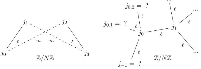
Figure 2: Left: the (`, m)-isogenous neighbor problem where gcd(`, m) = 1. Right: the (`, `2 )-isogenous neighbor problem.

Basic neighbor search problem overZ/NZ. When the factorization ofN is unknown, it is not

clear how to solve the basic problem of finding (even one of) the `-isogenous neighbors of a given elliptic curve. The two algorithms over finite fields we mentioned seem to fail overZ/NZsince both

of them require solving polynomials over Z/NZ, which is hard in general when the factorization of

N is unknown. In fact, we show that if it is feasible to find all the `-isogenous neighbors of a given elliptic curve overZ/NZ, then it is feasible to factorize N.

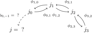
Joint-neighbor search problem over Z/NZ. Suppose we are given several j-invariants over Z/NZ that are connected by polynomial-degree isogenies, we ask whether it is feasible to compute

their joint isogenous neighbors. For example, in the isogeny graph on the LHS of Figure2, suppose we are given j0, j1, j2, and the degrees ` between j0 and j1, and m between j0 and j2 such that gcd(`, m) = 1. Then we can find j3 which is m-isogenous toj1 and `-isogenous toj2, by computing the polynomial f(x) = gcd(Φm(j1, x),Φ`(j2, x)) over Z/NZ. When gcd(`, m) = 1 the polynomial

f(x) turns out to be linear with its only root beingj3, hence computing the (`, m) neighbor in this case is feasible.

However, not all the joint-isogenous neighbors are easy to find. As an example, consider the following (`, `2)-joint neighbor problem illustrated on the RHS of Figure2. Suppose we are givenj0andj1that are`-isogenous, and asked to find anotherj-invariantj−1which is`-isogenous toj0and `2-isogenous toj1. The natural way is to take the gcd of Φ`(j0, x) and Φ`2(j₁, x), but in this case the resulting polynomial is of degree` > 1 and we are left with the problem of finding a root of it over Z/NZ,

which is believed to be computationally hard without knowing the factors of N.

Currently we do not know if solving this problem is as hard as factoring N. Neither do we know of an efficient algorithm of solving the (`, `2)-joint neighbor problem. We will list our attempts in solving the (`, `2)-joint neighbor problem in Section 5.2.

The conjectured computational hardness of the (`, `2)-joint neighbor problem is fundamental to the infeasibility of inversion in the group we construct.

1.3 Constructing a trapdoor group with infeasible inversion

(6)

F83

j0 = 15

j1 = 48

j2 = 23

j3 = 29

j4 = 34

j5 = 55

j6 = 71

F83

j0 = 15

j1 = 48

j2 = 23

j3 = 29

j4 = 34

j5 = 55

j6 = 71

F83

j0 = 15

j1 = 48

j2 = 23

j3 = 29

j4 = 34

j5 = 55

j6 = 71

F83

j0 = 15

j1 = 48

j2 = 23

j3 = 29

j4 = 34

j5 = 55

j6 = 71

F83

j0 = 15

j1 = 48

j2 = 23

j3 = 29

j4 = 34

j5 = 55

j6 = 71

F83

j0 = 15

j1 = 48

j2 = 23

j3 = 29

j4 = 34

j5 = 55

j6 = 71

F83

j0 = 15

j1 = 48

j2 = 23

j3 = 29

j4 = 34

j5 = 55

j6 = 71

F173

j0= 2

j1 = 162

j2 = 36

j3 = 117

j4 = 134

j5 = 116

j6= 167

F173

j0= 2

j1 = 162

j2 = 36

j3 = 117

j4 = 134

j5 = 116

j6= 167

F173

j0= 2

j1 = 162

j2 = 36

j3 = 117

j4 = 134

j5 = 116

j6= 167

F173

j0= 2

j1 = 162

j2 = 36

j3 = 117

j4 = 134

j5 = 116

j6= 167

F173

j0= 2

j1 = 162

j2 = 36

j3 = 117

j4 = 134

j5 = 116

j6= 167

F173

j0= 2

j1 = 162

j2 = 36

j3 = 117

j4 = 134

j5 = 116

j6= 167

F173

j0= 2

j1 = 162

j2 = 36

j3 = 117

j4 = 134

j5 = 116

j6= 167

−−−→

CRT

Z14359

j0 = 12631

j1 = 7601

j2 = 1766

j3 = 4096

j4 = 7919

j5 = 2711

j6 = 1897

Z14359

j0 = 12631

j1 = 7601

j2 = 1766

j3 = 4096

j4 = 7919

j5 = 2711

j6 = 1897

Z14359

j0 = 12631

j1 = 7601

j2 = 1766

j3 = 4096

j4 = 7919

j5 = 2711

j6 = 1897

Z14359

j0 = 12631

j1 = 7601

j2 = 1766

j3 = 4096

j4 = 7919

j5 = 2711

j6 = 1897

Z14359

j0 = 12631

j1 = 7601

j2 = 1766

j3 = 4096

j4 = 7919

j5 = 2711

j6 = 1897

Z14359

j0 = 12631

j1 = 7601

j2 = 1766

j3 = 4096

j4 = 7919

j5 = 2711

j6 = 1897

Z14359

j0 = 12631

j1 = 7601

j2 = 1766

j3 = 4096

j4 = 7919

j5 = 2711

j6 = 1897

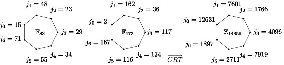
Figure 3: A representation ofCL(−251) by a 3-isogeny volcano over_Z14359 of sizeh(−251) = 7. The

F83 part is taken from [RS06].

imaginary quadratic orderO. The group of invertibleO-ideals acts on the set of elliptic curves with endomorphism ringO. The ideal class groupCL(O) acts faithfully and transitively on the set

EllO(k) ={j(E) :E with End(E)' O}.

In other words, there is a map

CL(O)×EllO(k)→EllO(k), (a, j)7→a∗j

such thata∗(b∗j) = (ab)∗j for alla,b∈ CL(O) andj∈EllO(k); for any j, j0 ∈EllO(k), there is a uniquea∈ CL(O) such thatj0=a∗j. The cardinality of EllO(k) equals to the class numberh(O).

We are now ready to provide an overview of the TGII construction with a toy example in Figure3.

Parameter generation. To simplify this overview let us assume that the group CL(O) is cyclic, in which case the group Gwith infeasible inversion is exactly CL(O) (in the detailed construction we

usually choose a cyclic subgroup ofCL(O)). To generate the public parameter for the group CL(O), we choose two primesp, q and curves E0,Fp overFp and E0,Fq overFq such that the endomorphism

rings ofE0,Fp and E0,Fq are both isomorphic to O. Let N =p·q. Let E0 be an elliptic curve over Z/NZ as the CRT composition ofE0,Fp and E0,Fq. The j-invariant ofE0, denoted asj0, equals to

theCRT composition of thej-invariants of E0,Fp and E0,Fq. The identity ofCL(O) is represented by

j0. The public parameter of the group is (N, j0).

In the example of Figure3, we set the discriminantDof the imaginary quadratic orderOto be−251. The group order is then the class numberh(O) = 7. Choose p= 83, q = 173,N =pq= 14359. Fix a curveE0 so that j(E0,Fp) = 15, j(E0,Fq) = 2, then j0 = CRT(83,173; 15,2) = 12631. The public

parameter is (14359,12631).

The encodings. We provide two types of encodings for each group element: the canonical and composable embeddings. The canonical encoding of an element is uniquely determined once the public parameter is fixed and it can be directly used in the equivalence test. It, however, does not support efficient group operations. Thecomposable encoding of an element, on the other hand, supports efficient group operations with the other composable encodings. Moreover, a composable encoding can be converted to a canonical encoding by an efficient, public extraction algorithm.

An elementx∈ CL(O) is canonically represented by thej-invariant of the elliptic curvex∗E0 (once again, obtained overFpandFq then composed byCRT), and we callj(x∗E0) the canonical encoding ofx. Note that the canonical encodings of all the elements are fixed oncej0 and N are fixed.

To make things concrete, let a = √−251 and consider the toy example above. The ideal class

(7)

canonical encoding ofxis thenj1 =CRT(83,173; 48,162) = 7601. Similarly, the canonical encodings of the ideal classes [(7,a−1₂ )], [(5,a+7₂ )], [(5,a+3₂ )], [(7,a+1₂ )], [(3,a−1₂ )] are 1766,4096,7919,2711,1897.

The composable encodings and the composition law. To generate a composable encoding of

x∈ CL(O), we factorize x asx=Q

xi∈Sx

ei

i , where S denotes a generating set, and both the norms N(xi) and the exponents ei being polynomial in size. The composable encoding ofxthen consists of

the normsN(xi) and thej-invariants ofxk_i∗E0, fork∈[ei], fori∈[|S|]. Thedegreeof a composable encoding is defined to be the product of the norms of the idealsQ

xi∈SN(xi)

ei_{. Note that the degree}

depends on the choice ofS and the factorization of x, which is not unique.

As an example let us consider the simplest situation, where the composable encodings are just the canonical encodings themselves together with the norms of the ideals (i.e. the degrees of the isogenies). Set the composable encoding of x= [(3,a+1₂ )] be (3,7601), the composable encoding of

y= [(7,a−1₂ )] be (7,1766).

Let us remark an intricacy of the construction of composable encodings. When the degrees of the composable encodings ofxandyare coprime and polynomially large, the composition ofxandycan be done simply by concatenating the corresponding encodings. To extract the canonical encoding of

x◦y, we take the gcd of the modular polynomials. In the example above, the canonical encoding of

x◦y can be obtained by taking the gcd of Φ7(7601, x) and Φ3(1766, x) overZ/NZ. Since the degrees

are coprime, the resulting polynomial is linear, with the only root being 4096, which is the canonical encoding of [(5,a+7₂ )].

Note, however, that if the degrees share prime factors, then the gcd algorithm does not yield a linear polynomial, so the the above algorithm for composition does not go through. To give a concrete example to what this means let us go back to our example: if we represent y = [(7,a−1₂ )] by first factorizingy as [(3,a+1₂ )]2 _{we then get the composable encoding of}_y _{as (3}_,₍₇₆₀₁_,_{1766)). In this case} the gcd of Φ32(7601, x) and Φ3(1766, x) over_Z/N_Zyields a degree 3 polynomial, where it is unclear how to extract the roots. Hence, in this case we cannot calculate the canonical embedding ofx◦y

simply by looking at the gcd.

Therefore, to facilitate the efficient compositions of the encodings of group elements, we will need to represent them as the product ofpairwise co-prime ideals with polynomially large norms. This, in particular, means the encoding algorithm will need to keep track on the primes used in the degrees of the composable encodings in the system. In other words, the encoding algorithm isstateful.

The infeasibility of inversion. The infeasibility of inversion amounts to the hardness of the computation of the canonical embedding of an element x−1 ∈ _G from a composable encoding of

x, and it is based on the hardness of the (`, `2)-isogenous neighbors problem for each ideal of a composable encoding.

Going back to our example, given the composable encoding (3,7601) ofx= [(3,a+1₂ )], the canonical encoding of x−1 = [(3,a−1₂ )] is a root of f(x) = gcd(Φ32(7601, x),Φ3(12631, x)). The degree of f, however, is 3, so that it is not clear how to extract the root efficiently over an RSA modulus.

(8)

In our solution, we choose the discriminantDto be of size roughlyλO(logλ)and polynomially smooth, so as to make the parameter generation algorithm and the encoding algorithm run in polynomial time. The discriminant D (i.e. the description of the class group CL(D)) has to be hidden to preserve the plausible λO(logλ)-security of the TGII. Furthermore, even if D is hidden, there is an

λO(logλ) attack by first guessing D or the group order, then solving the discrete-log problem given the polynomially-smooth group order. Extending the working parameters regime seems to require the solutions of several open problems concerning ideal class groups of imaginary quadratic orders.

Summary of the TGII construction. To summarize, our construction of TGII chooses two sets ofj-invariants that correspond to elliptic curves with the same imaginary quadratic orderO overFp

andFq, and glues thej-invariants via the CRT composition as the canonical encodings of the group

elements in CL(O). The composable encoding of a group element x is given as several j-invariants that represent the smooth ideals in a factorization of x. The efficiency of solving the (`, m )-joint-neighbor problem overZ/NZfacilitates the efficient group operation over coprime degree encodings.

The conjectured hardness of the (`, `2)-joint-neighbor problem overZ/NZis the main reason behind

the hardness of inversion, but it also stops us from composing encodings that share prime factors.

The drawbacks of our construction of TGII are as follows.

1. Composition is only feasible for coprime-degree encodings, which means in order to publish arbitrarily polynomially many encodings, the encoding algorithm has to be stateful in order to choose different polynomially large prime factors for the degrees of the encoding (we cannot choose polynomially large prime degrees and hope they are all different).

2. In the definition from [Hoh03,Mol03], the composable encodings obtained during the composi-tion are required to be indistinguishable to a freshly sampled encoding. In our construccomposi-tion the encodings keep growing during compositions, until they are extracted to the canonical encoding which is a singlej-invariant.

3. In addition to the (`, `2)-joint-neighbor problem, the security of the TGII construction relies on several other heuristic assumptions. We will list our cryptanalytic attempts in§5.3. Moreover, even if we have not missed any attacks, the current best attack only requiresλO(logλ)-time, by first guessing the discriminant or the group order.

The two applications of TGII. Let us briefly mention the impact of the limitation of our TGII on the applications of directed transitive signature (DTS) [Hoh03,Mol03] and broadcast encryption [ILOP04]. For the broadcast encryption from TGII [ILOP04], the growth of the composable encod-ings do not cause a problem. For DTS, in the direct instantiation of DTS from TGII [Hoh03,Mol03], the signature is a composable encoding, so the length of the signature keeps growing during the com-position, which is an undesirable feature for a non-trivial DTS. So on top of the basic instantiation, we provide an additional compression technique to shrink the composed signature.

(9)

1.4 Related works

Note that giveng and ga over the ring (Z/nZ)∗, computingg−a is feasible for any n. On the other

hand, computingg1/a is infeasible for suitable subgroupGof (Z/nZ)∗. However, in general, it is not

clear how to efficiently perform the multiplicative operation “in the exponent”.

The only existing candidate of (T)GII that supports a large number of group operations is implied by the self-bilinear maps constructed by Yamakawa et al. [YYHK14] using general purpose indistin-guishability obfuscation [BGI+01]. The existence of iO is currently considered as a strong assumption in the cryptography community. Over the past five years many candidates (since [GGH+13]) and attacks (since [CHL+15]) were proposed for iO. Basing iO on a clearly stated hard mathematical problem is still an open research area.

Nevertheless, the self-bilinear maps construction from iO is conceptually simple. Here we sketch the idea. Given an integerN with unknown factorization, a group elementa∈(Z/φ(₄N)Z)∗ is represented

byga∈QR+(N) (QR+denotes the signed group of quadratic residues), together with an obfuscation of the circuitC2a,N:

C2a,N :QR+(N)→QR+(N), x7→x2a.

Givenga, Obf(C2a,N),gb, Obf(C2b,N), everyone is able to computeg2ab. [YYHK14] proves that under

the hardness of factoring and assuming that the obfuscator satisfy the security of indistinguishable obfuscation, it is infeasible for the adversary to compute gab. Such a result implies that under the same assumption, it is infeasible to computeg1/x given gx and Obf(C2x,N).

A downside of the self-bilinear maps of [YYHK14] is that the obfuscated circuits, referred to as “auxiliary inputs”, keep growing after the compositions. Self-bilinear maps without auxiliary input is recently investigated by [YYHK18] in the context of rings with infeasible inversion, but constructing such a primitive is open even assuming iO.

2 Preliminaries

Notation and terminology. Let C,R,Q,Z,N denote the set of complex numbers, reals,

ratio-nals, integers, and positive integers respectively. For any field K we fix an algebraic closure and denote it by ¯K. Forn ∈ N, let [n] :={1, ..., n}. For B ∈R, an integer n is called B-smooth if all

the prime factors of n are less than or equal to B. An n-dimensional vector is written as a bold lower-case letter, e.g. v := (v1, ..., vn). For an index k ∈ N, distinct prime numbers pi for i ∈ [k],

and ci ∈Z/piZ we will let CRT(p1, ..., pk;c1, ..., ck) to denote the unique y ∈Z/(Qki pi)Z such that

y≡ci (mod pi), fori∈[k].

In cryptography, the security parameter (denoted by λ) is a variable that is used to parameterize the computational complexity of the cryptographic algorithm or protocol, and the adversary’s prob-ability of breaking security. In theory and by default, an algorithm is called “efficient” if it runs in probabilistic polynomial time overλ. Exceptions may occur in reality and we will explicitly discuss them when they come up in our applications.

An n-dimensional lattice Λ is a discrete additive subgroup ofRn that generate it as a vector space

overR. Given nlinearly independent vectorsB={b1, ...,bn∈Rn}, the lattice generated by B is

Λ(B) = Λ(b1, ...,bn) =

( _n X

i=1

xi·bi, xi∈_Z

)

(10)

We will denote the Gram-Schmidt orthogonalization ofB byB˜.

Let G denote a finite abelian group. We will denote the prime factorization of its order |G| by

|G|=Q_i∈[k]p

w(pi)

i . For each pi, we set H(pi) :=|G|/p w(pi)

i , and G(pi) :=

gH(pi)_{, g}_∈_G _{. Note that}

with this notation we have the isomorphism

G→G(p1)×...×G(pk), g7→(gH(p1), ..., gH(pk)).

For a cyclic groupG, the discrete-log problem asks to find the exponent a∈[|G|] given a generator

g and a group element x = ga ∈ _G. The Pohlig-Hellman algorithm [PH78] solves the discrete-log problem in timeO P

iw(pi)(log|G|+√pi)

if the factorization of |_G|is known.

Over a possibly non-cyclic group G, the discrete-log problem is defined as follows: given a set of

elements g1, ..., gk and a group element x ∈ G, output a vector e ∈Zk such that x =Qki=1g

ei

i , or

decide thatxis not in the subgroup generated by{g1, ..., gk}. A generalization of the Pohlig-Hellman

algorithm works for non-cyclic groups with essentially the same cost plus anO(log|G|) factor (the

algorithm is folklore [PH78] and is explicitly given in [Tes99]). A further improvement removing the log|_G|factor is given by Sutherland [Sut11b].

2.1 Ideal class groups of imaginary quadratic orders

There are two equivalent ways of describing ideal class groups of imaginary quadratic orders: via the theory of ideals or quadratic forms. We will be using these two view points interchangeably. The main references for these are [McC88,Coh95,Cox11].

LetK be an imaginary quadratic field. An order O inK is a subset of K such that

1. Ois a subring ofK containing 1,

2. Ois a finitely generated Z-module,

3. Ocontains a Q-basis ofK.

The ringO_K of integers ofK is always an order. For any orderO, we haveO ⊆ O_K, in other words OK is the maximal order of K with respect to inclusion.

The ideal class group (or class group) ofO is the quotient group CL(O) =I(O)/P(O) where I(O) denotes the group of proper (i.e. invertible) fractional O-ideals of, and P(O) is its subgroup of principal O-ideals. Let D be the discriminant of O. Note that since O is quadratic imaginary we haveD <0. Sometimes we will denote the class groupCL(O) as CL(D), and the class number (the group order ofCL(O)) ash(O) or h(D).

Let D = D0·f2, where D0 is the fundamental discriminant and f is the conductor of O (or D). The following well-known formula relates the class number of an non-maximal order to that of the maximal one:

h(D)

w(D) =

h(D0)

w(D0) ·fY

p|f

1−

D0

p

!

, (1)

(11)

Representations. An O-ideal of discriminant D can be represented by its generators, or by its binary quadratic forms. A binary quadratic form of discriminantDis a polynomialax2₊_bxy₊_cy2 withb2−4ac=D. We denote a binary quadratic form by (a, b, c). The group SL2(Z) acts on the

set of binary quadratic forms and preserves the discriminant. We shall always be assuming that our forms are positive definite, i.e. a >0. Recall that a form (a, b, c) is calledprimitive if gcd(a, b, c) = 1, and a primitive form is calledreduced if−a < b≤a < c or 0≤ b≤ a=c. Reduced forms satisfy

a≤p

|D|/3.

A fundamental fact, which goes back to Gauss, is that in each equivalence class, there is a unique reduced form (see Corollary 5.2.6 of [Coh95]). Given a form (a, b, c), denote [(a, b, c)] as its equivalence class. Note that when D is fixed, we can denote a class simply by [(a, b,·)]. Efficient algorithms of composing forms and computing the reduced form can be found in [McC88, Page 9].

2.2 Elliptic curves and their isogenies

In this section we will recall some background on elliptic curves and isogenies. All of this material is well-known and the main references for this section are [Koh96,Sil09,Sil13,Sut13a,Feo17].

LetE be an elliptic curve defined over a finite field kof characteristic 6= 2,3 with q elements, given by its Weierstrass formy2 =x3+ax+bwherea, b∈k. By the Hasse bound we know that the order of thek-rational points E(k) satisfies

−2√q ≤#E(k)−(q+ 1)≤2√q.

Here,t =q+ 1−#E(k) is the trace of Frobenius endomorphism π : (x, y) 7→ (xq, yq). Let us also recall that Schoof’s algorithm [Sch85] takes as inputs E and q, and computes t, and hence #E(k), in timepoly(logq).

Thej-invariant ofE is defined as

j(E) = 1728· 4a 3

4a3_{+ 27}_b2.

The values j = 0 or 1728 are special and we will choose to avoid these two values throughout the paper. Two elliptic curves are isomorphic over the algebraic closure ¯kif and only if theirj-invariants are the same. Note that this isomorphism may not be defined over the base field k, in which case the curves are called twists of each other. It will be convenient for us to usej-invariants to represent isomorphism classes of elliptic curves (including their twists). In many cases, with abuse of notation, aj-invariant will be treated as the same to an elliptic curve overkin the corresponding isomorphism class.

Isogenies. An isogeny ϕ :E1 → E2 is a morphism of elliptic curves that preserves the identity. Every nonzero isogeny induces a surjective group homomorphism fromE1(¯k) to E2(¯k) with a finite kernel. Elliptic curves related by a nonzero isogeny are said to be isogenous. By the Tate isogeny theorem [Tat66, pg.139] two elliptic curvesE1 and E2 are isogenous over kif and only if #E1(k) = #E2(k).

The degree of an isogeny is its degree as a rational map. An isogeny of degree`is called an`-isogeny. When char(k)-`, the kernel of an`-isogeny has cardinality`. Two isogenies φand ϕare considered

(12)

isogeny ˆϕ:E2 →E1 of the same degree such that ϕ◦ϕˆ= ˆϕ◦ϕ= [`], where [`] is the multiplication by` map. The kernel of the multiplication-by-`map is the`-torsion subgroup

E[`] =

P ∈E(¯k) :`P = 0 .

When ` - char(k) we have E[`] ' Z/`Z×Z/`Z. For a prime ` 6= char(k), there are `+ 1 cyclic

subgroups inE[`] of order`, each corresponding to the kernel of an`-isogeny ϕfromE. An isogeny from E is defined over k if and only if its kernel subgroup Gis defined over k (namely, for P ∈ G

andσ ∈Gal(¯k/k),σ(P)∈G; note that this does not imply G⊆E(k)). If`-char(k) and j(E)6= 0

or 1728, then up to isomorphism the number of`-isogenies from E defined over kis 0,1,2, or`+ 1.

Modular polynomials. Let ` ∈ Z, let H denote the upper half plane H := {τ ∈C: im τ >0}

and H∗ = H∪Q∪ {∞}. Let j(τ) be the classical modular function defined on H. For any τ ∈H,

the complex numbers j(τ) and j(`τ) are the j-invariants of elliptic curves defined over C that are

related by an isogeny whose kernel is a cyclic group of order `. The minimal polynomial Φ`(y)

of the function j(`z) over the field C(j(z)) has coefficients that are polynomials in j(z) with inter

coefficients. Replacingj(z) with a variablexgives themodular polynomialΦ`(x, y)∈Z[x, y], which is

symmetric inxandy. It parameterizes pairs of elliptic curves overCrelated by a cyclic`-isogeny (an

isogeny is said to be cyclic if its kernel is a cyclic group; when`is a prime every`-isogeny is cyclic). The modular equation Φ`(x, y) = 0 is a canonical equation for the modular curve Y0(`) =H/Γ0(`), where Γ0(`) is the congruence subgroup of SL2(Z) defined by

Γ0(`) =

a b

c d

∈SL2(Z)

a b

c d

≡

∗ ∗ 0 ∗

(mod`)

.

The time and space required for computing the modular polynomial Φ` are polynomial in `, cf.

[E+98,§ 3] or [Coh95, Page 386]. In this article we will only use{Φ`∈Z[x, y]}`∈poly(λ), so we might as well assume that the modular polynomials are computed ahead of time2. In reality the coefficients of Φ` overZ[x, y] grow significantly with`, so computing Φ` overk[x, y] directly is preferable using

the improved algorithms of [CL05,BLS12], or even Φ`(j1, y) over k[y] using [Sut13b].

2.3 Isogeny volcanoes and the class groups

An isogeny from an elliptic curveE to itself is called anendomorphism. Over a finite fieldk, End(E) is isomorphic to an imaginary quadratic order whenEis ordinary, or an order in a definite quaternion algebra whenE is supersingular. In this paper we will be focusing on the ordinary case.

Isogeny graphs. These are graphs capturing the relation of being`-isogenous among elliptic curves over a finite field k.

Definition 2.1 (`-isogeny graph). Fix a prime ` and a finite field k such that char(k) 6= `. The

`-isogeny graph G`(k) has vertex set k. Two vertices (j1, j2) have a directed edge (from j1 to j2)

with multiplicity equal to the multiplicity of j2 as a root of Φ`(j1, Y). The vertices of G`(k) are j-invariants and each edge corresponds to an (isomorphism class of an) `-isogeny.

2

(13)

For j1, j2 ∈ {0/ ,1728}, an edge (j1, j2) occurs with the same multiplicity as (j2, j1) and thus the subgraph ofG`(k) onk\ {0,1728}can be viewed as an undirected graph. Every curve in the isogeny

class of a supersingular curve is supersingular. Accordingly, G`(k) has supersingular and ordinary components. The ordinary components ofG`(k) look like`-volcanoes:

Definition 2.2 (`-volcano). Fix a prime `. An`-volcano V is a connected undirected graph whose vertices are partitioned into one or more levelsV0, ..., Vd such that the following hold:

1. The subgraph on V0 (the surface, or the crater) is a regular graph of degree at most2.

2. For i >0, each vertex in Vi has exactly one neighbor in level Vi−1.

3. For i < d, each vertex in Vi has degree `+ 1.

Let φ : E1 → E2 by an `-isogeny of elliptic curves with endomorphism rings O1 = End(E1) and O₂= End(E2) respectively. Then, there are three possibilities for O1 and O2:

• IfO₁ =O₂, thenφis called horizontal,

• If [O1 :O2] =`, then φis called descending,

• If [O2 :O1] =`, then φis called ascending.

LetE be an elliptic curve overkwhose endomorphism ring is isomorphic to an imaginary quadratic orderO. Then, the set

EllO(k) ={j(E)∈k| with End(E)' O}

is naturally aCL(O)-torsor as follows: For an invertible O-ideal athe a-torsion subgroup

E[a] =

P ∈E(¯k) :α(P) = 0,∀α∈a

is the kernel of a separable isogeny φa : E → E0. If the norm N(a) = [O : a] is not divisible

by char(k), then the degree of φa is N(a). Moreover, if a and b are two invertible O-ideals, then

φab = φaφb, and if a is principal then φa is an isomorphism. This gives a faithful and transitive

action ofCL(O) on EllO(k).

Every horizontal`-isogeny arises this way from the action of an invertible O-ideal lof norm `. Let

K denote the fraction field of O and OK be its ring of integers. If `|[OK :O] then no such ideal

exists. Otherwise,O is said to be maximal at` and there are 1 + D_`

horizontal `-isogenies.

Remark 2.3(Linking ideals and horizontal isogenies). When `splits inO we have(`) =l·¯l. Fix an elliptic curveE(k)withEnd(E)' O, the two horizontal isogeniesφ1:E→E1 andφ2:E→E2 can

be efficiently associated with the two idealsland¯lwhen`∈poly(λ)(cf. [Sch95]). To do so, factorize the characteristic polynomial of Frobeniusπ as (x−µ)(x−ν) (mod `), whereµ, ν ∈_Z/`Z. Given an

`-isogeny φfromE toE/G, the eigenvalue (sayµ) corresponding to the eigenspace Gcan be verified by picking a pointP ∈G, then check whetherπ(P) = [µ]P moduloG. If so thenµ corresponds toφ.

The following fundamental result of Kohel summarizes the above discussion and more.

Lemma 2.4 ([Koh96]). Let ` be a prime. Let V be an ordinary component of G`(Fq) that does not

contain 0 or 1728. Then V is an `-volcano for which the following hold:

(14)

2. The subgraph on V0 has degree 1 + D_`0

, where D0 = disc(O0).

3. If D0

`

≥0, then |V0|is the order of [l] in CL(O0); otherwise|V0|= 1.

4. The depth ofV isd, where2dis the largest power of`dividing (t2₋₄_q₎_/D

0, andt2 = tr(πE)2

for j(E)∈V.

5. `-[OK:O0]and [Oi :Oi+1] =`for 0≤i < d.

LetGO,m(k) be the regular graph whose vertices are the elements of EllO(k), and whose edges are

the equivalence classes of horizontal isogenies defined over k of prime degrees ≤ m. The following result states that assuming GRHGO,m(k) is an expander graph.

Lemma 2.5([JMV05,BGK+18]). Let q= #k, O be an imaginary quadratic order of discriminant

D, andbe a fixed constant. Letm be such that m≥(logq)2+. Assuming GRH, a random walk on

GO,m(k) will reach a subset of size S with probability at least _2|G_O,mS ₍_k_)| after polylog(q) many steps.

Furthermore, for a suitable constant C and any δ >0, assuming GRH, the distribution of a vertice obtained from a random walk onGO,m(k) of lengthC·δ·log log+logh(|DD)| ise−δ-statistically close to uniform.

More about the endomorphism ring from a computational perspective. Given an ordi-nary curveE overk, its endomorphism ring O can be determined by first computing the trace tof Frobenius endomorphismπ, then computingt2−4q =v2D0, where v2D0 is the discriminant ofZ[π], Z[π]⊆ O ⊆ OK, and K = Q(

√

D0). The discriminant of O is then u2D0 for some u |v. When v has only few small factors, determining the endomorphism ring can be done in time polynomial in log(q) [Koh96]. In general it can take up to subexponential time in log(q) under GRH [BS11,Bis11].

LetObe an imaginary quadratic order of discriminantD. LetHD(x) be the Hilbert class polynomial

defined by

HD(x) = Y

j(E)∈EllO(C)

(x−j(E)).

HD has integer coefficients and is of degree h(D). Furthermore, it takesO(|D|1+_{) bits of storage.}

Under GRH, computing HD mod q takes O(|D|1+) time and O(|D|1/2+logq) space [Sut11a]. In

reality HD is only feasible for small |D| since it takes a solid amount of space to store HD. Over

Z[x], [Sut11a] is able to computeHD for|D| ≈1013and h(D)≈106. Over Fq[x], [Sut12b] is able to

computeHD for|D| ≈1016 withq≈2256.

3 Isogeny graphs over composite moduli

Let p, q be distinct primes and set N = pq. We will be using elliptic curves over the ring Z/NZ.

We will not be needing a formal treatment of elliptic curves over rings as such a discussion would take us too far afield. Instead, we will be defining objects and quantities over Z/NZ by taking the CRTof the corresponding ones over Fp and Fq, which will suffice for our purposes. This follows the

treatment given in [Len87].

Since the underlying rings will matter, we will denote an elliptic curve over a ring R by E(R). If

(15)

3.1 Isogeny graphs over _Z/N_Z

LetN be as above. For every prime `-N the isogeny graphG`(Z/NZ) can be defined naturally as

the graph tensor product ofG`(Fp) andG`(Fq).

Definition 3.1 (`-isogeny graph over Z/NZ). Let `, p, and q be distinct primes and let N = pq.

The`-isogeny graph G`(Z/NZ) has

• The vertex set ofG`(Z/NZ) is Z/NZ, identified with Z/pZ×Z/qZ by CRT,

• Two vertices v1= (v1,p, v1,q) and v2 = (v2,p, v2,q) are connected if and only if v1,p is connected

tov2,p in G`(Fp) andv1,q is connected to v2,q in G`(Fq).

Let us make a remark for future consideration. In the construction of groups with infeasible inver-sion, we will be working with special subgraphs of G`(Z/NZ), where the vertices over Fp and Fq

correspond to j-invariants of curves whose endomorphism rings are the same imaginary quadratic order O. Nevertheless, this is a choice we made for convenience, and it does not hurt to define the computational problems over the largest possible graph and to study them first.

3.2 The `-isogenous neighbors problem over _Z/N_Z

Definition 3.2(The`-isogenous neighbors problem). Let p, qbe two distinct primes and letN =pq. Let ` be a polynomially large prime s.t. gcd(`, N) = 1. The input of the `-isogenous neighbor problem isN and an integerj ∈Z/NZsuch that there exists (possibly more than) one integer j0 that

Φ`(j, j0) = 0 over Z/NZ. The problem asks to find such integer(s) j0.

The following theorem shows that the problem of findingall of the`-isogenous neighbors is at least as hard as factoringN.

Theorem 3.3. If there is a probabilistic polynomial time algorithm that finds all the `-isogenous neighbors in Problem 3.2, then there is a probabilistic polynomial time algorithm that solves the integer factorization problem.

The idea behind the reduction is as follows. Suppose it is efficient to pick an integerj over Z/NZ,

let jp =j (modp) and jq =j (modq), such that jp has at least two distinct neighbors in G`(Fp),

andjqhas at least two distinct neighbors inG`(Fq). In this case if we are able to findall the integer

solutionsj0 ∈_Z/NZsuch that Φ`(j, j0) = 0 over Z/NZ, then there exist two distinct integersj10 and

j₂0 among the solutions such thatN >gcd(j₁0−j₂0, N)>1. One can also show that findingone of the integer solutions is hard using a probabilistic argument, assuming the underlying algorithm outputs a random solution when there are multiple ones.

In the reduction we pick the elliptic curve E randomly, so we have to make sure that for a non-negligible fraction of the elliptic curves E overFp,j(E) ∈G`(Fp) has at least two neighbors. The

estimate for this relies on the following lemma:

Lemma 3.4 ([Len87] (1.9)). There exists an efficiently computable positive constant c such that for each prime number p >3, for a set of integers S⊆

s∈Z | |p+ 1−s|<√p , we have

#0{E|E is an elliptic curve over Fp, #E(Fp)∈S}_/'_F_p ≥c(#S−2) √

p

logp.

where#0{E}_/_'

Fp denotes the number of isomorphism classes of elliptic curves overFp, each counted

(16)

Theorem 3.5. Let p, `be primes such that6` <√p. The probability that for a random elliptic curve

E over Fp (i.e. a random pair (a, b) ∈Fp ×Fp such that 4a3+ 27b2 6= 0) j(E) ∈G`(Fp) having at

least two neighbors isΩ(_log1_p).

Proof of Theorem 3.5. We first give a lower bound on the number of ordinary elliptic curves overFp

whose endomorphism ring has discriminantDsuch that D_`

= 1. If for some pair of (`, p) there are not enough elliptic curves over Fp with two horizontal`-isogenies then we count the elliptic curves

with vertical`-isogenies.

We start with estimating the portion oft∈[`] that satisfies t2−4_` p= 1:

Pr

t∈[`]

t2−4p ` = 1 =     

0 `= 2 1

2 − 3

2` ` >2 and

4p ` = 1 1 2 − 1

2` ` >2 and

4p `

=−1

(2)

where the last two equations follows the identity3 P`

t=1

t2₋₄_p

`

=−1. Hence for`≥5 or `= 3 and 4p

3

= p₃=−1, no less than 1 2 −

3

2` of the t∈[`] satisfy t2₋₄_p

`

= 1.

We now estimate the number of elliptic curves overFp whose discriminant of the endomorphism ring Dsatisfies D_`

= 1. To do so we setr =b√p/`c, and use Lemma3.4by choosing the set S as

S= s

(p+ 1−s)2₋₄_p

`

= 1, s∈ {(p+ 1)−r·`, ...,(p+ 1) +r·`} \ {p+ 1}

.

Note that #S ≥r(`−3). Therefore, Lemma 3.4, there exists an effectively computable constantc

such that the number of isomorphism classes of elliptic curves overFp with the number of points in

the setS is greater or equal to

c·(r(`−3)−2)· √

p

logp ≥c·((

√

p

` −1)(`−3)−2)·

√

p

logp > c·(

√

p

2` · `

3−2)· √

p

logp ≥c· p

18 logp. (3)

Since the total number of elliptic curves overFp is p2−p; the number of elliptic curves isomorphic

to a given elliptic curveE is _#Aut(p−1)_E [Len87, (1.4)]. So for `≥5 or `= 3 and 4₃p=−1, the ratio of elliptic curves overFp with discriminant Dsuch that D_`

= 1 is Ω(_log1_p).

To finish the treatment of the case, where `≥5, or `= 3 and 4₃p = p₃ =−1, we will show that among such curves the proportion of thej-invariants j(E) on the crater of the volcano having one or two neighbors iso(_log1_p). Recall that we are in the case`-Dand`=l1l2 inQ(

√

D), and that the crater has size equals to the order ofl₁ (which is the same as the order ofl₂) in CL(O).

If the crater has 1 or 2 vertices, l₁ must have order dividing 2 inCL(O). If l₁ has order 1 inCL(O) then we havex2₋_Dy2 ₌_`_{for some} _{x, y}_∈

Z. Since `is prime we necessarily havey6= 0. Moreover,

since 6` < √p we have −D < √p and therefore 4p−√p < t2. On the other hand, by the Hasse bound we havet2 ≤4p, hence 4p−√p < t2 ≤4p. Therefore, there are at most O(p14) j-invariants for which the the top of the volcano consists of a single vertex. This handles the case ofl₁ having order 1.

The remaining case ofl1 having order 2, on the other hand, cannot happen because of genus theory. More precisely, let D0 be the discriminant of Q(

√

D). Since l₁ has order 2 in CL(D) and l₁ _-D it has order 2 in the class groupCL(D0) ofQ(

√

D). Now, recall that, by genus theory, the 2-torsion in

3

(17)

CL(D0) is generated by primes dividing D0. Therefore, if l1 has order 2, then l1|D0, which gives a contradiction.

Therefore, in the case of D_`= 1 the probability that a randomj(E)∈_Fp having≤2 neighbors on

the crater of the volcano isO(p−34) =o( 1

logp), which finishes the treatment of the case`≥5 or`= 3

and 4₃p= p₃=−1.

For the remaining cases, where`= 2, or`= 3 and p₃= 1, we count the number of vertical isogenies. Following the formula for the depth of an isogeny volcano in Lemma2.4, for an elliptic curve E(Fp)

of trace twith `2 |t2−4p, the curve lives on the part of the volcano of depth ≥1. In this case we only need to make sure that the curve does not live at the bottom of the volcano because otherwise it will necessarily have at least`-neighbors (if it is at the bottom it has only one neighbor).

When `= 2, every t= 2t1 satisfies 4|t2−4p. So every t∈[−2 √

p,2√p]∩2Z corresponds to trace

of an elliptic curve overFp with at least two neighbors.

When ` = 3 and p₃

= 1, Hensel’s lemma implies that 2₉ of the t ∈ [−2√p,2√p]∩_Z satisfy t2 _≡ 4pmod 9. These all correspond to traces of an elliptic curves over Fp with at least two neighbors.

Finally, in both cases using Lemma 3.4 with a set S that takes a constant fraction from [p+ 1− √

p, p+ 1 +√p]∩Z, we see that theO(_log1_p) lower bound also applies for `= 2 or`= 3 and p₃= 1.

Proof of Theorem 3.3. Suppose that there is a probabilistic polynomial time algorithmAthat finds all the `-isogenous neighbors in Problem 3.2 with non-negligible probability η. We will build a probabilistic polynomial time algorithm A0 that solves factoring. Given an integer N, A0 samples two random integersa, b∈Z/NZsuch that 4a3+27b2 6= 0, and computesj= 1728· 4a

3

4a3₊₂₇_b2. With all but negligible probability gcd(j, N) = 1 and j6= 0,1728; if j happens to satisfy 1<gcd(j, N)< N, thenA0 outputs gcd(j, N).

A0 then sends N, j0 to the solverAfor Problem3.2for a fixed polynomially large prime `, gets back a set of solutions J = {ji}_i_∈[_k_], where 0 ≤ k ≤ (`+ 1)2 denotes the number of solutions. With probability Ω( 1

log2N), the curveE :y

2 ₌_x3₊_ax₊_b _{has at least two} _`_{-isogenies over both}

Fp and

Fq due to Theorem 3.5. In that case there exists j, j0 ∈ J such that 1<gcd(j−j0, N)< N, which

gives a prime factor ofN.

3.3 The (`, m)-isogenous neighbors problem over _Z/N_Z

Definition 3.6 (The (`, m)-isogenous neighbors problem). Let p and q be two distinct primes. Let

N := p·q. Let `, m be two polynomially large integers s.t. gcd(`m, N) = 1. The input of the

(`, m)-isogenous neighbor problem is thej-invariantsj1, j2 of two elliptic curvesE1,E2 defined over

Z/NZ. The problem asks to find all the integersj0 such thatΦ`(j(E1), j0) = 0, andΦm(j(E2), j0) = 0

over Z/NZ.

When gcd(`, m) = 1, applying the Euclidean algorithm on Φ`(j1, x) and Φm(j2, x) gives a linear polynomial overx.

Lemma 3.7 ([ES10]). Let j1, j2 ∈EllO(Fp), and let `, m 6=p be distinct primes with 4`2m2 <|D|.

(18)

When gcd(`, m) = d > 1, applying the Euclidean algorithm on Φ`(j1, x) and Φm(j2, x) gives a polynomial of degree at least d. We present a proof in the the case where m = `2_{, which has the} general idea.

Lemma 3.8. Let p6= 2,3 and`6=p be primes, and let j0, j1 be such that Φ`(j0, j1) = 0 modp. Let Φ`(X, j0) and Φ`2(X, j1) be the modular polynomials of levels `and `2 respectively. Then,

(X−j1)·gcd(Φ`(X, j0),Φ`2(X, j1)) = Φ_`(X, j0)

in Fp[X]. In particular,

deg(gcd(Φ`(X, j0),Φ`2(X, j1))) =`

Proof. Without loss of generality we can, and we do, assume that Φ`(X, j0), Φ`(X, j1), and Φ`2(X, j₁) split overFp(otherwise we can base change to an extensionk0/Fp, where the full`2-torsion is defined,

this does not affect the degree of the gcd).

Assume that the degree of the gcd isNgcd. We have,

deg(Φ`(X, j0)) =`+ 1, deg(Φ`2(X, j₁)) =`(`+ 1). (4)

LetE0, E1 denote the (isomorphism classes of) elliptic curves withj-invariantsj0 andj1respectively, and ϕ` : E0 → E1 be the corresponding isogeny. We count the number N`2 of cyclic `2-isogenies fromE1 two ways. First,N`2 is the number of roots of Φ_`2(X, j1), which, by (4) and the assumption that`2+` < p, is`2+`.

Next, recall (cf. Corollary 6.11 of [Sut]) that every isogeny of degree `2 can be decomposed as a composition of two degree`isogenies (which are necessarily cyclic). Using thisN`2 is bounded above byNgcd+`2, where the first factor counts the number of`2-isogenies E1 →E that are compositions

E1 ˆ

ϕ`

−→E0 → E, and the second factor counts the isogenies that are compositions E1 → E0 → E,

whereE0 E1. Note that we are not counting compositionsE1

φ

−→E˜ −→φˆ E1 since these do not give rise to cyclic isogenies.

This shows that `2 +` ≤ `2 +N_`2 ⇒ N_gcd ≥ `. On the other hand, by (4) N_gcd ≤ ` since Φ`(X, j0)/(X−j0) has degree ` and each root except forj1 gives a (possibly cyclic) `2-isogeny by composition with ˆϕ`. This implies that Ngcd=` and that all the`2-isogenies obtained this way are cyclic. In particular, we get that the gcd is Φ`(X, j0)/(X−j1).

Discussions. Let us remark that we do not know if solving the (`, `2)-isogenous neighbors problem is as hard as factoring. To adapt the same reduction in the proof of Theorem 3.3, we need the feasibility of sampling two integersj1,j2 such that Φ`(j1, j2) = 0 (mod N), and j1 orj2 has to have another isogenous neighbor overFp orFq. However the feasibility is unclear to us in general.

From the cryptanalytic point of view, a significant difference of the (`, `2)-isogenous neighbors prob-lem and the`-isogenous neighbors problem is the following. Let `be an odd prime. Recall that an isogenyφ:E1 →E2 of degree`can be represented by a rational polynomial

φ:E1 →E2, (x, y)7→

f(x)

h(x)2,

g(x, y)

h(x)3

,

(19)

Given a single j-invariantj0 over Z/NZ, it is infeasible to find a rational polynomial φ of degree `

that maps from a curveE withj-invariantj0 to another curvej00, since otherwisej00 is a solution to the`-isogenous neighbors problem. However, if we are given twoj-invariantsj1, j2 ∈Z/NZsuch that

Φ`(j1, j2) = 0 (modN), as in the (`, `2)-isogenous neighbors problem; then it is feasible to compute a pair of curvesE1,E2 such thatj(E1) =j1,j(E2) =j2, together with an explicit rational polynomial of an`-isogeny fromE1 toE2. This is because the arithmetic operations involved in computing the kernel polynomialh(x) mentioned in [CM94, Sch95,E+98] works over Z/NZ by reduction mod N,

and does not require the factorization ofN.

Proposition 3.9. Given`, N ∈_Zsuch thatgcd(`, N) = 1, and two integersj1, j2 ∈Z/NZsuch that

Φ`(j1, j2) = 0 over Z/NZ, the elliptic curves E1, E2, and the kernel polynomial h(x) of an isogeny

φ from E1, E2 can be computed in time polynomial in `,log(N). From the kernel polynomial h(x)

of an isogeny φ, computing f(x), g(x, y), hence the entire rational polynomial of φ, is feasible over

Z/NZvia V´elu’s formulae [V´el71].

However, it is unclear how to utilize the rational polynomial to solve the (`, `2)-joint neighbors problem. We postpone further discussions on the hardness and cryptanalysis to Section5.

4 Trapdoor group with infeasible inversion

In this section we present the construction of the trapdoor group with infeasible inversion. As the general construction is somewhat technical we will present it in two steps: first we will go over the basic algorithms that feature a simple encoding and composition rule, which suffices for the instantiations of the applications; we will then move to the general algorithms that offer potential optimization and flexibility.

4.1 Definitions

Let us first provide the definition of a TGII, adapted from the original definition in [Hoh03,Mol03] to match our construction. The main differences are:

1. The trapdoor in the definition of [Hoh03, Mol03] is only used to invert an encoded group element, whereas we assume the trapdoor can be use to encode and decode (which implies the ability of inverting).

2. We classify the encodings of the group elements as canonical encodings and composable en-codings, whereas the definition from [Hoh03,Mol03] does not. In our definition, the canonical encoding of an element is uniquely determined once the public parameter is fixed. It can be directly used in the equivalence test, but it does not support efficient group operations. Composable encodings of group elements support efficient group operations. A composable en-coding, moreover, can be converted into a canonical encoding by an efficient, public extraction algorithm.

Definition 4.1. Let G= (◦,1G) be a finite multiplicative group where ◦ denotes the group operator,

and1_G denotes the identity. Forx∈_G, denote its inverse by x−1. Gis associated with the following

efficient algorithms:

(20)

Private sampling. TrapSam(PP, τ, x) takes as inputs the public parameter PP, the trapdoor τ, and a plaintext group elementx∈_G, outputs a composable encoding enc(x).

Composition. Compose(PP,enc(x),enc(y))takes as inputs the public parameterPP, two compos-able encodingsenc(x),enc(y), outputs enc(x◦y). We often use the notationenc(x)◦enc(y) for

Compose(PP,enc(x),enc(y)).

Extraction. Ext(PP,enc(x))takes as inputs the public parameterPP, a composable encodingenc(x)

of x, outputs the canonical encoding of x as enc∗(x).

The hardness of inversion requires that it is infeasible for any efficient algorithm to produce the canonical encoding of x−1 given a composable encoding ofx∈_G.

Hardness of inversion. For any p.p.t. algorithm A,

Pr[z=enc∗(x−1)|z←A(PP,enc(x))]<negl(λ),

where the probability is taken over the randomness in the generation ofPP, x, enc(x), and the adversaryA.

4.2 Construction - 1: Basic setting

In this section we provide the formal construction of the TGII with the basic setting of algorithms. The basic setting assumes that in the application of TGII, the encoding sampling algorithm can be stateful, and it is easy to determine which encodings have to be pairwise composable, and which are not. Under these assumptions, we show that we can always sample composable encodings so that the composition always succeeds. That is, the degrees of the any two encodings are chosen to be coprime if they will be composed in the application, and not coprime if they will not be composed. The reader may be wondering why we are distinguishing pairs that are composable and those that are not, as opposed to simply assuming that every pairs of encoding are composable. The reason is for security, meanly due to the parallelogram attack in§5.3.2.

The basic setting suffices for instantiating the directed transitive signature [Hoh03, Mol03] and the broadcast encryption schemes [ILOP04], where the master signer and the master encrypter are stateful. We will explain how to determine which encodings are pairwise composable in these two applications, so as to determine the prime degrees of the encodings (the rest of the parameters are not application-specific and follow the universal solution from this section).

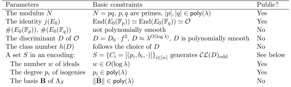
For convenience of the reader and for further reference, we provide in Figure4a summary of the pa-rameters, with the basic constraints they should satisfy, and whether they are public or hidden. The correctness and efficiency reasons behind these constraints will be detailed in the coming paragraphs, whereas the security reasons will be explained in§5.

Parameter generation. The parameter generation algorithmGen(1λ_{) takes the security}

param-eter 1λ as input, first chooses a non-maximal order O of an imaginary quadratic field as follows:

1. Select a square-free negative integerD0≡1 mod 4 as the fundamental discriminant, such that

(21)

Parameters Basic constraints Public? The modulus N N =pq,p, q are primes,|p|,|q| ∈poly(λ) Yes The identityj(E0) End(E0(Fp))'End(E0(Fq))' O Yes

#(E0(Fp)), #(E0(Fq)) not polynomially smooth No

The discriminant Dof O D=D0·f2,D≈λO(logλ),Dis polynomially smooth No The class number h(D) follows the choice ofD No A setS in an encoding: S={Ci= [(pi, bi,·)]}_i_∈[_w_]generates CL(D)odd See below

The numberw of ideals w∈O(logλ) Yes

The degree pi of isogenies pi ∈poly(λ) Yes

The basis B of ΛS kB˜k ∈poly(λ) No

Figure 4: Summary of the choices of parameters in the basic setting.

2. Choose k = O(log(λ)), and a set of distinct polynomially large prime numbers {fi}i∈[k] such

that the odd-part offi− D_f_i0

is square-free and not divisible byh(D0). Letf =Qi∈[k]fi.

3. SetD=f2D0. Recall from Eqn. (1) that

h(D) = 2· h(D0)

w(D0)

Y

i∈[k]

fi−

D0

fi

(5)

LetCL(O)_odd be the odd part of CL(O), h(D)odd be largest odd factor of h(D). Note that due to the choices ofD0 and {fi},CL(O)oddis cyclic, and we have|D|, h(D)odd ∈λO(logλ). The group with infeasible inversionGis then CL(O)odd with group orderh(D)odd.

We then sample the public parameters as follows:

1. Choose two primes p, q, and elliptic curves E0,Fp, E0,Fq with discriminant D, using the CM

method (cf. [LZ94] and more).

2. Check whetherpandqare safe RSA primes (if not, then back to the previous step and restart). Also, check whether the number of points #(E0(Fp)), #(E0(Fq)), #( ˜E0(Fp)), #( ˜E0(Fq)) (where

˜

Edenotes the quadratic twist ofE) are polynomially smooth (if yes, then back to the previous step and restart). p,q and the number of points should be hidden for security.

3. Set the modulusN asN :=p·q and letj0=CRT(p, q;j(E0,Fp), j(E0,Fq)). Let j0 represent the

identity ofG.

Output (N, j0) as the public parameterPP. Keep (D, p, q) as the trapdoorτ (Dand the group order ofGshould be hidden for security).

The sampling algorithm and the group operation of the composable encodings. Next we provide the definitions and the algorithms for the composable encoding.

Definition 4.2(Composable encoding). Given a factorization ofxasQw

i=1C

ei

i , wherew∈O(logλ); Ci = [(pi, bi,·)]∈G, ei∈N, for i∈[w]. A composable encoding of x∈G is represented by

(22)

where all the primes in the list L= (p1, ..., pw) are distinct; for each i∈[w], Ti ∈(Z/NZ)ei is a list

of thej-invariants such that ji,k =Cik∗j0, for k∈[ei].

The degree of an encodingenc(x) is defined to be d(enc(x)) :=Qw

i=1p

ei

i .

Notice that the factorization of x = Qw

i=1C

ei

i has to satisfy ei ∈ poly(λ), for all i ∈ [w], so as to

ensure the length ofenc(x) is polynomial. Looking ahead, we also require each pi, the degree of the isogeny that represents theCi-action, to be polynomially large so as to ensure Algorithm4.3 in the

encoding sampling algorithm and Algorithm4.9in the extraction algorithm run in polynomial time.

The composable encoding sampling algorithm requires the following subroutine:

Algorithm 4.3. act(τ, j, C) takes as input the trapdoor τ = (D, p, q), a j-invariant j∈_Z/NZ, and

an ideal class C∈ CL(O), proceeds as follows: 1. Let jp =j mod p, jq=j mod q.

2. Compute j_p0 :=C∗jp ∈Fp,jq0 :=C∗jq ∈Fq.

3. Output j0 :=CRT(p, q;j_p0, j_q0).

Algorithm 4.4(Sample a composable encoding). Given as input the public parameterPP= (N, j0), the trapdoor τ = (D, p, q), and x ∈ _G, TrapSam(PP, τ, x) produces a composable encoding of x is sampled as follows:

1. Choose w∈O(logλ) and a generation setS ={Ci = [(pi, bi,·)]}_i_∈[_w_]⊂G.

2. Sample a short basis B (in the sense that kB˜k ∈poly(λ)) for the relation lattice ΛS:

ΛS:=

 



y|y∈Zw, Y

i∈[w]

Cyi

i = 1G

 



. (6)

3. Given x, S, B, sample a short vectore∈ {poly(λ)∩_N}w such that x=Q

i∈[w]C

ei

i .

4. For alli∈[w]: (a) Let ji,0 :=j0.

(b) For k= 1 to ei: compute ji,k :=act(τ, ji,k−1, Ci).

(c) Let Ti := (ji,1, ..., ji,ei).

5. Let L∈Nw be a list where the ith entry of L ispi.

6. Output the composable encoding of x as

enc(x) = (L;T1, ..., Tw) = ((p1, ..., pw); (j1,1, ..., j1,e1), ...,(jw,1, ..., jw,ew)).

Remark 4.5(Thinking of each adjacent pair ofj-invariants as an isogeny). In eachTi, each adjacent

pair of thej-invariants can be thought of representing an isogenyφthat corresponds to the ideal class

Ci = [(pi, bi,·)]. Over the finite field, Ci can be explicitly recovered from an adjacent pair of the j

-invariants and pi (cf. Remark 2.3). Over Z/NZ, the rational polynomial of the isogeny φ can be

recovered from the adjacent pair of the j-invariants and pi (cf. Proposition 3.9), but it is not clear how to recoverbi in the binary quadratic form representation of Ci.

Remark 4.6(The only stateful step in the sampling algorithm). Recall that the basic setting assumes the encoding algorithm is stateful, where the state records the prime factors of the degrees used in the existing composable encodings. The state is only used in the first step to choose the{pi} of the ideals

(23)

Group operations. Given two composable encodings, the group operation is done by simply concatenating the encodings if their degrees are coprime, or otherwise outputting “failure”.

Algorithm 4.7. The encoding composition algorithm Compose(PP,enc(x),enc(y)) parses enc(x) = (Lx;Tx,1, ..., Tx,wx),enc(y) = (Ly;Ty,1, ..., Ty,wy), produces the composable encoding of x◦yas follows:

• If gcd(d(enc(x)), d(enc(y))) = 1, then output the composable encoding of x◦y as

enc(x◦y) = (Lx||Ly;Tx,1, ..., Tx,wx, Ty,1, ..., Ty,wy).

• If gcd(d(enc(x)), d(enc(y)))>1, output “failure”.

The canonical encoding and the extraction algorithm.

Definition 4.8 (Canonical encoding). The canonical encoding ofx∈_Gis x∗j0 ∈Z/NZ.

The canonical encoding of x can be computed by first obtaining a composable encoding of x, and then converting the composable encoding into the canonical encoding using the extraction algorithm. The extraction algorithm requires the following subroutine.

Algorithm 4.9 (The “gcd” operation). The algorithm gcd.op(PP, `1, `2;j1, j2) takes as input the

public parameter PP, two degrees `1, `2 and two j-invariants j1, j2, proceeds as follows:

• If gcd(`1, `2) = 1, then it computes the linear function f(x) = gcd(Φ`2(j1, x),Φ`1(j2, x)) over

Z/NZ, and outputs the only root off(x);

• If gcd(`1, `2)>1, it outputs ⊥.

Algorithm 4.10. Ext(PP,enc(x)) converts the composable encoding enc(x) into the canonical en-coding enc∗(x). The algorithm maintains a pair of lists (U, V), where U stores a list ofj-invariants

(j1, ..., j|U|),V stores a list of degrees where theith entry ofV is the degree of isogeny betweenji and ji−1 (when i= 1, ji−1 is the j0 in the public parameter). The lengths of U and V are always equal

during the execution of the algorithm.

The algorithm parsesenc(x) = (L;T1, ..., Tw), proceeds as follows:

1. Initialization: Let U :=T1, V := (L1, ..., L1) of length |T1|(i.e. copy L1 for |T1|times ).

2. For i= 2 tow:

(a) Set utemp:=|U|.

(b) For k= 1 to |Ti|:

i. Letti,k,0 be the kth j-invariant in Ti, i.e. ji,k;

ii. For h= 1 to utemp:

• If k= 1, compute ti,k,h:=gcd.op(PP, Li, Vh;ti,k,h−1, Uh);

• If k >1, compute ti,k,h:=gcd.op(PP, Li, Vh;ti,k,h−1, ti,k−1,h);

iii. Append ti,k,utemp to the list U, append Li to the list V.

(24)

j0 j1,1 j1,2 j1,3

j2,1

j2,2

j3,1

t2,1,1 t2,1,2 t2,1,3

t2,2,1 t2,2,2 t2,2,3

t3,1,1 t3,1,2 t3,1,3

t3,1,4

t3,1,5

` ` `

m

n

Figure 5: An example for the composable encoding and the extraction algorithm.

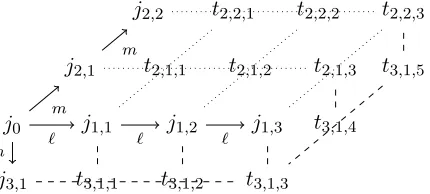
Example 4.11. Let us give a simple example for the composition and the extraction algorithms. Let `, m, n be three distinct polynomially large primes. Let the composable encoding of an element

y be enc(y) = ((`); (j1,1, j1,2, j1,3)), based on the factorization of y = C1e1 = [(`, b`,·)]3. Let the

composable encoding of an elementzbeenc(z) = ((m, n); (j2,1, j2,2),(j3,1)), based on the factorization

ofz=Ce2

2 ·C3e3 = [(m, bm,·)]2·[(n, bn,·)]1. Then the composable encoding of x=y◦z obtained from

Algorithm4.7 is enc(x) = ((`, m, n); (j1,1, j1,2, j1,3),(j2,1, j2,2),(j3,1)).

Next we explain how to extract the canonical encoding ofxfromenc(x). In Figure5, thej-invariants in enc(x) are placed on the solid arrows (their positions do not follow the relative positions on the volcano). We can think of each gcd operation in Algorithm 4.9 as fulfilling a missing vertex of a parallelogram defined by three existing vertices.

When runningExt(PP,enc(x)), the list U is initialized as (j1,1, j1,2, j1,3), the list V is initialized as

(`, `, `). Let us go through the algorithm for i= 2 and i= 3 in the second step.

• When i= 2, utemp equals to |U|= 3. The intermediate j-invariants {t2,k,h}_k∈[|T2|],h∈[utemp] are

placed on the dotted lines, computed in the order oft2,1,1, t2,1,2, t2,1,3, t2,2,1, t2,2,2, t2,2,3. The

list U is updated to(j1,1, j1,2, j1,3, t2,1,3, t2,2,3), the list V is updated to(`, `, `, m, m)

• When i= 3, utemp equals to |U|= 5. The intermediate j-invariants {t3,1,h}_h∈[utemp] are placed

on the dashed lines, computed in the order of t3,1,1, ..., t3,1,5. In the end, t3,1,5 is appended to

U, n is appended toV.

The canonical encoding ofx is then t3,1,5.

On correctness and efficiency. We now verify the correctness and efficiency of the parameter generation, encoding sampling, composition, and the extraction algorithms.

To begin with, we verify that the canonical encoding correctly and uniquely determines the group element in CL(O). It follows from the choices of the elliptic curves E0(Fp) and E0(Fq) with

End(E0(Fp))'End(E0(Fq))' O, and the following bijection once we fixE0:

CL(O)→EllO(k), x7→x∗j(E0(k)), fork∈ {Fp,Fq}

Next, we will show that generating the parameters, i.e. the curves E0,Fp, E0,Fq with a given

fun-damental discriminant D0 and a conductor f = Qikfi, is efficient when |D0| and all the factors of f are of polynomial size. Let u be an integer such that f | u. Choose a p and tp such that