A New Type Of Node Split Rule For Decision Tree Learning

(1)

Volume 4, No.8 , May-June 2013

International Journal of Advanced Research in Computer Science

RESEARCH PAPER

Available Online at www.ijarcs.info

A New Type Of Node Split Rule For Decision Tree Learning

C. Sudarsana Reddy

Department of Computer Science and Engineering, S.V. University College of Engineering,

S.V. University, Tirupati, India [email protected]

Dr. V. Vasu Department of Mathematics,

S.V. University, Tirupati, India [email protected]

B. Kumara Swamy Achari Department of Mathematics, S.V. University, Tirupati, India [email protected]

Abstract: A new type of node split rule for decision tree learning is proposed. This new type of node splitting rule is named as Sudarsana Reddy Node Split Rule (SRNSR). SRNSR is very easy to compute. It involves only finding the sum of logarithmic values of non-zero class counts of values of each attribute. The attribute with the highest logarithmic sum value will be selected as the best node split attribute.

SRNSR is compared with most important and popular node split attribute rules (measures) and its performance is noticed better than the best node split attribute measures. We have proved that decision trees constructed by using SRNSR node split rule are more efficient and robust. SRNSR decision trees are balanced, simpler, smaller, stable, and safe and more generalize decision trees.

We propose a new type of node splitting rule called Sudarsana Reddy Node Split Rule (SRNSR) for decision tree classifier construction. SRNSR improves decision tree classifier construction efficiency. Multi-way splits are applied for categorical attributes and binary splits are applied for numerical attributes.

Finding best splitting attribute is an important task in decision tree learning. Also it is well known fact that there is no single splitting attribute rule that gives best performance results for all the problem domains.

Keywords: Decision trees, split attribute, Sudarsana Reddy Node Split Rule (SRNSR), node split rules, classification, data mining, machine learning.

I. INTRODUCTION

Data mining is a method of finding new relationships among attributes in the large training data sets. Decision trees are most important and most popular data classification tools in data mining, machine learning and pattern recognition applications. In many real world applications decision trees are widely used for classification. A critical problem in building decision trees is the best attribute selection measure problem. We always prefer to produce small decision trees with high classification accuracy.

The present paper proposes an easy and a new type of decision tree node splitting rule. This new type of node splitting rule is named as Sudarsana Reddy Node Split Rule (SRNSR). SRNSR is very easy to compute and it involves only simple additions and logarithmic calculations of class counts of values of each attribute.

Decision tree induction is the learning of decision trees from class-labeled training tuples [1]. During decision tree construction at each internal node, class counts of values of each attribute are computed. The attribute with the highest sum of logarithmic class counts of values of each attribute is selected as best split attribute at the current node.

In this paper, we study the problem of constructing decision tree classifiers using training data sets containing categorical (nominal) as well as numerical (continuous) attributes. Our goal is to construct an efficient decision tree classifier using a new split attribute rule that is very simple and easy to understand and implement. Computational cost of new split attribute rule is very less.

The main goal of node split rule is to find the attribute that “best” divides the training tuples into subsets. The main advantage of our new attribute splitting rule, SRNSR, is that its calculations require only the distribution of the class values for each attribute. The attribute with maximum sum of logarithmic values of class counts of values of each attribute is selected as the best or optimal split attribute.

When decision trees are used for classification they are called classification trees [2]. Different types of split attribute rules are used for decision tree learning. Gain, Gain Ratio, Gini Index, Twoing and miss classification are the most important split attribute measures. All these measures are defined in terms of the reduction of impurity from the parent node to the child nodes. The goodness of a split attributes increases as the reduction of impurity increases.

A classification rule will be expressed as a decision tree [4]. The term continuous is used in the literature to indicate both real and integer valued attributes [5]. Continuous valued attributes must be discretized prior to attribute selection [5]. Since the split point must occur on a boundary we only need to evaluate boundary points between classes instead of evaluating possibly all g – 1 candidate split points for a given g number of tuples [5].

II. RELATED WORKS

(2)

a. Information rules

b. Distance measures rules and c. Dependence measures rules

There exist many attribute selection rules that do not clearly belong to any category in Ben Bassat’s taxonomy [3]. No split attribute selection rule is consistently superior to the others.

Classification is an important data mining problem. Impurity based split attribute selection methods are widely used and very popular. Also studies have shown that this class of split attribute selection methods produces decision trees with high predictive accuracy. Most previous work in the database literature uses impurity based split attribute selection methods. Impurity based split attribute selection methods calculate the splitting criterion by minimizing the concave impurity functions.

Decision trees are valuable tools for description, classification and generalization of data [3]. Greedy top-down construction is the most commonly used method for decision tree construction. A decision tree is constructed from a training data set consisting of tuples. Each tuple is completely described by a set of attributes and a class label. The task of constructing a decision tree from the training data set is called decision tree induction [2]. Discrimination is the process of deriving classification rules from classified tuples and classification is the process of applying the rules to new tuples of unknown class labels [3].

Number of tuples that are correctly classified by a decision tree classifier is known as its accuracy, whereas the number of misclassified tuples is the error. The accuracy of a classifier on a given test set is the percentage of test set tuples that are correctly classified by the classifier [1]. The accuracy of a classifier refers to the ability of a given classifier to correctly predict the class label of new or previously unseen data [1].

Minimum description length (MDL) is also used for deciding which attribute splits to prefer over others. Information Gain and Gini index are concave [3].

The total number of misclassified tuples has been explored as attribute selection criteria by many authors. Two examples under this category are - sum minority and inaccuracy [3]. Additional tricks are needed to make this measure useful.

Max minority (Maximum of the number of misclassified tuples on two sides of a binary split) and sum of impurities (which assigns an integer to each class and measures the variance between class numbers in each partition).

Most of the attribute evaluation measures assume no knowledge of the probability of the training data tuples. The optimal decision rule at each decision tree node is used. A rule that minimizes the overall error probability is considered assuming that complete probabilistic information about the data is known.

A hard split divides the data into mutually exclusive partitions [3]. A soft split, on the other hand, assigns a probability that each tuple belongs to a partition, thus allowing tuples to belong to multiple partitions. C4.5 uses a simple form of soft splitting [3].

III. PROBLEM STATEMENT

There exist many node split rules or measurement techniques for selecting the best split attribute during

decision tree induction. All these rules or measures are defined in terms of the reduction of impurity from the parent node to the child nodes. Reduction of impurity is the difference between impurity of the parent node before split and sum of the impurities of its child nodes after split.

Reduction of impurity = Impurity of parent node before split – Sum of impurities of child nodes after split.

Information Gain (or Gain), Gain Ratio, Gini Index, Twoing are the most important and popular rules of node splitting attribute rules. Computational complexity of these rules is very high because many multiplications, divisions and square operations are needed.

The present study proposes a new node split rule or measure called Sudarsana Reddy Node Split Rule (SRNSR) for selecting the best split attribute during decision tree construction. This new rule or measure is very easy to compute and understand. Computational complexity of this rule is very less. It overcomes many of the problems of existing node split rules or measures for selecting the best split attribute during decision tree induction.

IV. EXISTING NODE SPLIT RULES

The problem of building a decision tree can be expressed recursively. Initially the selected split attribute rule is applied to each attribute of the training data set and then best split attribute is selected and placed at the root node. Tuples at the root node are divided into subsets based on the categorical values of the split attribute or if the split attribute is numerical then tuples at the root node are divided into two subsets based on the best value of best split attribute. Same process is repeated for all internal nodes.

Existing split attribute measures for selecting the best split attributes:

Information Gain (or Gain), Gain Ratio, Gini Index, Twoing are the most important rules of node splitting attribute rules. Each rule has its own advantages and disadvantages. No one rule is best in all cases.

A. Information Gain (or Gain):

Gain is predominantly used as a measure for selecting the best split attribute. Information gain is the most popularly used node split rule or measurement technique for selecting the best split attribute. Its main disadvantage is that it deviates to select attributes with a large number of distinct values. This deviation decreases the performance and accuracy of the learned decision tree classifier.

The attribute with the maximum information gain is selected as a split attribute. Information gain is a popular way to select best split attribute.

Gain = Information (Parent) – Sum of information details of all children.

B. Gain Ratio:

The information gain measure is biased toward tests with many outcomes [1]. That is, it prefers to select attributes having a large number of values [1]. The attribute with the maximum gain ratio is selected as the splitting attribute [1].

(3)

C. Gini Index

The main disadvantage of the Gini index is that it tries to put tuples of the majority class into one subset and the remaining tuples into the other subset.

The Gini index is used in CART [1]. The Gini index measures the impurity of D, a data partition or set of training tuples, as

Where pi is the probability that a tuple in D belongs to

class Ci and is estimated by . The sum is computed over m classes. The Gini index considers a binary split for each attribute [1]. When considering a binary split, we compute a weighted sum of the impurity of each resulting partition [1]. For example, if a binary split on A partitions D into D1 and

D2, the Gini index of D given that partitioning is

D. Twoing rule:

An alternative measure of node impurity is the twoing index

where L and R refer to the left and right sides of a given split respectively, and p(i|t) is the relative frequency of class

i at node t. Twoing attempts to segregate data more evenly than the Gini rule, separating whole groups of data and identifying groups that make up 50 percent of the remaining data at each successive node.

V. PROPOSED NODE SPLIT RULE

The decision tree classifier is built recursively in a top-down manner, starting from the root. At each node both categorical and numerical attributes are considered. For each node, attribute split rule is applied and the sum of logarithmic values of class counts of all the values of each attribute are computed. The attribute with the highest logarithmic sum value is selected as the best split attribute. The node is assigned that best split attribute. If the best split attribute is categorical then tuples at the current node are divided into subsets based on the distinct values of the best attribute. If the best attribute is numerical attribute then tuples at the current node are divided into two (binary) subsets based on the best value of the best split attribute. Same process is repeated at each internal node.

Decision tree is a classification tool. Decision trees are constructed based on the node split attribute rules. Split attribute rules are used to select best split attribute at each internal node of the decision tree.

A. Information Gain (or Gain):

The main disadvantage or bias of the Gain rule is that it tries to select attributes with a large number of distinct values, this leads to degraded performance of the learned decision tree classifies.

Our new approach, SRNSR, for selecting the best split attribute overcomes this problem by separating the training

tuples into large subsets and without any bias towards the selection of attributes with a large number of distinct values. Additional advantage of our approach is that the height of the resultant decision tree is very small because our approach tries to divide training tuples into larger groups as much as possible.

B. Gain Ratio:

The main disadvantage of the Gain Ratio is that sometimes split-info value becomes zero or very small, which leads to infinite or undefined or very large Gain Ratio Value.

In our new splitting rule approach, SRNSR, just we are using small number of additions and logarithmic values of class counts. There are no multiplications, divisions and square operations at all. So, our approach overcomes this problem also. Hence, our approach is far better than Gain Ratio.

Our new approach, SRNSR, not only overcomes the disadvantages of Gain, Gain Ratio but also produces smaller and much faster decision tree classifiers and at the same time maintains the high classification accuracies.

Our approach is very simple and elegant attribute splitting rule or measure for selecting the best split attribute during decision tree learning. Our approach is applied to training data sets containing categorical attributes. Same approach can be applied to continuous or numerical attributes also.

C. Gini Index:

In Gini index operations like multiplications, divisions and squares are needed. In our new split attribute approach, SRNSR, only additions and logarithmic operations are needed.

D. Twoing Rule

In Twoing rule also many multiplications, divisions, and square operations are needed. Hence, new SRNSR approach is very efficient than Twoing rule.

We propose a new type of node splitting rule named Sudarsana Reddy Node Split Rule (SRNSR). It is very simple and easy to understand, implement and compute. It involves only simple calculations. It overcomes many of the problems in the existing attribute splitting rules or measures.

E. Decision Tree construction example using our

new splitting rule, Sudarsana Reddy Node Splitting Rule (SRNSR):

(4)

We have already proposed a new type of node splitting rule called Sudarsana Reddy product rule (SR-product rule) for decision tree node splitting during the construction of decision tree learning. But the main disadvantage of SR-product rule is that the SR-product value becomes very large for very large training data sets. To overcome this problem in this paper we propose a new type of node split rule called SRNSR logarithmic rule.

In this paper we have calculated the results for both the node split rules - Sudarsana Reddy product rule (SR-product rule) and Sudarsana Reddy Node Split Rule (SRNSR) or SR- logarithmic rule for compatibility.

Table2. Age attribute class count values

Age Buys_Computer

Yes No

Youth 2 3

Middle_aged 4 0

Senior 3 2

Age attribute has 3 distinct values – Youth, Middle_aged, and senior. Non-zero class count values of age attribute are shown in Table2

Product of non-zero class count values of age attribute = product(Age) = 2 x 3 x 4 x 3 x 2 = 144.

product(Age) = 144.

Sum of logarithmic values of non-zero class count values of age attribute = log 2 + log 3 + log 4 + log 3 + log 2 That is,

logsum(Age) = log 2 + log 3 + log 4 + log 3 + log 2 logsum(Age) = 0.301030 + 0.477121 + 0.602060 + 0.477121 + 0.301030.

[image:4.595.62.254.440.498.2]

logsum(age) = 2.158362

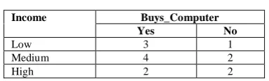
Table 3. Income attribute class count values

Income Buys_Computer

Yes No

Low 3 1

Medium 4 2

High 2 2

Income attribute has 3 distinct values – Low, Medium, and High. Non-zero class count values of income attribute are shown in Table3.

Product of non-zero class count values of income attribute is equal to = product(Income) =3x1x4x 2x 2x2= 96.

product(Income) = 96.

Sum of logarithmic values of non-zero class count values of income attribute =log 3 + log 1 + log 4 + log 2 + log 2+log 2 That is, logsum(Income)=

log 3 + log 1 + log 4 + log 2 + log 2 + log 2 logsum(Income) = 0.477121 + 0 + 0.602060 + 0.301030 + 0.301030 + 0.301030.

logsum(Income) = 1.982271

Table4. Student attribute class count values

Student Buys_Computer

Yes No

Yes 6 1

No 3 4

Student attribute has 2 distinct values – Yes, and No. Non-zero class count values of student attribute are shown in Table4.

Product of non-zero class count values of student attribute is equal to = product(Student) = 6 x 1 x 3 x 4 = 72.

product(Student) = 72.

Sum of logarithmic values of non-zero class count values of student attribute = log 6 + log1 + log 3 + log 4

That is,

logsum(Student) = log 6 + log1 + log 3 + log 4

logsum(Student) = 0.778151 + 0.477121 + 0 + 0.602060

logsum(Student) = 1.857332

Table5. Credit_Rating class count values

Credit_Rating Buys Computer

Yes No

Fair 6 2

Excellent 3 3

Credit_Rating attribute has 2 distinct values – Fair, and Excellent. Non-zero class count values of Credit_Rating attribute are shown in Table5.

Product of non-zero class count values of Credit_Rating attribute = product(Credit_Rating) = 6 x 2 x 3 x 3 = 108.

product(Credit_Rating) = 108.

Sum of logarithmic values of non-zero class count values of Credit_Rating attribute = log 6 + log 2 + log 3 + log 3 That is, logsum(Credit_Rating)= log 6 + log 2 + log 3+log 3 logsum(Credit_Rating) = 0.778151 + 0.301030 + 0.477121 + 0.477121.

logsum(Credit_Rating) = 2.033423

Sudarsana Reddy product rule (SR-product rule) calculations are-maximum(144, 96, 72, 108) = 144. Note if any class count is zero then it must be taken as 1; otherwise the product becomes zero.

Here maximum product(Age) value is 144. Hence, split attribute is Age.

Sudarsana Reddy Node Split Rule (SRNSR) calculations are used in finding the largest logarithmic value.

That is,

maximum(2.158362,1.982271,2.857332,2.033423)=2.15836

Here Age has highest logsum value. So split attribute is Age.

In this paper we consider our new type of node splitting rule called Sudarsana Reddy Node Splitting Rule (SRNSR) during decision tree construction and we use only highest logsum value for finding best split attribute.

Initially the root node contains all the tuples and age is the best splitting attribute in the root node. These tuples must be divided into groups based on the distinct values of the age attribute. Age attribute has three distinct values, so training data set shown in Table1 is divided into three partitions which are shown in Table6, Table12 and Table13.

Table6. Tuples corresponding to age = “Youth”

Income Student Credit_Rating Buys_Computer

High No Fair No

High No Excellent No

Medium No Fair No

Low Yes Fair Yes

Medium Yes Excellent Yes

Table7. Income attribute class count values

Yes No

High 0 2

Medium 1 1

(5)

In Table6 Income attribute has 3 distinct values–Low, Medium, and High. Non-zero class count values of income attribute are shown in Table7.

Product of non-zero class count values of income attribute is = product(Income) = 2 x 1 x 1 x 1 = 2

Sum of logarithmic values of non-zero class count values of income attribute = log 2 + log 1 + log 1 + log 1

That is, logsum(Income) = log 2 + log 1 + log 1 + log 1 logsum(Income) = 0.301030 + 0 + 0 + 0 = 0.301030

logsum(Income) = 0.301030

Yes No

Yes 2 0

No 0 3

Student attribute has 2 distinct values – Yes and No. Non-zero class count values of income attribute are shown in Table8

Product of non-zero class count values of student attribute is = product(Student) = 2 x 3 = 6

Sum of logarithmic values of non-zero class count values of income attribute = log 2 + log 3

That is, logsum(Student) = log 2 + log 3

logsum(Student) = 0.301030 + 0.477121 = 0.778151

logsum(Student) = 0.778151

Table9. Credit_Rating attribute class count values

Credit_Rating Buys_Computer

Yes No

Excellent 1 1

Fair 1 2

Credit_Rating attribute has 2 distinct values – Excellent and Fair. Non-zero class count values of Credit_Rating attribute are shown in Table 9

Product of non-zero class count values of Credit_Rating attribute is equal to = product(Credit_Rating)=1x1x1x2 = 2

Sum of logarithmic values of non-zero class count values of Credit_Rating attribute = log 2

That is, logsum(Credit_Rating) = log 2 logsum(Credit_Rating) = 0.301030

logsum(Credit_Rating) = 0.301030

Here, maximum product is 6, so best split attribute is Student according to SRNSR-product rule.

Here, maximum(0.301030, 0.778151, 0.301030) = 0.778151. Hence, best split attribute is Student according to SRNSR-logarithmic rule. Hence, Table6 is divided into Table10 and Table11. Now Table10 and Table11 need not to classify further because all tuples belongs to the same class. Hence, Table10 and Table11 are leaf nodes.

Table10. Tuples corresponding to student = “No”

Income Credit_Rating Buys_Computer

High Fair No

High Excellent No

Medium Fair No

Table11. Tuples corresponding to student = “Yes”

Income Credit_Rating Buys_Computer

Low Fair Yes

Medium Excellent Yes

Table12. Tuples corresponding to age = “Middle_aged”

High No Fair Yes

Low Yes Excellent Yes

Medium No Excellent Yes

High Yes Fair Yes

All the tuples in Table12 have the same class label, so no need to further classify and hence it becomes a leaf node.

Table13. Tuples corresponding to age = “Senior”

Medium No Fair Yes

Low Yes Fair Yes

Medium Yes Fair Yes

Medium No Excellent No

Table14. Income attribute class count values

Yes No

Medium 2 1

Low 1 2

In the Table13 Income attribute has 2 distinct values - Low and Medium. Non-zero class count values of Income attribute are shown in Table14

Product of non-zero class count values of income attribute is = product(Income) = 2 x 1 x 1 x 2 = 4

Sum of logarithmic values of non-zero class count values of income attribute = log 2 + log 1 + log 1 + log 2

That is, logsum(Income) = log 2 + log 1 + log 1 + log 2 logsum(Income) = 0.301030 + 0 + 0 + 0.301030 = 0.602060

Yes No

No 1 1

Yes 2 1

Student attribute has 2 distinct values: No and Yes. Non-zero class count values of Student attribute are shown in Table15

Product of non-zero class count values of Student attribute is = product(Student) = 1 x 1 x 2 x 1 = 2

Sum of logarithmic values of non-zero class count values of Student attribute = log 1 + log 1 + log 2 + log 1

That is,

logsum(Student) = log 1 + log 1 + log 2 + log 1 logsum(Student) = 0 + 0 + 0.301030 + 0 = 0.301030

logsum(Student) = 0.301030

Table16. Product 3x2 = 6

Credit_Rating Buys_Computer

Yes No

Fair 3 0

Excellent 0 2

In the Table13 Credit_Rating attribute has 2 distinct values: Fair and Excellent. Non-zero class count values of Credit_Rating attribute are shown in Table16

(6)

Sum of logarithmic values of non-zero class count values of income attribute = log 3 + log 2

That is,

logsum(Income) = log 3 + log 2

logsum(Income) = 0.477121 + 0.301030 = 0.778151

[image:6.595.42.275.575.751.2]

Here, Credit_Rating attribute has the highest logarithmic value. So, best split attribute for the training data tuples in the Table13 is Credit_Rating. Hence, Tuples in Table13 are partitioned into Table17 and Table18. Both Table17 and Table18 are leaf nodes. So, no need to further partition them.

Table 17. Tuples corresponding to Credit_Rating = “Fair”

Income Student Buys_Computer

Medium No Yes

Low Yes Yes

Medium Yes Yes

Table18. Tuples corresponding to Credit_Rating = “Excellent”

Income Student Buys_Computer

Low Yes No

Medium No No

VI. EXPERIMENTAL RESULTS

We have experimentally verified that our new rule called Sudarsana Reddy Node Split Rule (SRNSR) works well and it is the most efficient method for dividing the tuples at the current node into subsets. SRNSR tries to divide set of tuples in the internal node into balanced subsets of tuples. Experimentally we have compared decision trees constructed using already available rules and decision trees constructed using our new rule SRNSR.

VII. CONCLUSIONS

A. Contributions:

A new type of node split rule called Sudarsana Reddy Node Split Rule (SRNSR) or SR-logarithmic rule for decision tree induction is proposed and verified experimentally by constructing a decision tree classifier using already existing node split rules and our new split attribute rule, SRNSR (SR-logarithmic rule). Experiments have shown that SRNSR is computationally most efficient and very easy to implement. SRNSR is very simple, easy to compute and involves only simple additions and logarithmic calculations.

B. Limitations:

Ours SRNSR is efficient for categorical attributes and the efficiency of our new split attribute rule must be improved for numerical split attributes.

C. Suggestions for feature work:

Special techniques are needed to increase the scalability of decision tree learning using our new split attribute rule, SRNSR.

VIII. REFERENCES

[1]. Jiawei Han, Micheline Kamber, Data Mining: Concepts and Techniques, Morgan Kaufmann, second edition, 2006. pp. 285–292

[2]. Introduction to Machine Learning Ethem Alpaydin PHI MIT Press, second edition. pp. 185–188

[3]. Automatic Construction of decision Trees from data, SREERAMA K. MURTHY: A Multi-Disciplinary Survey

[4]. J.R. Quinlan, “Induction of Decision Trees,” Machine Learning, vol. 1, no. 1, pp. 81-106, 1986.

[5]. U.M. Fayyad and K.B. Irani, “On the Handling of Continuous –Valued Attributes in Decision tree Generation”, Machine Learning, vol. 8, pp. 87-102, 1996.

[6] C. Sudarsana Reddy, Dr. V. VASU, B. Kumara Swamy

Achari, “Decision Trees For Training Data Sets Containing

Numerical Attributes with Measurement Errors”,

International Journal of Advanced Research in Computer