Statistical and Artificial Neural Network Based Modeling of Parallel Job Scheduling Algorithms

Volume 2, No. 4, July-August 2011

International Journal of Advanced Research in Computer Science

RESEARCH PAPER

Available Online at www.ijarcs.info

Statistical and Artificial Neural Network Based Modeling of Parallel Job Scheduling

Algorithms

Amit Chhabra*

Assistant Professor, Department of Computer Science & Engineering, Guru Nanak Dev University,

Amritsar, India [email protected]

Gurvinder Singh

Associate Professor, Department of Computer Science & Engineering, Guru Nanak Dev University,

Amritsar, India [email protected]

Abstract: The prime applicability of parallel space-sharing job scheduling algorithms in PC-cluster is to schedule jobs and efficiently allocate cluster's processors to the jobs to achieve performance objective viz. minimized average turnaround time (ATT). This paper demonstrates the use of the two-phase strategy based on the Response Surface Methodology (RSM) approach of Design of Experiments (DOE) and Artificial Neural Networks (ANN) for modeling the performance of parallel space-sharing job scheduling algorithms particularly Largest Job First (LJF) algorithm. In the first phase DOE based statistical-mathematical techniques helps in identifying, ranking and modeling the significant independent scheduling process variables affecting the ATT based output values with minimal cost involved in terms of experimental runs, money and time. RSM based regression analysis helps to fit second-order quadratic empirical model equation for output metric ATT involving

main and interaction effects terms of scheduling process variables. High values of coefficient of determination R2, adjusted R2 and insignificant

lack of fit represent the goodness of fit of the model to accurately model the ATT values. In the second phase ANN model for ATT is developed using the experimental data passed from DOE phase to validate the RSM based model predictions. The two-phase modeling strategy tends to combines the advantages of RSM and ANN approaches.

Keywords: PC-cluster, Largest job first, Design of experiments, Response surface methodology, Average turnaround time, Artificial neural networks

I. INTRODUCTION

Virtual local area network (VLAN) based PC-cluster [1]-[4] are gaining momentum due to progressive technological advancements in the speed of requisite commodity hardware viz. microprocessors as well as networking technologies and easily availability of commonly used software (both open source and proprietary). Parallel space-sharing job scheduling algorithms try to assign a distinct partition (subset) of processors of PC-cluster’s processor-pool to the job selected by the scheduler. Jobs can run concurrently on the allocated partition of processors but no processor is concurrently assigned to more than one job. These job scheduling algorithms are involved in decision making regarding selection of a job from the set of competing jobs as well as allocating processors to the selected job. Program based machine partitioning technique [5,6] is used in the present study, in which the partitions of processors are created for individual applications based on their size at the time of their servicing i.e. scheduling time.

Scheduling algorithms like First Come First Serve (FCFS), Fit Processors First Served(FPFS) and Largest Job First (LJF) are mostly used for batch job scheduling [7] in space-shared clusters. In traditional LJF scheduling algorithm [8,9] queued jobs in the ready FIFO queue are sorted in descending order according to their job sizes so that the largest job will have the chance to acquire the required number of processors for execution. The sole job information known to the LJF scheduler at the time of arrival of the job is the job size i.e. number of processors requested by the job. Rigid [10] class of data-parallel jobs is considered in the present work. The behavioral

characteristic of a rigid kind of parallel job is that it will be selected by the LJF scheduler only if there are enough processors (equal to the job size) available to execute the job. In case the desired numbers of processors are not available, the first job and the other subsequent jobs in the job queue must wait for the availability of desired number of processors.

Design of experiments (DOE) is a set of organized statistical techniques [19,20] for planning, designing, executing and analyzing the experiments in a way to achieve reasonable and objective conclusions effectively and proficiently. Response surface methodology (RSM) is a meta-modeling approach [21] of DOE, consisting of mathematical and statistical techniques aimed to be used in modeling, establishing and analyzing the relationships existing between process variables and the observed response. Experimental designs based on RSM approach tends to minimize the expenditure involved in terms of the number of experiments required, time and money for performance modeling and analysis of the observed response.

the feedforward ANNs (the most commonly used form of ANs).

Conventional performance evaluation studies [8,9] [11-18] of parallel job scheduling algorithms based on experimental measurement, analytical/theoretical modeling, simulation techniques are capable of showing the main effects corresponding to the variation of only one-factor-at-a-time (OFAT) on the observed output and are incapable of predicting the interaction i.e. combined effects on the output response resulting due to simultaneous variation of two process variables. An interaction exists between two input process variables when effect of one variable on the observed output depends upon the level of another variable. Also the OFAT approach does not expound which factors are mostly affecting the output.

In the first phase, DOE based RSM technique is helpful in investigating the relationship of independent scheduling process variables with the observed response using mathematical model equation. In the second phase, an ANN model is developed from the experimental data to model the scheduling process and also to validate the predictions done by the RSM based mathematical model. The advantage [28,29] of ANN over statistical methods is that it can approximate a wide range of statistical models without finding the empirical relationship between process variables in the form of complicated mathematical model. In case of ANN, the form of input-output mappings is determined during the learning process. In this way, ANNs are referred as model-free estimators. ANNs have generalization

capability to get acquainted with problems by means of training and after adequate training it offers great flexibility to solve unknown problems of the same class. On the other hand, ANNs fail to express the mathematical relationship of the input scheduling process variables with the output response to understand which process variable is more significantly affecting(either positively or negatively) the output. The proposed work tends to combine the advantages of the both RSM and ANN based approaches to model the performance of parallel space-sharing LJF scheduling algorithm.

II. MATERIALSANDMETHODS

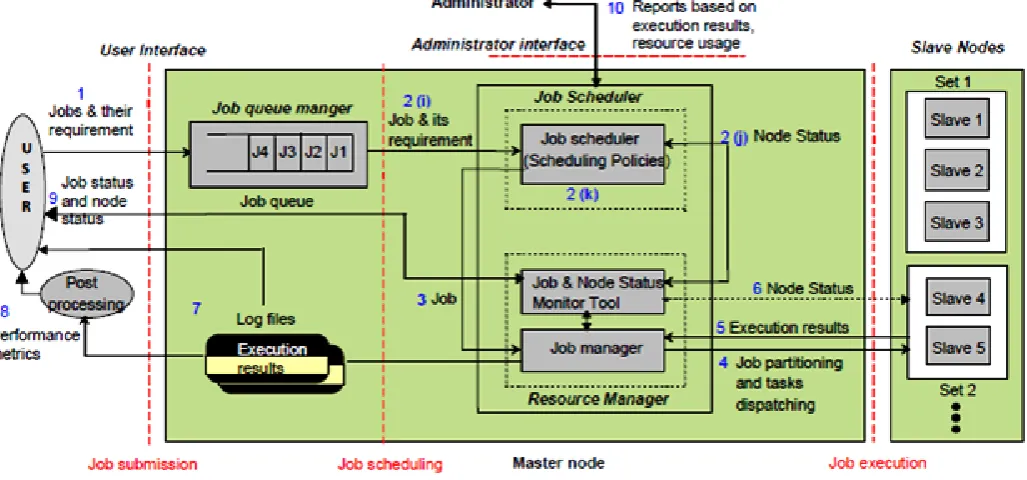
PC-cluster [22][23] is a pool of interconnected PCs working together as a single integrated computing resource with the help of single system image (SSI) functionality residing at cluster middleware layer. The SSI [24] represents the abstract view of cluster’s parallel and distributed computing system as a single unified computing resource to the user. The SSI of the cluster is realized with the help of a cluster distributed resource management system (RMS) of the cluster. A RMS[7][18][22] is developed in order to manage job scheduling related functionalities such as job submission, job scheduling, processor allocation, job execution and some other resource management activities. The generic architecture of the cluster distributed RMS system is shown in figure1.

Figure 1. Distributed resource management system and scheduling procedure

A. Experimental set-up and Procedure

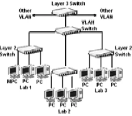
In the PC-cluster, VLAN based distribution switch (CISCO 3750 series) is used to connect twenty five networked computers available in the three different departmental computer laboratories. One of the nodes in the VLAN acts as master node (Pentium Core 2 duo with 1 GB RAM, Windows Server 2003 Enterprises Edition) and other twenty four PCs perform the role of slave or compute nodes (configured with Windows XP based Pentium IV 3.0 GHz and 512 MB RAM). Network switches used in the

entire job sizes are of the type 2n where n is a user specific integer within the range [1, 4] and size of PC-cluster falls in integer continuous range [16, 24].

Figure 2: Cluster network structure

Rigid parallel jobs are classified as small (number of processors required by job varies from 1-4) and large (number of processors required varies from 5-16). Workload submitted by the user to the job queue at time zero for scheduling consists of mixture of roughly 50% small and 50% large jobs. Master node with the help of key components of RMS viz. user interface & queue manager, job scheduler, job manager and resource manager helps cluster the user to submit, schedule and execute jobs. Slave nodes are only acting as computing nodes that are used for execution of the dispatched partitioned tasks of jobs as well as communicating the task execution results back to the master node.

The overall procedure for job submission, job scheduling and job execution is shown in fig. 1 using labeled numbers from step 1 to 10. User can able to submit the jobs along with information on the corresponding job sizes to job queue manager with the help of cluster user interface to the RMS at the master node in step 1.

A scheduling decision to select the job and consequent allocation of slave nodes is taken on the basis of the three kinds of information viz. job size details from step 2(i), node availability information obtained from job & node status monitoring tool of the resource manager at step 2(j) and type of scheduling policy at step 2(k). The selected job is forwarded to the job manager for dispatching in step 3. Job manager partitions the job into parallel tasks based on the number of slave nodes allotted to the job and dispatches the partitioned parallel tasks to the allocated slave nodes for execution. After the completion of the tasks at slave nodes, task execution results are sent back to the job manger module in step 5.

Another responsibility of the job manager is to merge the partial task execution results collected from various slaves to form the final result corresponding to the whole job. Final result and various real-time parameters related to job submission times, job completion times and job waiting times are stored in the text based log files. Job and node status is updated at step 5 and step 6 with the help of resource manager. This procedure from step 1 to 6 continues

till the job queue is empty. User can able to access these log files at master node console in step 7 with the help of cluster user interface. Results in terms of performance metric (ATT) of a job can be obtained as per (1) by doing standalone post-processing on the data collected from log files in step 8. Job and node status can be collected from resource manager module by the cluster user and the administrator at step 9 and 10 respectively.

Average turnaround time (ATT) represents the average completion time of a job and is defined as the time difference between the job submission time and the job completion (end) time averaged over all the jobs in the system. ATT is calculated using Eq. (1).

ATT = (1)

where N is the number of jobs with known job width characteristics, Job_SubmitTime(i) indicates the time when ith job is submitted to the job queuing system and Job_EndTime(i) denotes the time when ith job gets terminated.

B. Experimental Design and RSM Modeling Process

a. Selection of Process Variables and Response

First input parameter chosen for the scheduling system is schedule size which is the summation of job sizes of all the jobs in the workload and is denoted as ScheduleSize. Second input variable chosen in the model is the number of processors in the PC-cluster known as cluster size (ClusterSize). The chosen independent process variables (known as factors in DOE terminology) and observed output (known as response in DOE terms) along with their levels (variations) for modeling of observed response ATT values are shown in table 1.

Table I. Independent scheduling variables and their levels

Process

variables Symbols Levels (actual values)

ScheduleSize SS 66,100,134,168

ClusterSize CS 16 -24

b. Experimental Design and ATT Results

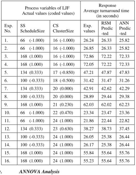
Based on RSM D-optimal coordinate exchange design, total of 16 experimental runs (table 2) in random order were conducted with various combinations of ScheduleSize and ClusterSize for LJF scheduling algorithm. This RSM based experimental design helps to minimize the number of experiments required to model their performance. Number of experiments required for scheduling process modeling using RSM design are 16 as compared to 36 in case of OFAT approach [25].

Table II. RSM based experimental design for LJF policy with experimental and model predictive response

Process variables of LJF Actual values (coded values)

Response Average turnaround time

(in seconds)

Exp. No.

SS ScheduleSize

CS ClusterSize

Exp. values

RSM Predic -ted

ANN Predic -ted

1. 66 (-1.000) 16 (-1.000) 26.24 26.33 25.82

2. 66 (-1.000) 16 (-1.000) 26.85 26.33 25.82

3. 168 (1.000) 16 (-1.000) 72.86 72.22 72.33

4. 168 (1.000) 16 (-1.000) 72.05 72.22 72.33

5. 134 (0.333) 17 (-0.850) 47.21 47.87 47.83

6. 100 (-0.333) 18 (-0.500) 31.42 31.47 31.26

7. 134 (0.333) 20 (0.000) 42.91 42.62 42.29

8. 100 (-0.333) 20 (0.000) 28.89 29.44 29.38

9. 168 (1.000) 21 (0.230) 62.03 62.02 62.23

10. 66 (-1.000) 22 (0.470) 23.34 23.47 23.36

11. 66 (-1.000) 24 (1.000) 21.86 22.44 22.82

12. 134 (0.333) 23 (0.630) 38.27 38.73 37.45

13. 100 (-0.333) 24 (1.000) 26.05 25.38 26.44

14. 100 (-0.333) 24 (1.000) 26.17 25.38 26.44

15. 168 (1.000) 24 (1.000) 55.84 55.64 55.76

16. 168 (1.000) 24 (1.000) 55.23 55.64 55.76

c. ANNOVA Analysis

Analysis of variance (ANNOVA) method is applied on the experimental data of the chosen quadratic model to determine the significance of models as well as the terms it contains. Insignificant terms (if any) in the models with p-value greater than 0.05 can be omitted to improve the models. Quadratic model fitting, ANNOVA based statistical analyses, regression coefficient estimation and visual result analyses by means of model diagnostic plots were carried out with the help of Design-Expert 8.0 software (StatEase Inc. USA)[26]. Statistics [19]-[20] that help to observe the goodness of fit of the model are high values of coefficient of determination R2, adjusted R2, predictive R2 and insignificant lack of fit. Lack of fit compares the residual error with the pure error obtained from replicated model points and it is not desirable feature. Adequate precision value is an indicator of signal to noise ratio (SNR) and SNR > 4 is desirable for the model to navigate the design space. d. Model adequacy Checking

In the selected polynomial model, model adequacy checking of the residuals was performed using various diagnostic plots [19][20][26]. Normality of residuals was checked using normal probability plot of studentized residuals. Plot of studentized residuals versus predicted values were diagnosed to check the constant error. Plot of externally studentized residuals was checked to see the presence of outliers i.e. influential values. Box-Cox plot was investigated for the power transformation suggestions to further improve the model. Power transformations were required in the cases when the max to min ratio of response is greater than 10 and/or presence of non-normality in the residual data.

e. Mathematical Model Equation Fitting

Output response ATT can be related to independent scheduling process variables using mathematical model equation. A second-order quadratic predictive model for ATT was described both in terms of coded values and the actual values of input factors with the help of method of least squares (MLS) based multiple regression equation given in Eq. (2).

y = β0 + i xi + ijxi xj + k xi 2_{+ ε}

(2) where y is known as the model predicted response, xi and xj are independent variables or factors, m is the number of independent factors, β0, βi, βk and βij are the regression

coefficients of intercept, first-order, second-order and interaction term respectively and ε is statistical random error.

f. Interpret and Validate the Results

The fitted coded equation as per Eq. (2) is useful for identifying the relative significance of the model factors in terms of their absolute effect on the model response by comparing the unitless estimated coefficients of the input factors. This significance analysis [4] cannot be done with the actual equation because its coefficients are scaled to accommodate the units of each factor and resulting equation can be biased towards larger scale factor. Coded variables are scaled between -1 to +1 to overcome this situation. In the end, interpolated predicted values of the quadratic model for LJF are validated against the additional actual experimentation results.

C. Artificial Neural Network (ANN) Modeling

ANN can act as a statistical regression tool for modeling complex relationships that tend to exist between independent (input) variables and dependent (output) variables of any process.

a. ANN Theory

Figure 3. Schema of single neuron

b. ANN Model Development

Normalized experimental data (with range from -1 to +1) from the experimental design DOE phase can be used as relevant inputs, outputs as well as for ANN training. The normalized experimental data is passed to commercial statistical data analysis software SPSS 16.0 which has the capability to analyze the experimental data in the form of MLP network. There is no standard rule to determine the number of hidden neurons in the hidden layer. In order to obtain an optimal network topology [Journal of food engg. 2007], number of neurons in the hidden layer can be determined by iteratively developing several ANN that vary in only the size of the hidden layer and simultaneously observing the change in the mean square errors (MSE). ANN network architecture (2-2-1) with least MSE value is chosen with two neurons in the input layer to represent two inputs (ScheduleSize and ClusterSize), two neurons in the hidden layer and one neuron in the output layer to represent output signal (ATT value).Mapping of data from input layer to hidden layer is done with hyperbolic tangent activation function and identity function is used for the hidden layer to output layer mapping.

c. ANN Training Procedure

Training procedure is concerned with the type of training algorithm used by the network to process records as well as the type of optimization algorithm used to estimate synaptic weights in such a way to achieve network output closer to the target output. The training of MLP network is carried out (shown in figure 5) with supervised learning (off-line batch type) using back-propagation technique and scaled conjugate gradient optimization algorithm for estimating synaptic weights. Initially input and output data are provided to the supervised learning algorithm. Synaptic weights are randomly assigned between -1 and +1 to the connection links. Based on the input data and synaptic weights, an ANN output is observed. The training algorithm tends to propagate back the error value i.e. difference between target output and the ANN output to adjust the synaptic weights of connection links between neurons with an aim to adapt the outputs of the whole network to be closer to the target outputs or to minimize sum of squares error of the training data which becomes the criteria for stopping the training. The derivatives of the objective function with respect to the weights in the MLP network were used to distribute the error to the neurons in each layer in the network. Scaled conjugate gradient optimization algorithm quickly adjusts the synaptic weights to achieve MLP output closer to the desired output.

Figure 4. ANN training procedure

III. RESULTSANDDISCUSSION

Actual ATT values collected from the experimentation process for LJF scheduling algorithm are shown in table 2. This experimental ATT data is fitted to second order quadratic mathematical model to determine the main and interactions effect of input process variables on the output response.

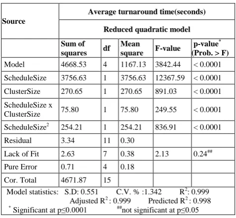
ANNOVA analysis shown in table 3 of the quadratic model for ATT reveals that the model and the model terms except ClusterSize2 term are significant at p≤0.0001. ANNOVA analysis of reduced quadratic model after ClusterSize2 term is eliminated from the model is shown in table 3. High values of coefficient of determination R2=0.999, adjusted R2 =0.999, predicted R2 =0.998 and insignificant lack of fit p-value 0.24 determine the goodness of the fit of the model to accurately predict ATT values.

ATT responses of the LJF policy are fitted to second order quadratic equation with the help of MLS based multiple regression analysis. The reduced quadratic equation in terms of unitless regression coefficients of input variables is shown in (3).

Table III. ANNOVA analysis and model statistics

Source

Average turnaround time(seconds)

Reduced quadratic model

Sum of squares df

Mean

square F-value

p-value*

(Prob. > F)

Model 4668.53 4 1167.13 3842.44 < 0.0001

ScheduleSize 3756.63 1 3756.63 12367.59 < 0.0001

ClusterSize 270.65 1 270.65 891.03 < 0.0001

ScheduleSize x

ClusterSize 75.80 1 75.80 249.55 < 0.0001

ScheduleSize2 254.21 1 254.21 836.91 < 0.0001

Residual 3.34 11 0.30

Lack of Fit 2.63 7 0.38 2.13 0.24##

Pure Error 0.71 4 0.18

Cor. Total 4671.87 15

Model statistics: S.D: 0.551 C.V. % :1.342 R2: 0.999 _{Adjusted R}2 _{: 0.999 Predicted R}2 _{: 0.998}

* _{Significant at p≤0.0001} ##_{not significant at p≤0.05}

where ScheduleSize and ClusterSize represent the coded values of input variables schedule size and cluster size respectively.

The polynomial regression equation of ATT for LJF policy in terms of actual factors is given in (4).

ATT = 27.2783 – 0.1322 SS + 0.5484 CS – 0.0156 SS x CS + 0.0036 ScheduleSize2(4).

where SS and CS represent the actual values of input variables schedule size and cluster size respectively.

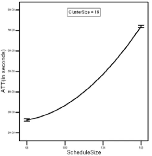
The ATT coded Eq.(3) is not only used to understand the relationship between input scheduling variables and the output response but also helps in identifying the relative importance of process variables in terms of the relative effect that they produce on the output ATT. Positive high value of regression coefficient (19.7473) of variable ScheduleSize in (3) shows that variable is mostly affecting the output and mainly responsible for producing high values of the ATT as shown in figure 5(a) and 5(b). ClusterSize has antagonistic effect on the ATT as shown by the negative value of regression coefficient (5.1042). Increase in the ClusterSize will result into decrease in the ATT values. Interaction effect also exists between Schedule size and cluster size which is shown by the term (ScheduleSize x ClusterSize) in the equation. Negative regression coefficient of the interaction term in (3) indicates that combined effect of simultaneous increase in the ScheduleSize and ClusterSize result into net negative impact on the ATT values.

Main effect plot of ScheduleSize vs. ATT in figure 5(a) and 5(b) indicates that ATT increases with the increase in the ScheduleSize. But the ATT increase is relatively smaller in figure 5(b) as compared to figure 5(a) due to relative increase in the value of ClusterSize in figure 5(b). Main effect plot of ClusterSize vs. ATT in figure 6(a) and 6(b) indicates that ATT decreases with the increase in the ClusterSize. There is not much ATT decrease in figure 6(a) as compared to figure 6(b) due to the fact that when the ScheduleSize i.e. workload on the scheduling system is small (i.e. 66) then merely increasing ClusterSize will not produce much decrease in ATT values.

Figure 5(a): Main effect plot of ScheduleSize vs. ATT at ClusterSize=16

Figure 5(b): Main effect plot of ScheduleSize vs. ATT at ClusterSize=24

Figure 5(a): Main effect plot of ClusterSize vs. ATT at ScheduleSize=66

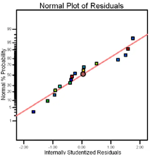
Normality assumption of the empirical model is represented by the normality plot in figure 7 which clearly shows that model residuals are distributed normally over the linear line.

Figure 6. Normal probability plot of residuals

Actual ATT values for LJF can be obtained from (4) by fitting the actual values at all the levels of WSS and CS. ATT model for LJF is validated against the additional actual experimentation results shown in table 4. Additional experi-mental values are found to be close to the predicted values.

Table IV. Validation experiments for LJF model

Exp.

No. SS CS

Predicted ATT

Exp. ATT

ANN ATT

1. 66 18 25.37 26.08 25.46

2. 134 22 39.45 39.87 39.71

3. 134 24 36.36 36.77 36.85

4. 168 20 63.91 64.23 63.52

A. ANN Predictions

Statistical data analysis software SPSS 16.0 is used to develop the MLP network model based on the experimental data provided by the DOE phase. Two inputs ScheduleSize and ClusterSize are represented by two neuron nodes in the input layer and the output layer has one neuron representing the output variable ATT. The ANN structure with two hidden neurons is chosen that gave least MSE value and better prediction of the output for both training and validation sets. The whole network information is shown in table 5.

Hyperbolic tangent activation function was used for mapping data from input to hidden layer and identity activation function was used for hidden layer to output mapping. Batch training algorithm combined with scaled conjugate gradient training optimization algorithm was used for ANN training and adjusting weights of the network respectively.

Table V. Network information

ANN layers Details

Input Layer

Input variable 1 Input variable 2

Number of Neurons a

Rescaling Method for Covariates

ScheduleSize ClusterSize 2 Adjusted Normalized

Hidden Layer

Number of Hidden Layers Number of Units in Hidden Layer 1a

Activation Function

1 2 Hyperbolic tangent

Output Layer

Dependent Variable 1 Number of Neurons

Rescaling for Scale Dependents Activation Function

Error Function

ATT 1

Standardized Identity Sum of squares error

a. Excluding the bias neuron unit

Out of the total experimental data available for ANN modeling, 66.7% was used for ANN training, 20.8% data was used for testing and rest 10.5% was used as holdout sample for validation of the network model.

Figure 8. ANN structure (2-2-1)

Training phase stops when there is no further decrease in MSE value. The trained network gave MSE value of 0.016 with regression coefficient of 0.999. The ATT predictions done by the ANN model are shown in table 2 and table 4. These ANN predictions are found to be very close to the RSM based quadratic model predictions hence ANN model validates the predictions of RSM based model. The structure of the generated ANN model is shown in figure 8 and ANN synaptic weights from input layer to hidden layer and hidden layer to output layer are shown in table 6.

Table VI. ANN synaptic weights

Input layer to hidden layer weights Hidden Layer 1

Neuron1 Neuron 2

Input Layer

(Bias) ScheduleSize ClusterSize

-0.496 0.698 -0.242

-1.001 1.136 -0.222

Hidden layer to output layer weights Output layer

Hidden Layer 1

(Bias) Neuron1 Neuron 2

IV. CONCLUSIONS

Response surface methodology (RSM) approach of DOE is used for fitting the parallel space-sharing scheduling process experimental data in the form of empirical model obtained in relation to the experimental design. The reduced quadratic empirical model for LJF policy is expressed in terms of main and interaction effects of scheduling process variables viz. schedule size and cluster size and it is found to be outstandingly statistically fit (adjusted R2=0.999) for predicting the process response ATT. Predicted values of RSM based ATT model of LJF policy are also validated against additional actual experimental results as well as ANN predictions. The benefit of two-phase modeling strategy is that first DOE oriented phase helps in understanding the mathematical relationship of input scheduling process variables with the output response whereas ANN fails to express such relationship. In second phase once the ANN model is trained and developed from experimental data passed from first phase, it offers enormous flexibility to adapt new unknown problems of the same LJF space-sharing scheduling class without redeveloping the model. Contrarily RSM based empirical model needs to be reconstructed when new design points are added to the experimental design.

V. REFERENCES

[1] R. Evard, N. Desai, J. Navarro, and D. Nurmi, “Clusters as

large-scale development facilities,” Proc.2002 IEEE International Conference on Cluster Computing (Cluster 2002), Chicago, USA, Sep. 2002.

[2] Kuzmin A. Cluster approach to high performance Computing.

Computer Modelling and New Technologies, 7, 7-15, 2003.

[3] C.T. Yang, C.C. Hung, and C.C. Soong, (2001) “Parallel

Computing on Low-Cost PC-Based SMPs Clusters,” Proc. of the 2001 International Conference on Parallel and Distributed Computing, Applications, and Techniques (PDCAT 2001),

[4] C.T. Yang, “Using a PC Cluster for High Performance

Computing and Applications”. Tunghai Science Vol. 4: 103−125, July 2002.

[5] M. Ismail, “Space-sharing job scheduling policies for parallel

computers”, Ph.D thesis, Iowa state university, Iowa, 1995.

[6] S. M.Figueira, “Optimal partitioning of nodes to

space-sharing parallel tasks”, Parallel Computing, 32(2004), 313-324.

[7] S. Iqbal, R. Gupta and Y.C. Fang, “Planning considerations

for job scheduling in HPC clusters”, reprinted from Dell Power Solutions, February 2005, pp 133-136.

[8] U.Schweigelshohn, R. Yahyapour, “Analysis of

first-come-first-serve parallel job scheduling", In SODA ’98: Proceedings of the ninth annual ACMSIAM symposium on discrete algorithms, pages 629–638, Philadelphia, PA, USA, 1998. Society for Industrial and Applied Mathematics.

[9] K. Aida, “Effect of job size characteristics on job scheduling

performance”, In Job Scheduling Strategies for Parallel Processing, Springer Verlag, Lect. Notes Computer Science vol. 1911, pp. 1--17, 2000.

[10]U. Lublin and D.G. Feitelson, "The Workload on Parallel

Supercomputers: Modeling the Characteristics of Rigid Jobs", Journal of Parallel and Distributed Computing, 63(11):1105– 1122, 2003.

[11]J. Sherwani, N. Ali, N. Lotia, Z. Hayat, and R. Buyya, “Libra:

A Computational Economy based Job Scheduling System for Clusters”, Software: Practice and Experience, vol. 34, no. 6, May 2004, pp.573-590.

[12]K. Aida, H. Kasahara, and S. Narita. "Job Scheduling Scheme

for Pure Space Sharing Among Rigid Jobs", In fourth workshop on Job Scheduling Strategies for Parallel Processing, Lecture Notes in Computer Science, vol. 1459, pages 98-121, Springer-verlag, 1998.

[13]W. F. Boyer. Efficient scheduling techniques and performance

evaluation methods for heterogeneous distributed computing systems, Ph.D thesis, University of Idaho, May 2004.

[14]L.K.Goh and B.Veeravalli, “Design and performance

evaluation of combined first-fit task allocation and migration studies in mesh multiprocessor systems”, Parallel Computing, 34(9), 508-520, 2008.

[15]A. Snavely, L. Carrington, N. Wolter, J. Labarta,R. Badia, and

A. Purkayastha, “A Framework for Application Performance Modeling and Prediction” In Supercomputing 02: Proceedings of the 2002 ACM/IEEE Conference on Supercomputing, pages 1–17, Los Alamitos, CA, 2002. IEEE Computer Society Press.

[16]N. Nissanke, A. Leulseged, and S. Chillara." Probabilistic

Performance Analysis in Multiprocessor Scheduling," J. Computing and Control Engineering, 13(4):171–179, 2002.

[17]A. Leulseged and N. Nissanke. "Probabilistic Analysis of

Multi-processor Scheduling of Tasks with Uncertain Parameters", In Proceedings of the 9th International Conference on Real-Time and Embedded Computing Systems and Applications (RTCSA 2003), LNCS 2968:103–122, Springer-Verlag, 2004.

[18]D. C. Montgomery, Design and analysis of experiments (5th

ed.). New York: Wiley & Sons, Inc. 672 pp.2009.

[19]J. Antony, Design of experiments for engineers and scientists.

Elsevier Science & Technology Books 2003.

[20]R. H. Myers, D. C. Montgomery and Anderson-Cook, C. M.,

Response Surface Methodology: Process and product optimization using designed experiments (3rd ed.).New York: John Wiley and Sons, Inc. 728 pp.2009.

[21]C. S. Yeo, R. Buyya and H. Pourreza, “Cluster Computing:

High-Performance, High-Availability and High-Throughput Processing on a Network of Computers”, vol.29 (6), Springer Science + Business Media Inc, New York, USA, 2006, pp.521-551.

[22]M. Hamdi, Y. Pan, B. Hamidzadeh and F. M. Lim, "Parallel

Computing on an Ethernet Cluster of Workstations: Opportunities and Constraints", The Journal of Supercomputing, 13, 111-132, 1999.

[23]R. Buyya, T. Cortes, and H. Jin, “Single System Image

[24]M. J. Anderson and P. J. Whitcomb, DOE Simplified: Practical Tools for Effective Experimentation, Productivity press, 2000.

[25]Design Expert Software version 8.0 user’s guide 2009.

[26]D. E. Akyol, “Application of neural networks to heuristic

scheduling algorithms”, Computers & Industrial Engineering 46(2004) 679-696.

[27]M. Salim,A.Manzoor,K.Rashid, “ A Novel ANN load

balancing technique for heterogeneous environment”, Information Technology Journal 6(7),1005-1012,2007.

[28]F.Dobslaw, “A parameter-tuning framework for

metaheuristics based on design of experiments and artificial neural networks”, World Academy of Science, Engineering and Technology 64,213-216, 2010.

[29]SPSS Software version 16.0 user’s guide 2010.

SHORTBIODATAOFTHEAUTHOR

Amit Chhabra is Assistant Professor with the department of Computer Science & Engineering, Guru Nanak Dev University, Amritsar. His research interests include modeling of parallel job scheduling algorithms, resource management systems, distributed processing and application of Design of Experiments (DOE) in various scheduling problems.

Dr. Gurvinder Singh is Associate Professor with the department of Computer Science & Engineering, Guru Nanak Dev University, Amritsar. His research interests include simulation of parallel job scheduling algorithms, genetic algorithms and network based distributed processing.

APPENDIXA WORKLOADINFORMATION

Workload Workload description: with job arrival order

Workload format (Job no. - Job name - job width - problem size)

Input parameter ScheduleSize =

Size(i))

Workload 1 No. of jobs =10

J1-Runlength Image Compression-2-303x239, J2-Matrix Vector Product.-8-3000x1, J3-Matrix Multiplication-4-256x256,J4-Matrix Multiplication-16-800x800,J5-Calculation of PI-2-100000, J6-Finding Total Prime No-4-10000,J7-Matrix Multiplication-16-800x800,J8-Matrix Multiplication-2-128x128, J9-Matrix Vector Product-8-2400x1,J10-Runlength Image Compression-4-303x239

66

Workload 2 No. of jobs =15

J1-Runlength Image Compression-2-303x239, J2-Matrix Vector Product-8-3000x1, J3-Matrix

Multiplication-4-256x256,J4-Matrix Multiplication-16-800x800,J5-Calculation of

PI-2-100000,J6-Finding Total Prime No-4-10000,J7-Matrix Multiplication-16-800x800,J8-Matrix Multiplication-2-128x128, J9-Matrix Vector Product-8-2400x1,J10-Runlength Image Compression-4-303x239,J11-Matrix Multiplication-4-256x256,J12-Matrix Vector Product-8-2000x1,J13-Finding Total Prime No-2-10000,J14-Matrix Multiplication-16-512x512,J15-Runlength Image Compression-4-303x239

100

Workload 3 No. of jobs =20

J1-Runlength Image Compression-2-303x239, J2-Matrix Vector Product-8-3000x1, J3-Matrix

Multiplication-4-256x256,J4-Matrix Multiplication-16-800x800,J5-Calculation of

PI-2-100000,J6-Finding Total Prime No-4-10000,J7-Matrix Multiplication-16-800x800,J8-Matrix Multiplication-2-128x128, J9-Matrix Vector Product-8-2400x1,J10-Runlength Image Compression-4-303x239, J11-Matrix Multiplication-4-256x256,J12-Matrix Vector Product-8-2000x1,J13-Finding Total Prime No-2-10000,J14-Matrix Multiplication-16-512x512,J15-Runlength Image Compression-4-303x239,J16-Calculation of PI-2-100000,J17-Matrix Multiplication-16-800,J18-Matrix Multiplication-4-256x256,J19-Matrix Vector Product-8-3000x1,J20-Runlength Image Compression-2-303x239

134

Workload 4 No. of jobs =25

J1-Runlength Image Compression-2-303x239, J2-Matrix Vector Product-8-3000x1, J3-Matrix Multiplication-4-256x256,J4-Matrix Multiplication-16-800x800,J5-Calculation of PI-2-100000,J6-Finding Total Prime No-4-10000,J7-Matrix Multiplication-16-800x800,J8-Matrix Multiplication-2-128x128, J9-Matrix Vector Product-8-2400x1,J10-Runlength Image Compression-4-303x239,J11-Matrix Multiplication-4-256x256,J12-Matrix Vector Product-8-2000x1,J13-Finding Total Prime No-2-10000,J14-Matrix Multiplication-16-512x512, J15-Runlength Image Compression-4-303x 239,J16-Calculation of PI-2-100000,J17-Matrix Multiplication-16-800x800,J18-Matrix Multiplication-4-256x256,J19-Matrix Vector Product-8-3000x1,J20-Runlength Image Compression-2-303x239,J21-Calculation of PI-4-1000000,J22-Matrix Multiplication-6-512x512,J23-PI-4-1000000,J22-Matrix Multiplication-8-512x512,J24-PI-4-1000000,J22-Matrix Multiplication-16-1000x1000,J25-Matrix Vector Product-2-1000x1

168