An extended abstract of this paper is published in the proceedings of the 8th International Conference on Information-Theoretic Security—ICITS 2015. This is the full version.
The Chaining Lemma and its Application
Ivan Damg˚ard∗1, Sebastian Faust†2, Pratyay Mukherjee‡1, and Daniele Venturi3 1Department of Computer Science, Aarhus University
2Security and Cryptography Laboratory, EPFL
3Department of Computer Science, Sapienza University of Rome
February 18, 2015
Abstract
We present a new information-theoretic result which we call the Chaining Lemma. It considers a so-called “chain” of random variables, defined by a source distributionX(0)with high min-entropy and a number (say,tin total) of arbitrary functions(T1, . . . , Tt)which are applied in succession to
that source to generate the chainX(0) −→T1 X(1) −→T2 X(2)· · · Tt
−→X(t). Intuitively, the Chaining
Lemma guarantees that, if the chain is not too long, then either (i) the entire chain is “highly random”, in that every variable has high min-entropy; or (ii) it is possible to find a pointj(1≤j≤t) in the
chain such that, conditioned on the end of the chain i.e. X(j) Tj+1
−→ X(j+1)· · · Tt
−→ X(t), the
preceding partX(0) T1
−→X(1)· · ·−→Tj X(j)remains highly random. We think this is an interesting information-theoretic result which is intuitive but nevertheless requires rigorous case-analysis to prove.
We believe that the above lemma will find applications in cryptography. We give an example of this, namely we show an application of the lemma to protect essentially any cryptographic scheme against memory-tampering attacks. We allow several tampering requests, the tampering functions can be arbitrary, however, they must be chosen from a bounded size set of functions that is fixed a priori.
1
Introduction
Assume that we have a uniform random distribution over some finite setX, represented by a discrete random variableX. Let us now apply an arbitrary (deterministic) functionT toXand denote the output random variable byX0 =T(X). SinceT is an arbitrary function, the variableX0can also be arbitrarily distributed. Consider now the case whereX0 is “easy to predict”, or more concretely whereX0 has “low” min-entropy. A natural question, in this case, ishow much information canX0reveal aboutX? or more formally,how much min-entropy canXhave if we condition onX0?
Intuitively, one might expect that since X0 has low entropy, it cannot tell us much aboutX, soX
should still be “close to random” and hence have high entropy. While this would be true for Shannon entropy, it turns out to be completely false for min-entropy. This may seem a bit counter-intuitive at first,
∗
Partially supported by Danish Council for Independent Research via DFF Starting Grant 10-081612.
†
Supported by the Marie Curie IEF/FP7 project GAPS, grant number: 626467.
‡
but is actually easy to see from an example: LetT be the function which maps half of the elements inX
to one “heavy” point but is injective on all the other elements. For thisT, the variableX0has very small min-entropy (namely 1) because the heavy point occurs with probability 1/2. But on the other hand,X0
reveals everything about Xhalf the time, and so the entropy ofX in fact decreases very significantly (on average) whenX0 is given. So despite having very low min-entropy,X0 =T(X)does reveal a lot aboutX.
There is, however, a more refined statement that will be true for min-entropy: LetE be the event thatXtakes one of the values that arenotmapped to the “heavy point” byT, whileE¯ is the event that
Xis mapped to the heavy point. Now, conditioned onE, bothX|EandX|0E have high min-entropy. On
the other hand, conditioned onE¯,X|E¯ will clearly have the same (high) min-entropy whether we are
givenX|0E or not
This simple observation leads to the following conjecture: there always exists an eventE such that: (i) Conditioned onE, bothXandX0have “high” min-entropy, (ii) conditioned onE¯,X0reveals “little” aboutX. In this paper, from a very high-level, we mainly focus into settling (a generalization of) this conjecture, which results in our main contribution: the information-theoretic lemma which we call the Chaining Lemma.
Main question. Towards generalizing the above setting let us rename, for notational convenience, the above symbols as follows:X(0)≡X,T1≡T andX(1)≡X0. We considert(deterministic) functions
T1, T2, . . . , Ttwhich are applied to the the variables sequentially starting fromX(0). In particular, each
Tiis applied toX(i−1)to produce a new variableX(i) = Ti(X(i−1))fori∈ [t]. We call the sequence
of variables(X(0), . . . , X(t))a “chain” which is completely defined by the “source” distributionX(0)
and the sequence of tfunctions(T1, . . . , Tt). It can be presented more vividly as follows: X(0) T1 −→
X(1)−→T2 X(2)· · · Tt
−→X(t).
We are now interested in the min-entropy ofX(1), . . . , X(t). Of course, each variableX(i)has min-entropy less than (or equal to) the preceding variableX(i−1)(as a deterministic function can not generate randomness). Assume now that we fix some threshold valueuand consider any value of min-entropy less thanuto be “low”. Assume further that the source has min-entropy much larger thanu. As a motivation, one may think of a setting where eachX(i)is used as key in some cryptographic application, where, as longX(i) has high min-entropy we are fine and the adversary will not learn something he should not. But ifX(i)has low min-entropy, things might go wrong and the adversary might learnX(i).
Now, there are two possible scenarios for the above chain: either (i) all the variables (hence the last variableX(t)) in the chain have high min-entropy; or (ii) one or more variable (obviously including the last variableX(t)) has low min-entropy. In case (i), everything is fine. But in case (ii), things might go wrong at a certain point. We now want to ask if we can at least “save” some part of the chain, i.e.,can we find a point in the chain such that if we condition on all the variables after that point, all the preceding variables (obviously including the sourceX(0)) would still have high min-entropy? This hope might be justified ift is small enough compared to the entropy ofX(0): since the entropy drops belowu after a small number of steps, there must be a point (sayj) where the entropy falls “sharply”, i.e.,X(j)has much smaller min-entropy thanX(j−1). However, as the above example shows, even if there is a large gap in min-entropy between two successive variables (X(j)andX(j−1)in this case), the succeeding one (X(j)) might actually reveal a lot about the preceding one (X(j−1)) on average. So it is not clear that we can usejas the point we are looking for. However, one could hope that a generalised version of the above conjecture might be true, namely there might exist some event, further conditioning on which, all variables would have high min-entropy, and on the other hand, conditioning on the complement,
Lemma 1 (The Chaining Lemma, informal). Let X(0) be a uniform random variable over X and
(T0, . . . , Tt) be arbitrary functions mapping X → X and defining a chain X(0) T1
−→ X(1) −→T2
X(2)· · · Tt
−→X(t). If the chain is “sufficiently short”, there exists an eventEsuch that (i) ifE happens, then all the variables(X(0), . . . , X(t)) (conditioned onE) have “high” min-entropy; otherwise (ii) if
E does not happen there is an indexjsuch that conditioning onX(j) (and also onE¯) all the previous variables namelyX(0), . . . , X(j−1)have “high” min-entropy.
Application to tamper-resilient cryptography. Although we think that the Chaining Lemma is in-teresting in its own right, in this paper we provide an application in cryptography, precisely in tamper-resilient cryptography. In tamper-tamper-resilient cryptography the main goal is to “theoretically” protect cryp-tographic schemes against so-called fault attacks which are found to be devastating (as shown by [5, 12] and many more). In this model, the adversary, in addition to standard black-box access to a primitive, is allowed to change its secret state [9, 27, 22, 31, 8], or its internals [29, 26, 18, 19], and observes the effect of such changes at the output. In this paper we restrict ourselves to the model where the adversary is not allowed to alter the computation, but only the secret state (i.e. only the memory of the device, but not the circuitry, is subject to tampering).
To illustrate such memory tampering, consider a digital signature scheme Signwith public/secret key pair (pk,sk). The tampering adversary obtains pk and can replace sk with T(sk) for arbitrary tampering functionT. Then, the adversary gets access to an oracle Sign(T(sk),·), i.e., to a signing oracle running with the tampered keyT(sk). As usual the adversary wins the game by outputting a valid forgery with respect to the original public keypk.1 In the most general setting, the adversary is allowed to ask an arbitrary polynomial number of tampering queries. However, a general impossibility result by Gennaro et al.[27] shows that the above flavour of tamper resistance is unachievable without further assumptions. To overcome this impossibility one usually relies on self-destruct (e.g., [22, 15, 1, 14, 13, 23, 24, 25, 17, 2, 3, 4, 16, 30]), or limits the power of the tampering function (e.g., [9, 33, 7, 6, 28, 35, 37, 10, 11, 30, 36]).
Recently Damg˚ard et al. [20] proposed a different approach where, instead of limiting the type of allowed modifications, one assumes an upper bound on the number of tampering queries that the adversary can ask, so that now the attacker can issue some a-priori fixed numbertofarbitrarytampering queries. As argued by [20], this limitation is more likely to capture realistic tampering attacks. They also show how to construct public key encryption and identification schemes secure against bounded leakage2and tampering (BLT) attacks.
The above model fits perfectly with the setting of the Chaining Lemma, as we consider a limited number of tampering functions(T1, . . . , Tt), for some fixed boundt, applied on a uniform (or close to
uniform) secret-stateX(0). Now recall that Lemma 1 guarantees that, for “small enough”t, the source distribution stays unpredictable in essentially “any” case. Therefore, the source can be used as a “highly unpredictable” secret-key resistingtarbitrary tampering attacks. As a basic application of the Chaining Lemma, we show in Section 4 thatanycryptographic scheme can be made secure in the BLT model. To the best of our knowledge, this is the first such general result that holds for arbitrary tampering functions and multiple tampering queries. The price we pay for this is that the tampering functions must be chosen from a bounded-size set that is fixed a priori.
Previous work by Faustet al.[25], shows how to protect generically against tampering using a new primitive callednon-malleable key-derivation. This result also works for arbitrary tampering functions, does not require that a small set of functions is fixed in advance, but works only for one-time tampering.
1
Notice thatT may be the identity function, in which case we get the standard security notion of digital signature scheme as a special case.
2
2
Preliminaries
We review the basic terminology used throughout the paper.
2.1 Notation
For n ∈ N, we write[n] := {1, . . . , n}. Given a set S, we writes ← S to denote that elementsis sampled uniformly fromS. IfAis an algorithm,y ←A(x)denotes an execution ofAwith inputxand outputy; ifAis randomized, thenyis a random variable.
We denote withkthe security parameter. A functionδ(k)is callednegligibleink(or simply neg-ligible) if it vanishes faster than the inverse of any polynomial in k. A machine A is called proba-bilistic polynomial time (PPT) if for any input x ∈ {0,1}∗ the computation of A(x) terminates in at mostpoly(|x|)steps andAis probabilistic (i.e., it uses randomness as part of its logic). Random vari-ables are usually denoted by capital letters. We sometimes abuse notation and denote a distribution and the corresponding random variable with the same capital letter, sayX. We write sup(X) for the support of X. Given an eventE, we let X|E be the conditional distribution of X conditioned on E
happening. The statistical distance of two random variablesX andY, defined over a common setS is
∆(X;Y) = 12P
s∈S|Pr [X =s]−Pr [Y =s]|. Given a random variableZ, the statistical distance of
XandY conditioned onZis defined as∆(X;Y|Z) = ∆((X, Z); (Y, Z)).
2.2 Information Theory Basics
The min-entropy of a random variableXover a setX is defined asH∞(X) :=−log maxxPr [X =x],
and measures howXcan be predicted by the best (unbounded) predictor. The conditional average min-entropy [21] ofXgiven a random variableZ(over a setZ) possibly dependent onX, is defined as
e
H∞(X|Z) :=−logEz←Z[2−H∞(X|Z=z)] =−log
X
z∈Z
Pr [Z =z]·2−H∞(X|Z=z).
We say that a distribution X over a set X of size |X | = 2n is (α, n)-good if H
∞(X) ≥ α and
Pr [X=x]≥2−nfor allx∈sup(X).
We will rely on the following basic properties (see [21, Lemma 2.2]).
Lemma 2. For all random variablesX, ZandΛover setsX,Zand{0,1}λsuch that
e
H∞(X|Z)≥α, we have that
e
H∞(X|Z,Λ)≥He∞(X|Z)−λ≥α−λ.
The above lemma can be easily extended to the case of random variablesΛwith bounded support, i.e.,He∞(X|Z,Λ)≥He∞(X|Z)−log|sup(Λ)|.
Lemma 3. For any > 0,H∞(X|Z =z)is at leastHe∞(X|Z)−log(1/) with probability at least
1−over the choice ofz.
3
The Chaining Lemma
Before presenting the statement and proof of the Chaining Lemma, we state and prove two sub-lemmas. We do not provide any intuitions at this point regarding the whole proof of the Chaining Lemma due to involvement of rigorous case-analysis. Instead, we take a modular approach presenting intuitions step-by-step for each of the sub-lemmas and finally providing an intuition of the Chaining Lemma after the proof of these sub-lemmas.
Lemma 4. For n ∈ N>1 let c be some parameter such that√n < c < n. Let X be a set of size
2n = |X |andX be a distribution overX with|sup(X)|> 2csuch that for all x ∈ sup(X)we have
Pr[X=x]≥ 21n. There exists an eventEsuch that:
(i) H∞(X|E)> c−2
√
n, and
(ii) |sup(X|E)|<|sup(X)|.
Proof. Intuitively, the lemma is proven by showing that if a distribution has sufficiently large support, then over a large subset of the support the distribution must be “almost” flat. We will describe below what it means for a distribution to be “almost flat”. We then define an eventEthat occurs whenXtakes some value in the almost flat area. Clearly,Xconditioned onEmust be “almost” uniformly distributed, and if furthermore the support ofX conditioned onE is still sufficiently large, we get thatH∞(X|E)
must be large. We proceed with the formal proof.
We introduce a parameter bwhich is a positive integer such thatc > n/b. We explain how to set the value ofblater. For ease of description we assume thatnis a multiple ofb. We start by defining what it means for an area to be flat. For some probability distributionXwe definek∈[2n/b−1]sets as follows:
• Ik:=
n
x∈sup(X) : 2knb ≤Pr[X =x]<
(k+1)b 2n
o
, fork∈[2n/b−1]and
• I2n/b :={x∈sup(X) : Pr[X=x] = 1}.
These sets characterize the (potential) flat areas in the distribution X as the probability of all values in some set Ik lies in a certain range that is bounded from below and above. Clearly, the sets Ik are
pairwise disjoint and cover the whole space between1/2n and1. Therefore, eachx ∈ sup(X) with some probabilityPr[X=x]must fall into some unique setIk.
We denote byImthe set that contains the most elements among all setsIk, and define the eventE
as the event that occurs whenx∈sup(X)falls intoIm, i.e.,Xtakes a value that falls in the largest set
Im. We now lower bound the probability thatEoccurs.
Pr[E]≥ |Im|
mb
2n (1)
≥2c−n/bm
b
2n. (2)
Inequality (1) holds as for allx∈Imwe havePr[X=x]≥ m
b
2n. (2) follows from the fact thatImmust
have size at least2c−n/b, as there are2n/bsets and there are at least2celements in the support ofX. AsH∞(X|E) =−log maxxPr[X =x|E], we can give a lower bound for the min entropy ofX|E
by upper boundingPr[X=x|E]. More precisely,
Pr[X =x|E] = Pr[X=x∧E] Pr[E]
< (m+ 1)
b/2n
2(c−n/b)mb/2n (3)
=
1 + 1
m
b
2−c+n/b
≤2b−c+n/b. (4)
Inequality (3) uses (2) and the fact thatPr[X=x∧E]< (m2+1)n b by definition ofIm. (4) follows from
Ω
E10 E001
E20 E200
E30 E300
Ω
E100 E30
E200 E300
Figure 1: Events covering the probability space in the proof of Lemma 5 and Lemma 6.
by(b+n/b)is minimum whenb=√n. Sincebis a free parameter, we fixb:= √n(note that, since
c >√n, the constraintc > n/bholds) to getH∞(X|E)> n−2
√
nas stated in part (i) of the lemma. For part (ii), it is easy to see from the definition of E that the support of the conditional prob-ability distribution X|E decreases by at least2(c−n/b) points (as these points belong to E). Clearly,
|sup(X|E)| ≤ |sup(X)| −2c−n/b <|sup(X)|as stated in the lemma.
In the following lemma we consider an arbitrary distributionX with sufficiently high min-entropy and some arbitrary functionT. We show that if the support ofY =T(X)is sufficiently large, then there exists an eventEsuch that one of the following happens:
(i) The min-entropy ofY conditioned on the eventEis high, i.e.,Y conditioned onEhas an almost flat area with large support;
(ii) IfE happens, then the average min-entropy ofXgivenY is high. Intuitively, this means thatY
conditioned onEhas small support as then it does not “reveal” too much aboutX. We formalize this statement in the lemma below.
Lemma 5. For n ∈ N>1 let c, αbe some parameters such that√n < c < α ≤ n. LetX be some set of size2n = |X |andX be an(α, n)-good distribution overX. For any functionT :X → X, let
Y =T(X)be such that|sup(Y)|>2c. There exists an eventEsuch that the following holds:
(i) H∞(Y|E)> c−2
√
n.
(ii) He∞(X|E|Y|E)≥α−c−log 1
1−Pr[E].
Proof. Intuitively, in the proof below we apply Lemma 4 iteratively to the distributionY to find flat areas inY. We “cut off” these flat areas until we have a distribution (derived fromY) which has sufficiently small support. Clearly such restricted Y cannot reveal too much information about X. To formalize this approach, we construct iteratively an eventE by combining the events Ei obtained by applying
Lemma 4 to Y. IfE happens then Y takes values that lie in a large flat area. On the other hand E
characterizes only a relatively small support, and hence giving suchY does not reveal much information (on average) aboutX. The formal proof with an explicit calculation of the parameters follows.
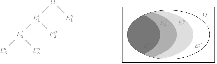
We will define the event E depending on events {Ei, Ei0, Ei00}i∈{0,...,m−1} (for some integer m) which we will specify later. These events partition the probability space as follows (cf. Figure 3):
Ei0 :=
i
^
j=0
Ej =Ei∧Ei0−1 Ei00:=Ei∧
i−1
^
j=0
Ej
We will rely on some properties of the above partition. In particular, note that for alli∈ {0, . . . , m−1}
we have
Ei0∨Ei00=Ei0−1 E
0
i∧E
00
i =∅. (6)
We start by constructing the events{Ei, Ei0, Ei00}and conditional probability distributionsY(i)that
are derived fromY by applying Lemma 4. Lemma 4 requires the following two conditions:
• |sup(Y(i))|>2c, and
• Pr[Y(i) =y]≥2−n, for ally∈sup(Y(i)).
Clearly these two conditions are satisfied byY(0) =Y, sinceY(0) is computed fromX by applying a
functionTand for allx∈sup(X)the statement assumesPr[X=x]≥2−n. Hence, Lemma 4 gives us an eventE0. We set and we defineY(1) =Y|E(0)
0. For alli
≥ 1we proceed to construct eventsEi and
conditional distributionsY(i+1)=Y|(i)
Eias long as the requirements from above are satisfied. Notice that by applying Lemma 4 to distributionY(i)we get for each eventEi:
• H∞(Y|E(i)
i)> c−2
√
n, and
• |sup(Y(i+1))|<|sup(Y(i))|.
Clearly, there are only finitely many (saym) events before we stop the iteration as the size of the support is strictly decreasing. At the stopping point we have|sup(Y(m−1))|>2cand|sup(Y(m))| ≤2c. We defineE =Wm−1
i=0 Ei =Wmi=0−1Ei00andE =
Vm−1
i=0 Ei =Em0 −1 and show in the claims below that
they satisfy conditions (i) and (ii) of the lemma. Claim 1. H∞(Y|E)> c−2
√
n.
Proof. Recall that for each0≤i≤m−1we have
Y|(Ei)
i =Y|Ei∧Ei−1...∧E0 (7) =Y|E00
i (8)
Eq. (7) follows from the definition of the conditional probability distributionY|(Ei)
i. Eq. (8) from the definition of the constructed events. From Eq. (8) and Lemma 4 we have for each0≤ i≤m−1that
H∞(Y|Ei00) > c−2
√
n. As for each0 ≤ i ≤ m−1 we have|sup(Y|E)| ≥ |sup(Y|Ei00)|we get that
H∞(Y|E)> c−2
√
n. This concludes the proof of this claim. Claim 2. He∞(X|E|Y|E)≥α−c−log 1
1−Pr[E].
Proof. We first lower boundH∞(X|E).
H∞(X|E) =−log
max
x
Pr[X=x∧E] Pr[E]
(9)
≥ −log
1
Pr[E]maxx Pr[X=x]
(10)
=H∞(X)−log
1
Pr[E] ≥α−log 1
Eq. (9) follows from the definition of min-entropy and the definition of conditional probability. Eq. (10) follows from the basic fact that for any two eventsPr[E∧E0]≤Pr[E]. Finally, we get Eq. (11) from our assumption thatH∞(X)≥α. To conclude the claim we compute:
e
H∞(X|E|Y|E)≥H∞(X|E, Y|E)−log|sup(Y|E)| (12)
=H∞(X|E)−log|sup(Y|E)| (13)
≥α−log 1
1−Pr[E]−c=α−c−log 1
1−Pr[E]. (14)
Eq. (12) follows from Lemma 2 and (13) from the fact thatY|E is computed as a function fromX|E. Inequality (14) follows from (11) and the fact that the size ofsup(Y|E)is at mostc. The latter follows from the definition of the eventE = Em0 −1 which in turn implies that |sup(Y|E)| =|sup(Y|E0m−1)|= |sup(Y|(m−1)
Em−1
)|=|sup(Y(m))| ≤2c, which concludes the proof. The above two claims finish the proof.
We now turn to state and prove the Chaining Lemma.
Lemma 6(The Chaining Lemma). Forn ∈ N>1 let α, β, t, be some parameters wheret ∈ N, 0 < α≤n,β >0,∈(0,1]andt≤ β+2α−√β
n. LetX be some set of size|X |= 2
nand letX(0)be a(α, n)
-good distribution overX. Fori ∈[t]letTi :X → X be arbitrary functions andX(i) =Ti(X(i−1)).
There exists an eventEsuch that:
(i) IfPr [E]>0, for alli∈[t],H∞(X|(Ei))≥β. (ii) IfPrE≥there exists an indexj ∈[t]such that
e
H∞(X(j −1)
|E |X
(j)
|E)≥β−log
t .
Proof. Consider the chain of random variables X(0) −→T1 X(1) −→T2 . . . −→Tt X(t). Given a pair of random variables in the chain, we refer toX(i−1)as the “source distribution” and toX(i)as the “target distribution”. The main idea is to consider different cases depending on the characteristics of the target distribution. In case the min-entropy ofX(i)is high enough to start with, we get immediately property (i) of the statement and we can immediately move to the next pair of random variables in the chain. In case the min-entropy ofX(i) is small, we further consider two different sub-cases depending on some
bound on the support of the variable. If the support ofX(i)happens to be “small”, intuitively we can condition on the target distribution since this cannot reveal much about the source; roughly this implies property (ii) of the statement. On the other hand, if the support happens to be not small enough, we are not in a position which allows us to condition onX(i).
In the latter case, we will invoke Lemma 5. Roughly this guarantees that there exists some event such that, conditioned on this event happening, the target lies in a large “flat” area and the conditional distribution has high min-entropy; this yields property (i) of the statement. If instead the event does not happen, then conditioning on the event not happening we get a “restricted” distribution with small enough support which leads again to property (ii) of the statement.
distribution and, as such, do not constrain the min-entropy further. We now proceed with the formal proof.
Similar to Lemma 5, we will define the event E depending on events {Ei, Ei0, Ei00}i∈[t] which we
will specify later. These events partition the probability space as follows (cf. Figure 3):
Ei0 :=
i
^
j=1
Ej =Ei∧E0i−1 Ei00:=Ei∧
i−1
^
j=1
Ej
=Ei∧Ei0−1. (15)
We will rely on some properties of the above partition. In particular, note that for alli∈[t]we have
Ei0∨Ei00=Ei0−1 Ei0∧Ei00=∅. (16)
For alli∈[t+ 1], define the following parameters:
si = (t−i+ 1)(β+ 2
√
n) (17)
αi−1 =β+si. (18)
Note that using the bound ontfrom the statement of the lemma, we getα≥α0; moreover, it is easy to
verify thatαi−1 > si>
√
nfor alli∈[t].
In the next claim we construct the events{Ei, Ei0, Ei00}i∈[t].
Claim 3. For alli= 0, . . . , t−1, there exist eventsEi0+1andEi00+1(as given in Eq.(16)) such that the following hold:
(*) IfPrEi0+1>0,H∞(X|(Ei+1)0 i+1)
≥αi+1.
(**) IfPrEi00+1≥0,He∞(X|(Ei)00 i+1
|X|(Ei+1)00 i+1)
≥β−log10. where0< 0 ≤1. Proof. We prove the claim by induction.
Base Case: In this case we letE0denote the whole probability space and thusPr [E0] = 1. Note that H∞(X|(0)E0) =H∞(X(0)) =α ≥α0. The rest of the proof for the base case is almost the same to that
of the inductive step except the use of the above property instead of the induction hypothesis. Therefore we only prove the induction step in detail here. The proof details for the base case are a straightforward adaptation, with some notational changes.
Induction Step: The following holds by theinduction hypothesis: (*) IfPr [Ei0]>0, thenH∞(X|(Ei)0
i)
≥αi.
(**) IfPr [Ei00]≥0 then,He∞(X
(i−1)
|Ei00 |X
(i)
|E00i)≥β−log
1
0 where0< 0 ≤1.
By construction of the events,Ei0 is partitioned into two sub-eventsE0i+1andEi00+1 (cf. Eq. 16). From the statement of the claim we observe that, since we are assumingPr
Ei0+1
>0in (*) andPr
E00i+1
≥
0 > 0in (**), in both cases we havePr [E0i]> 0. Hence, property (*) from the induction hypothesis holds: H∞(X|(Ei)0
i)
≥ αi, which we use to prove the inductive step. We will define the events Ei0+1
andEi00+1differently depending on several (complete) cases. For each of these cases we will show that property (*) and (**) hold.
Suppose first that H∞(X|(Ei+1)0 i )
≥ αi+1. In this case we define Ei0+1 to be Ei0, which implies
H∞(X|(Ei+1)0
i+1) =H∞(X (i+1)
|E0 i )
≥αi+1; as for property (**) there is nothing to prove, sincePr
E00i+1
= 0in this case.
Consider now the case that H∞(X|(Ei+1)0
i ) < αi+1. Here we consider two sub-cases, depending on the support size ofX(i+1).
1. |sup(X|(Ei+1)0 i
)| ≤ 2si+1. We define E00
i+1 = Ei0, which implies Ei0+1 = ∅ by Eq. (16). As for
property (*) there is nothing to prove, sincePr
Ei0+1
= 0. To prove property (**) we observe that ifPr
Ei00+1
≥0 >0, thenPr [Ei0]>0. Hence,
e
H∞(X|(Ei)00 i+1
|X|(Ei+1)00 i+1) =
e
H∞(X|(Ei)0 i
|X|(Ei+1)0
i ) (19)
≥H∞(X|(Ei)0 i, X
(i+1)
|E0 i )
−log(|sup(X|(Ei+1)0 i
)|) (20)
≥αi−si+1 (21)
=β+si+1−si+1 =β.
Eq. (19) follows asEi00+1 =Ei0. Eq. (20) follows from Lemma 2. Eq. (21) follows from two facts: (i)X(i+1) is a deterministic function ofX(i), which meansH∞(X|(Ei)0
i, X
(i+1)
|E0
i ) =H∞(X
(i)
|E0 i)
≥
αi (plugging-in the value from induction hypothesis), and (ii)|sup(X|(Ei+1)0 i
)| ≤2si+1.
2. |sup(X|(Ei+1)0 i
)|> 2si+1. By the induction hypothesisH
∞(X|(Ei)0 i)
≥αi; we now invoke Lemma 5
on the distributionX|(Ei+1)0
i (recall that
αi> si+1>
√
n), to obtain the eventEi+1such that: H∞(X|(Ei+1)0
i∧Ei+1)> si+1−2 √
n (22)
e
H∞(X|(Ei)0 i∧Ei+1
|X|(i+1)
Ei0∧Ei+1)> αi
−si+1−log
1 1−Pr [Ei+1]
. (23)
Note that by our definitions of the eventsEi0, Ei00(cf. Eq. (15)), we haveEi0 ∧Ei+1 =Ei0+1and
Ei0∧Ei+1=E00i+1.
To prove (*) we consider that ifPrEi0+1 >0, thenPr [Ei0]> 0andPr [Ei+1] >0. Plugging
the values ofαiandsi+1from Eq. (18) and (17) into Eq. (22), we get H∞(X|(Ei+1)0
i+1)> si+1
−2√n
= (t−i)(β+ 2√n)−2√n
=β+ (t−i−1)(β+ 2√n) =β+si+2=αi+1,
Similarly, to prove (**), we consider that ifPrEi00+1 ≥ 0, thenPr [Ei0] ≥ 0 > 0 and also
PrEi+1
≥0. Using Eq. (23), we obtain:
e
H∞(X|(Ei)00 i+1
|X|(Ei+1)00 i+1
)> αi−si+1−log
1
Pr
Ei+1
=β−log 1
Pr
Ei+1
≥β−log 1
This concludes the proof of the claim.
We define the eventE to beE =E0t = Vt
i=1Ei =
Vt
i=1E
0
i. It is easy to verify that this implies
E =Wt
i=1Ei00. We distinguish two cases:
• IfPr [E]>0, by definition ofEwe get thatPr [Ei0]>0for alli∈[t]. In particular,Pr [Et0]>0. Hence,H∞(X|(Et)) =H∞(X|(Et)0
t)≥αt=β, where the last inequality follows from property (*) of the above Claim, usingi=t−1. Also, we observe that for alli∈[t],H∞(X|(Ei−1))≥H∞(X|(Ei)). This proves property (i) of the lemma.
• IfPr
E
≥, then we get
Pr
" t _
i=1
Ei00
#
≥. (24)
t
X
i=1
Pr
Ei00
≥. (25)
Eq. (24) follows from the definition ofE and Eq. (25) follows applying union bound. Clearly, from Eq. (25), there must exists somejsuch thatPrhEj00i≥/t.
Hence, puttingi=j−1and0 =/tin property (**) of the above Claim, we get:
e
H∞(X|(Ej−001) j
|X|(Ej)00 j)
≥β−logt
.
From the definition ofE,Ej00impliesEand hence property (ii) of the lemma follows.
4
Application to Tamper-Resilient Cryptography
We show thatanycryptographic primitive where the secret key can be chosen as a uniformly random string can be made secure in the BLT model of [20] by a simple and efficient transformation. Our result therefore covers pseudorandom functions, block ciphers, and many encryption and signature schemes. However, the result holds in a restricted model of tampering: the adversary first selects an arbitrary set of tampering functions of bounded size and, as he interacts with the scheme, he must choose every tampering function from the set that was specified initially. We call this thesemi-adaptiveBLT model. Our result holds only when the set of functions is “small enough”.3
The basic intuition behind the construction using the Chaining Lemma is easy to explain. We use a random stringX0as secret key, and a universal hash functionhas public (and tamper proof) parameter.
The construction then computesK0=h(X0), and usesK0as secret key for the original primitive. The
intuitive reason why one might hope this would work is as follows: each tampering query changes the key, so we get a chain of keysX0, X1, . . . , XtwhereXi =Ti(Xi−1)for some tampering functionTi.
Recall that the chaining lemma guarantees that for such a chain, there exists an eventE such that: (i) whenE takes place then allXihave high min-entropy, and, by a suitable choice ofh, all the hash values
K0 = h(X0), K1 = h(X1), . . . , Kt = h(Xt) are statistically close to uniformly and independently
3In particular, the adversary can choose a “short enough” sequence of tampering functions, from a set containing
chosen keys; (ii) whenE does not happen, for some indexj∈[t]we are able to reveal the value ofXj
to the adversary as theXi’s withi < jstill have high entropy, and hence hash to independent values. On
the other hand theXi’s withi≥ jare a deterministic function ofXj and hence the tampering queries
corresponding to any subsequent key can be simulated easily.
Due to its generality the above result suffers from two limitations. First, as already mentioned above, the tampering has to satisfy a somewhat limited form of adaptivity. Second, the number of tampering queries one can tolerate is upper bounded by the lengthnof the secret key. While this is true in general for schemes without key update, for our general result the limitation is rather strong. More concretely, with appropriately chosen parameters our transformation yields schemes that can tolerate up toO(√3n)
tampering queries.
Comparison with Faustet al. [25]. Very recently, Faustet al. [25] introduced the concept of non-malleable key derivation which is similar in spirit to our application of the Chaining Lemma. Intuitively a function h is a non-malleable key derivation function if h(X) is close to uniform even given the output ofh applied to a related inputT(X), as long as T(X) 6= X. They show that a randomt-wise independent hash function already meets this property, and moreover that such a function can be used to protect arbitrary cryptographic schemes (with a uniform key) against “one-time” tampering attacks (i.e., the adversary is allowed a single tampering query) albeit against a much bigger class of functions.4
We stress that the novelty of our result is in discovering the Chaining Lemma rather than this appli-cation, which can be instead thought of as a new technique, fundamentally different from that of [25], to achieve security in the BLT model. We believe that the Chaining Lemma is interesting in its own right, and might find more applications in cryptography in the future.
Notation for this section. In this sectionn=poly(k)denotes the length of the key unless explicitly mentioned otherwise, wherekis the security parameter. Given some eventE we writeHe∞(X|Y1, Y2,
. . . , E)to denote that every random variable is conditioned on the eventE.
Organization. We put forward a notion of semi-adaptive BLT security for general primitives in Sec-tion 4.1. In SecSec-tion 4.2, we describe our transformaSec-tion based on universal hashing and state its security (see Theorem 1). Section 4.3 contains a high-level overview of the proof of Theorem 1; a formal proof appears in Section 4.4 and 4.5. Finally, in Section 4.6 we discuss a few extensions.
4.1 Abstract Security Games with Tampering
We start by defining a general structure of abstract security games for cryptographic schemesCS. Most standard security notions such as IND-CPA or pseudorandomness of PRFs follow the structure given below, and we will later give concrete instantiations of our abstract definition. We then show how to extend such games to the BLT setting. Consider some cryptographic scheme CS with associated key generation algorithm KeyGen. KeyGen outputs a secret key X, and in some cases some public parameterspp. We will grant the adversary access to an oracleO(pp, X,·). The definition of the oracle depends on the actual security definition. For instance, it can be a signing oracle or an oracle that gives access to the outputs of a PRF with keyK. To simplify notation, we will assume that such oracles can be multi-functional. That is, if we want to model CCA security of a symmetric encryption scheme,O
offers interfaces for both encryption and decryption queries.
Definition 1(Abstract security game). Let k ∈ Nbe the security parameter and let CS be a crypto-graphic scheme with key generation algorithmKeyGen. LetO(X,pp,·),C(X,pp,·)be some oracles,
4
whereC(X,pp,·)is the challenge oracle that outputs at the end a bitb. We assume in the following that both oracles share state. An abstract security gameGameCSC,O,A(k)consists of 3 phases given below.
1. Setup:Run the key generation(X,pp)←KeyGen(1k). The public parametersppare given toA. 2. Query phase:The adversary gets access to the oracleO(X,pp,·)and is allowed to query them in
any order.
3. Challenge phase:The adversary looses access to all oracles and interacts with the challenge oracle C(X,pp,·)that at the end outputs a bitb.bis returned by the game, whereb= 1indicates thatA won the game.
We define the security of a cryptographic scheme according to the above definition depending on whether it is an unpredictability or indistinguishability type game.
• Forunpredictabilitysecurity games we say that a scheme isδ(k)-secure if for any PPT adversary Athe advantage ofAis
Pr[GameCSC,O,A(1k) = 1]≤δ(k).
• Forindistinguishabilitygames we say that a scheme isδ(k)-secure if for any PPT adversaryAthe advantage ofAis
Pr[GameCSC,O,A(1k) = 1]−1/2≤δ(k).
For indistinguishability games, we assume wlog. that the challenger C internally keeps a bitb andA submits as its last message to C a bit b0. If b = b0 then the challenger returns 1; otherwise 0. In the following, we will usually omit the parameter δ(k)and just say that a scheme is secure if δ(k) is negligible ink.
We now extend the above definition to the BLT setting. We will give the extension specifically for the case of a semi-adaptive choice of tampering functions. Notice that BLT security can also be defined for a fully adaptive choice, but our general construction from this section does not achieve this stronger notion. We emphasize, however, that for some specific schemes fully adaptive BLT security can be achieved for free (as shown in [20]). We start by providing some intuitive description ofsemi-adaptive BLT security.
In contrast to Definition 1, in the BLT setting the adversaryAcan learnλbits about the key in the setup phase. More importantly, after the query phase he may decide on a particular choice of tampering functionsT ∈ T and gets access to the tampered oracles. Finally, in the challenge phase, he looses access to all oracles (including the tampered oracles) and plays the standard security game against the challenger C(X,pp,·). As in Definition 1 the challenge oracle outputs a bit indicating whether the adversary won or lost the BLT security game.
Definition 2 (Abstract BLT security game). Let λ, t, v be functions in the security parameter k ∈
N and let CS be a cryptographic scheme with key generation algorithm KeyGen. Let O(X,pp,·), C(X,pp,·)be some oracles, whereC(X,pp,·)is the challenge oracle that outputs at the end either0
or 1. We assume in the following that all these oracles share state. An abstract BLT-security game BLTCSC,O,A(k, t, λ, v)consists of 4 phases given below.
1. Setup: Run(X,pp) ← KeyGen(1k)and obtain fromAa description of a leakage function L :
X → {0,1}λ and a set of tolerated tampering functionsT ={(T
1, . . . , Tt)|Ti : X → X }with
2. Query phase:The adversary gets access to the oracleO(X,pp,·)and is allowed to query them in any order.
3. Tampering phase:The adversary decides on a choice of tampering functionsT = (T1, . . . , Tt)∈
T and gets access to the tampered oracles. That is, he can query (in any order) the tampered oraclesO(T1(X0),pp,·), . . .O(Tt(Xt−1),pp,·), whereX0 =XandXi =Ti(Xi−1).
4. Challenge phase:The adversary looses access to all oracles and interacts with the challenge oracle C(pp, X,·)that eventually outputs a bitb. bis returned by the game and indicates ifAwon the game.
We define BLT security for unpredictability or indistinguishability type games analogous to standard security where the adversary now runs in the BLT game as given by Definition 2.
Definition 3(Semi-adaptive BLT security ofCS). We say that a cryptographic schemeCS is(λ, t, v) -BLT-securein the semi-adaptive BLT model if for all PPT adversariesAwe have
Pr[BLTCSC,O,A(k, t, λ, v) = 1]≤negl(k).
Here,|T |=vand each element ofT is a tuple(T1, . . . , Tt)of tampering functions.
Some remarks are in order to explain the relation between the standard game GameCSC,O,A(k) and
the BLT gameBLTCSC,O,A(k, t, λ, v). Consider for instance the standard security notion of existential
un-forgeability of digital signature scheme. Our abstract security game from Definition 1 clearly covers this security notion whenO(pp, K,·)is the signing oracle and the challenge oracle returns1if the adversary submits a valid forgery toC during the challenge phase. Another example is the indistinguishability based security notion of PRFs. Here,O is the oracle that returns outputs of the PRF on inputs of the adversary’s choice, while the challenge oracle returns either the output of the PRF or the output of a ran-dom function. Notice that in this case the challenge oracle returns⊥for inputs that have been already queried to oracleO. As in the standard definition for PRFs the adversary wins the game when he can correctly tell apart random or real queries.
The BLT security game extends these abstract security games by giving the adversary additional access to tampered oracles. That is, for all an oracle O that the adversary can access in the standard security game, he now gets access to a “tampered copy” of this oracle. More precisely, for any oracleO
from the standard security game and for any set of tampering functions(T1, . . . , Tt)the adversary gets
now additionally access to the oraclesO(pp, Ti(Xi−1),·). 4.2 A General Transformation
We now describe a general transformation to leverage security of a cryptographic schemeCS (as per Definition 1) to semi-adaptive BLT security (as per Definition 3). The transformation is based on a familyH = {hS : X → Y} of(2t+ 1)-wise independent hash functions. Recall thatH is called
t-wise independent if for any sequence of distinct elementsX(1), . . . , X(t) ∈ X the random variables
hS(X(1)), . . . , hS(X(t))are uniform, wherehS ← H.5
The transformation. Consider a cryptographic schemeCS with a key generation algorithmKeyGen outputting a secret keyXand public parameterspp. In the following we consider schemes that have a BLT admissible key generation algorithm. That is, (1) the secret keyXis sampled uniformly at random from the key spaceX, and (2) given the secret keyX, there exists an efficient algorithmKeyGen0(X)
5
that takes as inputX and outputs corresponding public parameterspp. Furthermore, let CSbe some cryptographic algorithm that uses the secret keyX, the public parameterspp and some inputM and outputsZ ←CS(pp, K, M). For instance,CS may be a block cipher andCSthe associated encryption algorithm withM being the message andZ the corresponding ciphertext. We transform CS into CS0
as follows. Let H = {hS : X → Y}S∈S be a family of 2(t+ 1)-wise independent hash functions. At setup we sample a key for the hash function S and X ← X uniformly at random and compute
K = hS(X). We then runKeyGen0(K) to sample the corresponding public parameters pp, where
KeyGenis the underlying key generation ofCS. LetXbe the secret key ofCS0andpp0 = (pp, S)the corresponding public parameters. To compute the cryptographic algorithmCS0on some inputM, we run
Z ←CS(pp, hS(X), M), i.e., we map the keyXforCS0to the keyKfor the underlying cryptoscheme
CS by applying the hash function.
The theorem below states that the above transformation is BLT-secure in the semi-adaptive BLT model wheneverCS is secure in the standard sense (cf. Definition 1 and its key generation algorithm is BLT admissible.
Theorem 1. IfCSis secure andH={hS :X → Y}S∈S is a family of2(t+ 1)-wise independent hash functions with|X |= 2nand|Y| = 2`, then we have thatCS0 is(λ, t, δ, v)-secure in the semi-adaptive BLT model, where
λ=O(√3
n) t=O(√3
n) δ≤negl(k) v=O(nd) `=O(√4
n),
for some constantd >0.
Concretely, we can think ofCS being a PRF (or a signature scheme) with security in the standard sense, i.e., the adversary has negligible advantage when playing against the underlying challenger. The Theorem 1 says that, for sufficiently largen, the transformed PRFCS0achieves semi-adaptive BLT se-curity against adversaries tamperingO(√3n)times and leakingO(√3n)bits from the original key. Notice
that the hash function compresses then-bit input toO(√4n)bits and the set of admissible (sequences of)
tampering functions has sizeO(nd)for some constantd > 0. Notice that if the underlying primitive is super-polynomial secure than we can increase the size of admissible tampering functions. In the extreme case when the underlying primitive has exponential security, the size of T may be sub-exponentially large.
We emphasize that we can obtain stronger leakage resilience as we inherit the security properties from the underlying cryptoschemeCS. Hence, ifCS is secure against adaptive leakage attacks from the keyK, then alsoCS0 is secure against adaptive leakage attacks from the keyhS(X)used by the actual
cryptographic scheme.
4.3 Outline of the Proof
We explain the intuition and the main ideas behind the proof of Theorem 1. The proof is by reduction: Given an adversaryAwith non-negligible advantage in the semi-adaptive BLT game forCS0(cf. Defi-nition 3), we build an adversaryBagainst standard security ofCS(cf. Definition 1). The main difficulty is thatBhas only access to the standard oracleO(pp, K), so it is not a priori clear howBcan answer A’s tampering queries and simulate the tampered oracles.
The idea is to letBsample the initial keyX(0)independently of the target keyK (which is anyway
not known toB) and compute the keysX(1), . . . , X(t)as specified by the tampering functionsTiin order
to simulate the tampered view ofA, i.e., the oraclesO(pp0, Ti(X(i−1))). To give a first hint why this may
indeed be a good strategy, consider the simple case where all tampered keys have high min-entropy (say higher than some thresholdβ). In this case, we can rely on a property of2(t+1)-wise independent hash-ing, namely for a uniformly sampled hash functionhSthe tuple(hS(X(0)), hS(X(1)), . . . , hS(X(t)))is
Lemma 7. Let(X1, X2, . . . , Xt) ∈ Xtbet(possibly dependent) random variables such that we have
H∞(Xi)≥βand(X1, . . . , Xt)are pairwise different. LetH={hS:X → Y}be a family of2t-wise
independent hash functions, with|Y|= 2`. Then for randomhS ← Hwe have that
∆((hS, hS(X1), hS(X2), . . . , hS(Xt)); (hS, UY, . . . , UY | {z }
ttimes
))≤ t 2·2
(t·`−β)/2.
Of course, in our general tampering model nothing guarantees that all keys have high min-entropy, and hence we cannot immediately apply Lemma 7. At this point, a careful reader may object that at the end this does not matter too much: if the compression of the hash function is high enough (as it is the case for our choice of` ≈ √4nin Theorem 1) the hashed keys are short anyway, and thus the entropy
ofX(0) given the hash of the tampered keys remains high. At this point it looks tempting to apply the
leftover hash lemma, and argue thathS(X(0)) is statistically close to uniform even given the hashed
tampered keys. The leftover hash lemma, however, requires that the keyS can be sampled uniformly and independently from the distribution of X(0). Unfortunately, the conditional distribution of X(0)
(given the tampered hashed keys) may now depend onS, and we cannot apply the leftover hash lemma directly.
At this point we use the Chaining Lemma. We restate the Chaining Lemma 6 below for reader’s convenience.
Lemma 6. Forn∈N>1letα, β, t, be some parameters wheret ∈N,0 < α≤n,β >0,∈(0,1]
andt≤ β+2α−√β
n. LetX be some set of size|X |= 2
nand letX(0)be a(α, n)-good distribution overX.
Fori∈[t]letTi :X → X be arbitrary functions andX(i)=Ti(X(i−1)). There exists an eventEsuch
that:
(i) IfPr [E]>0, for alli∈[t],H∞(X|(Ei))≥β. (ii) IfPrE≥there exists an indexj ∈[t]such that
e
H∞(X|(Ej−1)|X|(Ej))≥β−log
t .
Instead of the real experiment we can now turn to a mental experiment where at some point in the chain we reveal an entire sourceX(i). By the Chaining Lemma 6 we are guaranteed thatX(0), X(1), . . . , X(i−1)individually all have high min-entropy even givenX(i), which allows us to apply Lemma 7
and conclude that hS(X(0)), . . . , hS(X(i−1)) are jointly close to uniform. Notice that in the mental
experiment clearly the remaining sourcesX(0), X(1), . . . , X(i−1)remain independent fromSeven given
X(i). At this point we are almost done except for two technical difficulties: (1) the Lemma 7 requires that
allX(j)(forj < i) are pairwise distinct, and (2) the adversary picks its tampering choiceadaptivelyfrom a fixed setT after seeing the key for the hash functionSand after interacting with the original challenger (the so-called semi-adaptive model). We solve the first by changing the above mental experiment and eliminate all sources that appear multiple times in the source chain. We then show that given a short advice we can re-sample the completeX(0), . . . , X(t)from the reduced chain. To complete the proof, we address the semi-adaptivity mentioned in (2) by a counting argument as the size of the set of potential tampering queriesT is not too big (polynomial in the security parameter).
We conclude the above outline by defining two experiments that describe how the keysX(0), X(1) , . . . , X(t) are sampled in the real game and in the simulation. Fort, λ ∈ Nand any set of functions
T1, . . . , Tt : X → X, L : X → {0,1}λ consider the two experiments as given in Figure 2. In the
ExperimentRealvs.Sim
1. ExperimentReal(X,T, L): LetX(0) be a random variable with distributionX andhS ← Ha uniformly
sampled hash function. For a sequence of functionsT1, . . . , Tt∈ T letX(i)=Ti(X(i−1))and output:
Real:= (D0, . . . , Dt+2) =
hS(X(0)), . . . , hS(X(t)), L(X(0)), S
.
2. ExperimentSim(X,T, L): Let X(0) be a random variable with distributionX andh
S ← Ha uniformly
sampled hash function. For a sequence of functionsT1, . . . , Tt ∈ T letX(i) = Ti(X(i−1)), and proceed as
follows:
SampleD0←UY.
Fori∈[t]compute:
IfX(i)6=X(0)thenDi=hS(X(i))
ElseDi=D0
OutputSim= (D0, . . . , Dt, L(X(0)), S).
Figure 2: ExperimentRealdenotes the real tampering experiment andSimour simulation.
Lemma 8. Denote withk∈Nthe security parameter and letn, t, q, v, λ, , `, αbe functions inksuch
thatλ, t < α ≤nand ∈(0,1/2). LetH ={hS :X → Y}be a family ofq-wise independent hash
functions andT ={Ti :X → X }, such that|T |= 2v. Let|X | = 2n,|Y| = 2`, andXbe an(α, n)
-good distribution overX. For all sequences of functions(T1, . . . , Tt)∈ T, and for allL:X → {0,1}λ
as specified in Figure 2:
∆(Real;Sim)≤2t(v+`)+2 q 4t22c−t`
2qt
+ 6,
wherec:=β−2 logt/−λ−2tlog(t)andβ := α−2t
√
n t+1 .
Some comments are in order to explain the mechanics of the parameters defining the statistical distance between RealandSimin Lemma 8. To obtain a negligible quantity (as we will need for the proof of Theorem 1 in Section 4.4), the valuecmust be chosen to be sufficiently larger than the value
(t+ 1)·`; this shows a clear trade-off between the value oftand the value of`. We instantiate Lemma 8 with concrete values in the following corollary. It shows a setting where we try to maximize the number of tampering queries we can tolerate by using a very high compression factor.
Corollary 1. For sufficiently largen, if we set` = O(√4n),λ = O(√3n),α = n−O(√3n) and = exp(−Θ(√3n))in Lemma 8 we gett=O(√3n)for which the distance∆(Real;Sim)≤exp(−Ω(√3n)).
4.4 Proof of Theorem 1
We now turn to the proof of Theorem 1.
Proof of Theorem 1. Suppose there exists an adversaryAand a polynomialp(.)such thatAbreaks the
(λ, t, v)semi-adaptive BLT security ofCS0with advantage at least1/p(k)for infinitely manyk. Then, we construct an adversaryBthat breaks the security ofCS according to the challenge oracleC(pp, K)
1. Setup phase:In the first stepBreceives a leakage functionL:X → {0,1}λand a set of tolerated
tampering functionsT fromA. It also receives the public parametersppfrom its own target game. Bchooses uniformly at random an indexj∗ ∈[v]. Recall thatv=|T |=O(nd)for some constant
d.
2. Bsamples a random keySfor the hash function and uniformly at random an initial keyX(0)from
X. It forwardsL(X(0))andpp0= (pp, S)as the public parameters toA.
3. Buses its underlying target oracleO(pp, K)for the cryptoschemeCS to simulateA’s interaction with the original (un-tampered) key in the query phase.
4. Breceives a tuple of tampering functions Vj = (T1, . . . , Tt) ∈ T from A. Ifj 6= j∗ then we
proceed as follows:
(a) IfBruns an unpredictability game, then it aborts.
(b) IfBruns an indistinguishability game, then it samples a random bitband submitsbas its last message to its challenge oracleC.
5. BcomputesX(i)=Ti(X(i−1))and simulates interactions with the oracles as follows:
(a) For alli ≥ 1 withX(i) 6= X(0), it usesX(i) to simulateA’s interaction with the oracles
O(pp0, hS(X(i)))in the tampering phase. AsX(i)is known toBthis can be done efficiently.
(b) For alli≥0withX(i)=X(0), it uses its target oracle to simulateA’s view. Notice that this includes the case whenAinteracts with the scheme running on the original keyX(0). We argue that whenAwins the tampering game with advantage at least1/p(k), thenBwins the under-lying game against challengerCwith advantage1/p0(k). To this end, we first show that conditioned on
j = j∗ the view of the adversary in the simulation and the adversary’s view in the real experiment are statistically close. Ifj =j∗the simulation above is identically distributed to the simulation given inSim from Figure 2. This follows from the following observations:
1. In the simulationAis committed to the tampering option j∗ beforehe starts to interact with the challenge oracles as otherwise B will abort the simulation. Notice that this commitment is in particular before seeing the hash keyS, and the view with the original key. Hence,B’s simulation corresponds to the non-adaptive case as given inSim.
2. Buses its own challenge oracle running with a uniform key to simulateA’s un-tampered view. This is exactly as in the simulationSimfrom Figure 2, where we replace the first output of the hash function with a uniformly and independently sampled value (independently ofSand the first input to the hash function).
3. B simulates the tampering queries by using an initial input X(0) for the hash function that is chosen independently from the un-tampered view. That is exactly what happens inSim.
The above concludes that the simulation ofBand the simulation given inSimare identical ifj=j∗. By Lemma 8 and Corollary 1 we get for the choice of parameters given in the theorem’s statement (notice that this choice corresponds to the parameters of Corollary 1) that forj=j∗
∆(BLTCSC,O0,A(k, t, λ, v);BLT
CS0
C,O,A(k, t, λ, v))≤exp(−Ω( 3
p
(n)), (26)
whereBLTCS 0
C,O,A(k, t, λ, v)is the game whereAruns in the experiment as defined byB. To complete the
1. Unpredictability security notion:For unpredictability gamesBaborts in Step 4 ifj 6=j∗. Hence, we get:
Pr[GameCSC,O,B(1k) = 1] = Pr[GameCSC,O,B(1k) = 1|j=j∗] Pr[j=j∗] + Pr[GameCSC,O,B(1k) = 1|j6=j
∗
] Pr[j 6=j∗] ≥Pr[GameCSC,O,B(1k) = 1|j=j∗] Pr[j=j∗]
≥Pr[BLTCSC,O0,A(k, t, λ, v) = 1]−exp(−Ω(√3n)1
v (27) > 1
p0(k). (28)
(27) follows from Eq. (26) and the fact that conditioned onj=j∗Bwins gameGameCSC,O,Bwhen AwinsBLTCSC,O0,A(k, t, λ, v). Finally, (28) holds becausev=O(nd)(for some constantd) and by assumptionPr[BLTCSC,O0,A(k, t, λ, v) = 1]≥1/p(k). Clearly, (28) yields a contradiction.
2. Indistinguishability security notion: For indistinguishability gamesBaborts and sends a random bitbto the challenger. As above we need to lower bound the advantage ofBwhen playing against the challenge oracleC.
Pr[GameCSC,O,B(1k) = 1]−1
2 = Pr[Game
CS
C,O,B(1k) = 1|j=j∗] Pr[j=j∗] + Pr[GameCSC,O,B(1k) = 1|j 6=j∗] Pr[j6=j∗]−
1 2
≥Pr[GameCSC,O,B(1k) = 1|j=j∗] Pr[j=j∗] +Pr[j6=j
∗]
2 −
1 2
(29)
≥
Pr[BLTCSC,O0,A(k, t, v, λ) = 1]−exp(−Ω(√3n))
v +
v−1
2v −
1 2
(30)
> 1
p0(k). (31)
(29) holds becausePr[GameCSC,O,B(1k) = 1|j 6=j∗] = 1/2. (30) follows from Eq. (26) and the fact that conditioned onj =j∗ Bwins its game whenAwins its BLT game. Finally, (31) holds becausev =O(nd)(for some constantd) andPr[BLTCCS,O0,A(k, t, v, λ) = 1]≥1/2 + 1/p(k)for
some polynomialp(.).
The above yields a contradiction as for both game types the adversaryBhas a non-negligible advan-tage against the underlying challengerC. Hence, we get
Pr[BLTCSC,O0,A(k, t, v, λ) = 1]≤negl(k)
as claimed in the theorem. This concludes the proof.
4.5 Proof of Lemma 8
1. Let X(0) be distributed according toX and compute X(i) = Ti(X(i−1)) (this is exactly as in
Real).
2. For alli∈[t]outputhS(X(i))if for allj < iwe haveX(i)6=X(j). Denote these outputs byD1.
We also output(L(X(0)), S).
The adviceZ (depending on X(0) and the functions T1, . . . , Tt) describes where the values fromD1
appear inReal. An easy way to describe such an adviceZrequirest2/2bits. A more thorough analysis shows that one can encode the information necessary to map from D1 toReal by 2tlog(t) bits.6 In the following we denote the mapping algorithm that maps(D1, Z)toRealasSamp(D1, Z). Clearly, Samp(D1, Z)andRealare identically distributed and all values inD1are distinct. For ease of notation we will reuse the parametertto denote the number of elements inD1.
Claim 4. Letβ= α−2t
√
n
t+1 . There exists ani∈[t]and an eventGood such thatPr[Good]≥1−and
e
H∞(X(i)|X(i+1), L(X(0)), S, Z,Good)≥β−logt/−λ−2tlog(t). (32) In the aboveX(t+1)denotes a random variable that is chosen uniformly and independently fromX.
Proof. Recall that by puttingGood in the condition of (32) we denote that all random variables are conditioned on the fact that Good happens. We prove this statement by relying on Lemma 6 which shows that eachX(i)has average min-entropy at leastβ−logt/. Lemma 6 puts a constraint onβ, i.e.,
β ≤ α−2t
√
n
t+1 . Clearly, our choice ofβ satisfies the above constraint. AsX(0) is(α, n)-good, we can
now apply Lemma 6:
1. IfPr [E]>0, for alli∈[t]:H∞(X|(Ei))≥β,
2. IfPr[E]≥then there existsi∈[t]such that :He∞(X|(Ei−1)|X|(Ei))≥β−logt.
Consider now the setting whenPr [E]>0. Hence we know by Step (1) from above that for alli∈[t]:
H∞(X|(Ei)) ≥β, and in particularH∞(X|(Et)) ≥ β. AsX(t+1)is uniformly and independently chosen from all other variables, we get in this case that
e
H∞(X|(Et)|X|(Et+1))≥β≥β−logt/. (33) Again ifPr[E]≥then by Step (2) from above there exists ani∈[t]such that
e
H∞(X|(Ei−1)|X|(Ei))≥β−logt/. (34) We defineGood as follows:Good =EifPr[E]< andGood = ΩifPr[E]≥whereΩdenotes the whole probability space. We can bound the probability of the eventGood considering two cases:
• WhenPrE≥, thenPr [Good] = 1.
• WhenPrE< then,Pr [Good] = Pr [E]>1−. So clearlyPr [Good]>1−.
We conclude that there must exist ani∈[t]such that e
H∞(X(i)|X(i+1), L(X(0)), S, Z,Good)≥He∞(X(i)|X(i+1), S,Good)−λ−2tlog(t) (35)
=He∞(X(i)|X(i+1),Good)−λ−2tlog(t) (36)
≥β−logt/−λ−2tlog(t). (37)
6This can be done by first describing for each element inD1how often it appears inRealand then by defining a mapping
Eq. (35) follows from the chain rule for conditional average min entropy (cf. Lemma 2). Eq. (36) holds becauseS is chosen uniformly and independently from all other variables. Finally, as eitherE orE
must happen and we condition onGood, we get from Eq. (33) and Eq. (34) that Eq. (37) holds. This concludes the proof of the claim.
By using the union bound and Lemma 2, we can now restate Claim 4 in terms of min-entropy and condition all random variables on eventGood happening. Thus we get that there exists ani∈[t]such that with probability at least1−2the following holds:
H∞(X(i)|(X(i+1), L(X(0)), S, Z) =r)≥β−2 logt/−λ−2tlog(t).
Recall thatX(i)can be computed as a (deterministic) function fromX(j)wherej < i. Hence, the above holds for allX(j)wherej ≤i, i.e.,
H∞(X(j)|(X(i+1), L(X(0)), S, Z) =r)≥β−2 logt/−λ−2tlog(t) =:c.
As with probability at least1−2allX(j)individually have min-entropycand by assumption allX(j)
are distinct, we can apply Lemma 7:
∆((D1, Z); (
i+1times
z }| {
UY, . . . , UY, X(i+1), L(X(0)), S
| {z }
D2
, Z))≤2t(v+`)+1
q
4t22c−t`
2qt
+ 3=:0.
AsSampis a deterministic algorithm, the above implies:
∆(Samp(D1, Z);Samp(D2, Z))≤0.
Notice that inSamp(D2, Z)the firsti+ 1values are now sampled uniformly and independently from
UY. Consider now a distributionD3 where only the first element is replaced byUY and the followingi elements are computed correctly as the output of the hash functionhS. By a standard argument, we get
∆(Samp(D1, Z);Samp(D3, Z))≤20.
To conclude the proof notice thatRealandSimare identically distributed except for the effect that the first element has on the two distributions.7Hence,Samp(D3, Z)andSimare identically distributed. As moreoverSamp(D1, Z)andRealare identically distributed this concludes the proof.
4.6 Extensions
We discuss some extensions of the result presented in this section.
Beyond semi-adaptivity. Notice that sinceT is a set of tuples of functions, Definition 3 clearly implies non-adaptive security where the adversary commits to a single chain of tampering functions(T1, . . . , Tt).
We further notice that we can obtain a stronger form of semi-adaptivity by paying a higher price in the security loss. In this model, after committing to a set of functions T = {Ti : X → X } (in
Step 1 of Definition 2), the adversary can adaptively choose individual functions fromT (in Step 3 of Definition 2). The loss in security however increases by a factorvt(instead of justvas in Theorem 1).
Finally, observe that we can replace the2(t+ 1)-wise independent hash function with any cryptographic hash function and model it in the security proof of Theorem 1 as a random oracle. As long as the tampering function cannot query the random oracle, the tampering choice may now be fully adaptively.
7
Notice also that the random oracle allows us to improve some of the parameters from the theorem—in particular, the compression rate`.
It is an interesting question if also for general primitives stronger adaptivity security notions in the BLT model can be obtained. The following simple example shows, however, that this question may be hard—at least in its most general form.
Example 1. Consider a PRF ψ(K, M) that is a function of a d-key K and input M and is secure in the standard sense (without tampering or leakage). We also assume that the function can be bro-ken if one learns a constant fraction of the key bits. We turn this into a new scheme with a public parameter x1, . . . , xdchosen from a large finite field of characteristic 2. The secret key is now a
ran-dom polynomial f of degree at mostd−1. To evaluate the function on input M, we first compute
K = (lsb(f(x1)), . . . ,lsb(f(xd)))wherelsb denotes the least significant bit, and outputψ(K, M). If
there is no tampering, this is still secure, sinceKis random, even given thexi’s.
However, a fully adaptive tampering function that has full information on thexi’s can interpolate a
polynomial that takes any set of desired values in thexi’s. It can therefore tamper freely with individual
bits ofK, and use a generic attack to learntbits ofKusingttampering queries and break the function. On the other hand, a non-adaptive tampering function is not allowed to depend on the public param-eters. Assume it replaces the polynomial byf0 6=f. Then iff−f0is constant, eitherKis not changed or all bits ofKare flipped. We can reasonably assume thatψis secure against such a related-key attack. Iff −f0 is not constant, then(f−f0)(xi)is close to uniform for allibecause the degree off −f0 is
at mostdand this is much smaller than the size of the field. Although the values(f −f0)(xi)are not
independent, it is certainly not possible to change only one or a small number of key bits. So assuming
ψhas some form of related-key security, non-adaptive tampering cannot break the function.
Avoid hashing by assuming RKA security. We discuss a simple extension of our result from Theo-rem 1 which allows to lift the statement to a fully adaptive setting, in case one is willing to assume the underlying cryptographic scheme has an additional security property (essentially a form of related-key attack security [8]). The schemeCS should remain secure even against an adversary which is allowed to see outputsZ0 produced with keys related toXbut that still retain high enough min-entropy. In this case, we can avoid entirely the transformation based on hashing and apply directly this assumption in the proof of Lemma 8.
One natural question to ask is whether one can hope to prove that all primitives are secure in the non-adaptive BLT model, without necessarily using our transformation. The question to this answer is negative. Consider for instance the Naor-Reingold construction of a PRF [34]. For a groupGof prime orderpwith generatorg, letNR : (Z∗p)n+1×{0,1}n→Gbe defined asNR(x, m) =gx0·
Qn
i=1xmii . The following is a simple non-adaptive attack onNR. Before the public parameters are sampled, commit to tampering functionT, such thatT(x0, . . . , xn) = (x0, x2, x1, x3. . . , xn)(i.e.,T just swapx1 andx2).
Query the function on inputm0 = (1,0, . . . ,0); this yields the valuey0 =gx0·x2. Now, run the challenge
phase using inputm00 = (0,1,0, . . . ,0). This is clearly distinguishable from random, asy00 = y0 for
NR.
References
[1] Divesh Aggarwal, Yevgeniy Dodis, and Shachar Lovett. Non-malleable codes from additive com-binatorics. Electronic Colloquium on Computational Complexity (ECCC), 20:81, 2013. To appear in STOC 2014.