Stochastic estimation of level density in nuclear shell-model
cal-culations
Noritaka Shimizu1,a, Yutaka Utsuno2,1, Yasunori Futamura3, Tetsuya Sakurai3,4, Takahiro Mizusaki5, and Takaharu Otsuka6,1,7,8
1Center for Nuclear Study, the University of Tokyo, Hongo Tokyo 113-0033, Japan
2Advanced Science Research Center, Japan Atomic Energy Agency, Tokai, Ibaraki 319-1195, Japan 3Faculty of Engineering, Information and Systems, University of Tsukuba, Tsukuba, 305-8573, Japan 4CREST, Japan Science and Technology Agency, Kawaguchi, 332-0012, Japan
5Institute of Natural Sciences, Senshu University, Tokyo 101-8425, Japan 6Department of Physics, the University of Tokyo, Hongo Tokyo 113-0033, Japan
7National Superconducting Cyclotron Laboratory, Michigan State University, East Lansing, MI 48824, USA 8Instituut voor Kern- en Stralingsfysica, Katholieke Universiteit Leuven, B-3001 Leuven, Belgium
Abstract. An estimation method of the nuclear level density stochastically based on nuclear shell-model calculations is introduced. In order to count the number of the eigen-values of the shell-model Hamiltonian matrix, we perform the contour integral of the matrix element of a resolvent. The shifted block Krylov subspace method enables us its efficient computation. Utilizing this method, the contamination of center-of-mass motion is clearly removed.
1 Introduction
Nuclear level density is a key ingredient of the Hauser-Feshbach calculations [1] to understand neutron-capture processes and compound nucleus microscopically. Theoretically, some phenomeno-logical formulas for level density are well known such as the backshifted Fermi gas model [2]. How-ever, microscopic calculation of the nuclear level density is prerequisite for the precise prediction of
r-process nuclei and for further microscopic understanding of the statistical properties of nuclei. Nuclear shell-model calculation is one of the most powerful theoretical frameworks to evaluate the level density. However, the rapid growth in the dimension of the shell-model Hamiltonian matrix remains an inevitable obstacle. An efficient numerical method to solve the eigenvalue problem of the huge sparse matrix and to estimate its eigenvalue distribution has been demanded. Much effort has been paid to develop efficient methods to estimate nuclear level densities based on shell model,e.g.
the shell model Monte Carlo (SMMC) [3], the moment-based methods [4, 5], and the Lanczos-based method [6]. In this proceedings, we review stochastic estimation of the eigenvalue distribution based on shifted Krylov-subspace method [7] and its application to nuclear shell model calculations [8]. We also discuss its validity and feasibility.
2 Nuclear shell model and its Hamiltonian matrix
The Hamiltonian in nuclear shell-model calculations is written in second quantization as
H= i
tic†ici+
i<j,k<l
vi jklc†ic†jclck, (1)
wherec†i denotes the creation operator of the single particle statei.
The many-body wave function is described as a linear combination of a vast number of Slater determinants, which are the antisymmetrized products of the single-particle wave functions. The simplest representation for the Slater determinant is called “M-scheme” basis state:
|Mi= A
α=1
c†
M(iα)|− (2)
whereAand|−are the number of active nucleons and an inert core, respectively. Mi(α) denotes the single-particle state which is occupied by theα-th active nucleon. Thus,Mi ={Mi(1),Mi(2), ...,Mi(A)}
is called “configuration” and means that 1st, 2nd, ...,A-th particles occupyM(1)i ,M(2)i , ...,Mi(A) single-particle states, respectively.
Since the model space is fully spanned by theM-scheme basis states, the shell-model wave func-tion is expressed as a linear combinafunc-tion of them:
|Ψ=
D
i=1
vi|Mi, (3)
whereDis the number of theM-scheme basis states. The Schrödinger equation is transformed into the eigenvalue problem of the Hamiltonian matrixHi j,
D
j=1
Hi jvj=Evi, (4)
where the matrixHi j=Mi|H|Mjis real symmetric.
There are two symmetries which the Hamiltonian matrix in theM-scheme basis explicitly has: invariant under rotational symmetry aroundz-axis and parity inversion. The operators concerning these symmetry are referred by Jz andΠ and the corresponding quantum numbers are M and π.
Owing to these symmetries, the Hamiltonian matrix is a block-diagonal form. We need to solve only a block matrix specified by theMandπdue to the degeneracy. The largest dimension of this block matrix is often called the M-scheme dimension. Moreover, there is an additional symmetry to be conserved, namely total angular momentumJ2. However, it does not contribute to the block form of
the matrix since theM-scheme state is not a good eigenstate ofJ2.
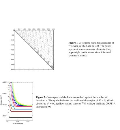
Furthermore, this block matrix is quite sparse, namely the fraction of the non-zero matrix elements is quite small, since the shell-model Hamiltonian in Eq.(3) consists only of one-body and two-body interactions. Figure 1 shows the non-zero matrix elements of the Hamiltonian matrix of44Ti withp f
shell andMπ=0+. ItsM-scheme dimension is 4000. In this case, the fraction of the non-zero matrix elements is around 5%. The fraction is expected to be small in a larger system.
0 500 1000 1500 2000 2500 3000 3500 4000 0
500
1000
1500
2000
2500
3000
3500
4000
Figure 1.M-scheme Hamiltonian matrix of
44Ti withp fshell andM=0. The points
represent non-zero matrix elements. Only upper-right part is shown since it is a real symmetric matrix.
Figure 2.Convergence of the Lanczos method against the number of iteration,n. The symbols denote the shell-model energies ofJπ=0+1 (black
circles) toJπ=0+10(yellow circles) states of
56Ni withp fshell and GXPF1A
interaction [9].
solve the eigenvalue problem. The Krylov subspace is spanned by an initial vector,u, and its products with the matrixHto the power:
Kn(H,u)=span{u,Hu,H2u, ...,Hn−1u}. (5)
In usual shell-model calculations the Lanczos method, one of the Krylov-subspace methods, is used to obtain low-lying eigenvalues. The convergence of the eigenvalue as a function of the number of Lanczos iteration,n, is shown in Fig. 2. The y axis shows the eigenvalues of the Hamiltonian matrix in the Krylov subspace. While the lowest eigenvalue converges quite fast, the high-lying eigenvalue converges slower as the eigenvalue goes higher. At a rough guess, the current limitation of the Lanczos method is that the product of theM-scheme dimension and the number of eigenvectors does not exceedO(1010). While the largest dimension for a few low-lying states are O(1010), the
limitation for the calculation of the level density is much strict: since it requiresO(103) eigenvectors,
the largest dimension becomesO(107). The largest dimension is extended up toO(1010) by utilizing
Figure 3.Schematic view of the contour line in complex planezand its discretized points for the numerical calculations. The red crosses show eigenvalues ofH.
3 Framework of the stochastic estimation of the eigenvalue count
We briefly review the stochastic estimation of eigenvalue density of sparse matrix in this section. This method was introduced and demonstrated in condensed matter physics [7].
For the estimation of the level density, we count the number of the eigenvalues in a specified energy region,Γ. It is given asμ=Tr(PΓ), wherePΓis a projection operator to the subspace spanned by the eigenvectors whose eigenvalues are insideΓ. It is realized by the Cauchy integral as
PΓ= 1
2πi
Γdz
1
z−H
j
wj(zj−H)−1 (6)
whereΓis a contour to surround a certain energy region, or an ovalΓ1in Fig. 3. Although we setΓifor
each energy bin for evaluating the level density, we omit the index of energy binifor simplicity. The contour integral is approximated by a summation of the discretized pointszjshown as blue symbols in
Fig. 3 with the corresponding weightswj. Note that this projector also appears in the Sakurai-Sugiura
method, which is an eigenvalue solver [10, 11].
However, since the trace of Eq.(6) is difficult to calculate directly, we estimate it utilizing Hutchin-son’s estimator [12] as the following equation:
ˆ μ= 1
Ns Ns
i
uT
sPΓus, (7)
whereusis a sample vector whose matrix elements are taken as−1 or 1 randomly. Nsis the number
of sample vectors. While this estimation contains stochastic error, the magnitude of the error depends on the property ofPΓ. For example, if PΓis a diagonal matrix, the stochastic error becomes zero. In preceding works, this estimator gives sufficiently small error even with a small number of sample vectors [7]. In this work, we takeNs=16.
The next step is to evaluateuTsz−1Husby solving a linear equation (z−H)x=us. Since we have
mul-tipleus, we adopt the block conjugate gradient (BCG) method to solve the multiple linear equations
(z−H)X=VwhereVis theD×Nsmatrix whose column isus. We adopt block CG-rQ (BCG-rQ)
method [14] for efficient computation.
WithA=z−H, the BCG-rQ algorithm is shown in Algorithm 1 where qr(V) denotes QR decom-position ofV. TheXk,Pk,Qk, are alsoD×Nsmatrices. The residual matrixQkis orthonormalized
by QR decomposition every iteration to improve the numerical stability [13]. The block algorithm accelerates the convergence and also helps to use a CPU efficiently by increasing contiguous memory access.
However, it requires enormous computational resources to perform the BCG-rQ calculation for eachzjindividually. This problem is overcome by utilizing the shift invariance of the Krylov subspace.
This invariance means that the Krylov subspace of the matrixHis the same as that ofz−H:
Algorithm 1Algorithm of the Block CG-rQ method.
X=O, Q0ρ0=qr(V), Δ0=ρ0, P0=Q0
for k=0,1, ... until ||Δk||< ε||V||
αk=(PHkAPk)−1 Xk+1=Xk+PkαkΔk Qk+1ρk+1 =qr(Qk−APkαk)
Δk+1=ρk+1Δk Pk+1=Qk+1+PkρHk+1
end for
The solution of (z−H)x = u by the CG method is expressed in this subspace, if the number of iterations, n, is large enough. Owing to the shift invariance of the Krylov subspace, the solution of (zj−H)x = ufor any jis also expressed in the same subspace. Thus, by considering this shift
invariance, once we solve (zref−H)X=Vfor a referencezref, we can obtain the solution of (zj−H)X= Vfor anyjwithout further time-consuming matrix-vector products ifnis large enough.
The block Krylov subspace is also invariant with the shiftz:
Kn(z−H,{v1, ..., vNs})=span{v1, ..., vNs,(z−H)v1, ...,(z−H)vNs, ...,(z−H)n−1vNs}=Kn(H,{v1, ..., vNs}).
(9) Therefore, the shift algorithm can also be used for the block CG-rQ method. In practice, shifted block CG-rQ (SBCG-rQ) method is adopted for efficient computations [14]. Finally, the level density is obtained asρ=ΔμE, whereδEis the length ofΓalong the real axis shown in Fig. 3.
The “level density” means a summation of the numbers of levels without counting the degeneracy ofz-component of angular momentum, namely the factor 2J+1. Because of this, especially for even (odd) nuclei, the level density is equal to the eigenvalue density of the Hamiltonian matrix withM=0 (M= 1
2). In order to obtain the spin-dependent level density, we replace the sample vectorvsin Eq.(7)
by the angular-momentum projected vector,PJv s.
The procedure is summarized as follows:
1. Preparezjandwjfor the integral shown in Fig. 3 and Eq.(6).
2. Prepare sample vectorsvs, whose elements are taken as−1 or 1 randomly. If spin-dependent
level density is required, those sample vectors are replaced by the angular-momentum projected vectorsPJvs.
3. Solve linear equations (zj−H)xs,j=usand obtainuTsxs,jby the SBCG-rQ method.
4. Level density is obtained byρ= 1
ΔENs1
Ns s=1
jwjuTsxs,j.
In the present framework, the most time-consuming part is the matrix-vector product in the SBCG-rQ method. The dimension of the vector, theM-scheme dimension, often reaches quite huge and high-performance computing is required. We combine the nuclear shell-model code “KSHELL” [15] and the eigenvalue-solver library “z-Pares” [16], which enable us to utilize state-of-the-art supercomputers efficiently.
4 Benchmark test and level density of
56Fe
In this section, we discuss the level density of 56Fe as a demonstration of the present estimation
Figure 4.Level densities of56Fe against the
excitation energy. These are obtained by stochastic estimation (black line) and by direct counting of the Lanczos results (red line). The experimental values (blue symbols with error bars) are taken from [17]. The energy bin is 0.2 MeV.
calculations, the model space is taken as the p f shell and the GXPF1A interaction [9] is adopted for the realistic effective interaction. This interaction was constructed based on G-matrix interaction and chi-square fitted for the experimental data of low-lying states. TheM-scheme dimension of56Fe
reaches 501,113,392.
The blue symbols with error bars in Fig. 4 show the experimental level density of56Fe obtained
by the Oslo method [17]. The red line shows the exact shell-model level density of56Fe. The exact
values are obtained by the direct counting of the 100 lowest states. The energy bin isΔE=0.2 MeV, and it is the same as the experimental one. The exact Lanczos value shows good agreement the experimental one up to 6 MeV. However, it becomes rapidly difficult to obtain the exact value in higher-energy region since the level density, and hence the number of eigenvalues to be evaluated, increase exponentially.
The black line in Fig. 4 is obtained by the present stochastic estimation withNs =16 and 1550
BCG iteration. This estimation reproduces well the exact value within a certain stochastic error. The estimation is feasible beyond the Lanczos limitation and it reproduces well the experimental value up to 10 MeV. The deviation aroundEx∼9 MeV is considered to be the contribution of negative-parity
states, which is beyond the present model space. As the excitation energy increases, the ratio of the stochastic error to the level density would decrease since the level density increases exponentially and its error is expected to be proportional to the square root of the level density. Further discussion of the error estimation remains for future work.
B. A. Brown and A. C. Larsen also showed the shell-model results of the level density of56Fe by
the direct counting of the Lanczos results in Ref.[18]. They used the same model space and interaction, but the truncation scheme which they applied in order to save computational resources brought about modest underestimation.
5 Removal of the contamination of the center-of-mass motion
Since an atomic nucleus is an isolated system and translational invariance should be taken into account the contamination of center-of-mass motion should be removed in nuclear shell model calculations beyond 0ωmodel space [19]. In order to remove this contamination, we replace the Hamiltonian by
H=H+β(HCM−
3
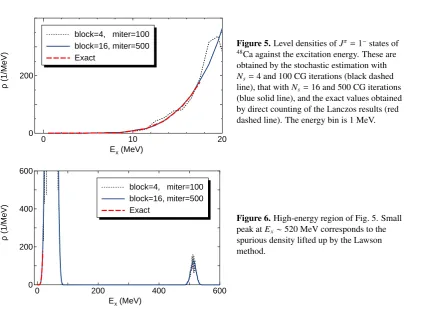
Figure 5.Level densities ofJπ=1−states of
48Ca against the excitation energy. These are
obtained by the stochastic estimation with
Ns=4 and 100 CG iterations (black dashed line), that withNs=16 and 500 CG iterations (blue solid line), and the exact values obtained by direct counting of the Lanczos results (red dashed line). The energy bin is 1 MeV.
2
Figure 6.High-energy region of Fig. 5. Small peak atEx∼520 MeV corresponds to the spurious density lifted up by the Lawson method.
withβω/A=10 MeV.HCMis the Hamiltonian of the center-of-mass motion in a harmonic oscillator
potential whose energy quanta isω. We takeβlarge enough so that the expectation value ofHCM− 3
2ωis close to zero and the excitation of the center-of-mass motion is suppressed. The contaminated
states are lifted up to high-energy region. This prescription is called the Lawson method [20]. Figure 5 shows the level density of Jπ = 1− states of48Ca. The stochastic estimation in shell
model is performed withsd-p f-sdgshells and 1ωtruncation. The level densities are obtained in 1 MeV energy bin. The realistic interaction presently used was introduced in Ref.[21] and provides us with a good description of collective states such as the 3−1 state and the giant dipole resonances of Ca isotopes [22]. The exact value obtained by the Lanczos method is well reproduced by the present estimation withNs=16 and 500 BCG iterations. The estimation withNs=4 and 100 BCG iterations
is shown by the dotted line. Since the number of iterations is small and the BCG does not converge well, it shows pseudo oscillation and disagreement with the exact one.
Figure 6 shows the high-energy region of Fig. 5. The spurious states are lifted up toEx∼520 MeV,
corresponding a small peak in Fig. 6, thereby separated clearly from the main peak. Such separation is also clearly seen even in the dotted line, which is obtained before the convergence.
6 Summary
center-of-mass motion is clearly removed by the Lawson prescription. The present method is feasible up toO(1010) M-scheme dimension, which is a similar order to the limitation to obtain some
low-lying states by the Lanczos method. By adopting this framework, we successfully reproduced the parity equilibration of 2+ and 2− level densities of58Ni in low-energy region in Ref.[8]. Further
applications of this method are in progress.
Acknowledgments
This work has been supported by the HPCI Strategic Program from MEXT, CREST from JST, the CNS-RIKEN joint project for large-scale nuclear structure calculations, and KAKENHI grants (25870168, 23244049, 15K05094) from JSPS, Japan. The numerical calculations were performed on K computer at RIKEN AICS (hp140210, hp150224), FX10 supercomputer at the University of Tokyo, and COMA supercomputer at the University of Tsukuba.
References
[1] W. Hauser and H. Feshbach, Phys. Rev.87, 366 (1952).
[2] H. A. Bethe, Phys. Rev.5, 332 (1936); J. A. Holmes, S. E. Woosley, W. A. Fowler, and B. A. Zimmerman, At. Data Nucl. Data Tables18, 305 (1976); J. J. Cowan, F.-K. Thielemann, and J. W. Truran, Phys. Rep.208, 267 (1991).
[3] Y. Alhassid, G.F. Bertsch, S. Liu and H. Nakada, Phys. Rev. Lett.844313 (2000); H. Nakada, and Y. Alhassid, Phys. Rev. Lett.792939 (1997).
[4] R. A. Sen’kov and V. Zelevinsky, arXiv:1508.03683 [nucl-th]; R. A. Sen’kov and M. Horoi, Phys. Rev. C82024304 (2010).
[5] E. Teran and C. W. Johnson, Phys. Rev. C73024303 (2006).
[6] B. Strohmaier, S. M. Grimes, and S. D. Bloom, Phys. Rev. C 32 1397 (1985); S. M. Grimes, S. D. Bloom, R. F. Hausman Jr., and B. J. Dalton, Phys. Rev. C192378 (1979).
[7] Y. Futamura, H. Tadano and T. Sakurai, JSIAM Lett.3, 61 (2010).
[8] N. Shimizu, Y. Utsuno, Y. Futamura, T. Sakurai, T. Mizusaki and T. Otsuka, Phys. Lett. B753, 13 (2016).
[9] M. Honma, T. Otsuka, B. A. Brown, and T. Mizusaki, Eur. Phys. J. A25, Suppl. 1, 499 (2005). [10] T. Sakurai and H. Sugiura, J. Comput. Appl. Math.159, 119 (2003).
[11] T. Mizusaki, K. Kaneko, M. Honma and T. Sakurai, Phys. Rev. C82, 024310 (2010). [12] M. F. Hutchinson, Commun. Stat., Simulation Comput.,19433, (1990).
[13] A. A. Dubrulle, Elect. Trans. Numer. Anal.12216 (2001).
[14] Y. Futamura, T. Sakurai, S. Furuya, and J. Iwata, VECPAR 2012, LNCS 7851 226 (2013). [15] N. Shimizu, arXiv:1310.5431 [nucl-th]
[16] Y. Futamura and S. Sakurai, http://zpares.cs.tsukuba.ac.jp/ [17] E. Alginet al., Phys. Rev. C78, 054321 (2008).
[18] B. A. Brown and A. C. Larsen, Phys. Rev. Lett.113, 252502 (2014).
[19] E. Caurier, G. Martinez-Pinedo, F. Nowacki, A. Poves, and A. P. Zuker, Rev. Mod. Phys.77427 (2005).
[20] D. H. Gloeckner and R. D. Lawson, Phys. Lett.53B313 (1974).
[21] Y. Utsuno, T. Otsuka, B. A. Brown, M. Honma, T. Mizusaki, and N. Shimizu, Prog. Theor. Phys. Suppl.196, 304 (2012).