Relating Vertex and Global Graph Entropy in
Randomly Generated Graphs
Philip Tee1,2†,‡ ID, George Parisis3‡ ID, Luc Berthouze3‡ ID, and Ian Wakeman3‡ ID*
1 Moogsoft Inc; [email protected] 2 University of Sussex; [email protected]
3 University of Sussex; {g.parisis,l.berthouze,ianw}@sussex.ac.uk
* Correspondence: [email protected];
† Current address: Moogsoft Inc, 1265 Battery Street, San Francisco CA 94111 ‡ These authors contributed equally to this work.
Abstract: Combinatoricmeasuresofentropycapturethecomplexityofagraph,butrelyuponthe calculationofitsindependentsets,orcollectionsofnon-adjacentvertices. Thisdecompositionof thevertexsetisaknownNP-Completeproblemandformostrealworldgraphsisaninaccessible calculation.RecentworkbyDehmeretalandTeeetal,identifiedanumberofalternativevertexlevel measuresofentropythatdonotsufferfromthispathologicalcomputationalcomplexity.Itcanbe demonstratedthattheyarestilleffectiveatquantifyinggraphcomplexity.Itisintriguingtoconsider whetherthereisafundamentallinkbetweenlocalandglobalentropymeasures.Inthispaper,we investigatetheexistenceofcorrelationbetweenvertexlevelandglobalmeasuresofentropy,fora narrowsubsetofrandomgraphs. Weusethegreedyalgorithmapproximationforcalculatingthe chromaticinformationandthereforeKörnerentropy.Weareabletodemonstrateclosecorrelationfor thissubsetofgraphsandoutlinehowthismayarisetheoretically.
Keywords:GraphEntropy,ChromaticClasses,RandomGraphs
1. Introduction and Background
1.1. Overview
Global measures of graph entropy, defined combinatorially, capture the complexity of a graph. In this context complexity is a measure of how distinct or different each vertex is in terms of its interconnection into the rest of the graph. In many practical applications of network science, which can range from fault localization in computer networks to cancer genomics, this difference in connectivity can indicate that certain vertices in a graph are in some way more important to the correct functioning of the network the graph represents. In this paper we explore the potential relationships between vertex level entropy measures and global graph entropy. This is an important problem for a very simple reason. Global graph entropy, as defined originally by Körner [1] is expensive to compute, as it relies upon the calculation of independent sets of the graph. This is a knownNP−Completeproblem, and in most real world graphs the computation of graph entropy is prohibitive. As stated before though, the value of this graph metric though is high, as it fundamentally captures a measure of the complexity of the graph that has a range of practical applications.
If it were possible to approximate the value of graph entropy with a much more easily computable metric, it would make it possible to use entropy in these and potentially many other applications. The fundamental barrier to computability is the fact that the entropy calculation depends upon combinatoric constructs across the whole graph. If instead, a metric were available that was intrinsically local, that is computable for each vertex in the graph with reference to only the local topology of the graph, it would then be possible to efficiently calculate a value for each vertex and then simply sum these values across the graph to obtain an upper bound for the entropy of the graph. The fact
that it is an upper bound is possible to assert by simply appealing to the sub additivity property of graph entropy. That is, for any two graphsG1andG2, the entropy of the union of the graphs obeys
H(G1∪G2)≤H(G1) +H(G2).
Precisely such a metric has been advanced in work by Dehmeret al[2–6], and developed by many other authors including in recent work we published [7] exploring the utility of vertex entropies in the localization of faults on a computer network. The formalisms used by Dehmeret aland in our previous work differ in the construction of the entropies, and how graphs are partitioned into local sets. A primary motivation for this difference was motivated by the practical application of these measures described in [7]. The relation between the vertex entropy formalisms introduced by Dehmer, and global graph entropies have been analyzed [8] and the central focus of this paper is to explore how closely our definitions of vertex entropy approximate global entropies for two classes of Random Graphs, the traditional Gilbert graph [9], and the Scale-Free graphs first advanced by Barabási [10]. We restrict our experimental investigation to simple connected graphs, which in the case of Scale Free graphs arise naturally, for the Gilbert graphs we chose to focus on the Giant Component (GC) of the generated graph. For statistical significance this further restricts the choice of connection probability to a range above the critical threshold at which a GC emerges.
In this section we present an overview of both global and vertex graph entropy, before discussing the experimental analysis in Section2. The data analysis produces a perhaps surprisingly close correlation between vertex and global entropy, which we seek to explain in Section3, by comparing the expected values of Chromatic Information as a proxy for Graph Entropy and the expected values for vertex entropy when considering an ensemble of random graphs. The main result of this paper is that for random graphs the correlation is strong and explained by the co-dependence of both metrics on edge density. We conclude in Section4and point to further directions in this research. In particular, if the correlation we describe in this paper holds as a general result this opens up the use of vertex level measures to frame entropic arguments for many dynamical processes on graphs, including network evolution. Such models of network evolution have been advanced by a number of authors including Petersonet al[11] and ourselves [12].
Before presenting the experimental and theoretical analysis of the possible correlation between local node and global measures of entropy, in the rest of this section we will briefly survey the necessary concepts.
1.2. Global Graph Entropy
The concept of the entropy of a graph has been widely studied ever since it was first proposed by Janos Körner in his 1973 paper on Fredman-Komlós bound [1]. The original definition rested upon a graph reconstruction based upon an alphabet of symbols, not all of which are distinguishable. The construction begins by identifying with each member of an alphabet ofnpossible signalsX= {x1,x2, . . .xn}, with a probability of emissionPi,i∈1, 2, . . . ,nin a given fixed time period. Using this
basic construction the regular Shannon entropy [13] is defined in the familiar way:
H(X) =−
n
∑
i=1Pilog2Pi (1)
are distinguishable. The automorphism groups of this graph are naturally related to the information lost (and hence entropy gained), by certain signals not being distinguishable. To avoid the definition involving complex constructions using these automorphism groups, Mowshowitzet al[15] recast the definition in terms of the mutual information between the independent sets of the graph, where an independent set is equivalent to a chromatic class, that is a collection of vertices that are not adjacent. To establish this definition, let us imagine a process whereby we randomly select a vertex from the graph, according to a probability distributionP(V)for each vertex, which as the process of selection is uniform will be identically 1n for each vertex in a graph of sizen. Each vertex will in turn be a member of an independent setsi∈S(Sis chosen to represent the independent sets to avoid confusion withIthe mutual information). The conditional probabilityP(V|S)is the probability of selecting a vertex when the independent set that it belongs to is known. These probabilities capture important information concerning the structure of the graph. Associated withP(V|S)is a measure of entropy H(V|S), or the uncertainty in the first occurrence of selecting a vertex when the independent set is known. Using these quantities we define Structural Entropy as follows:
Definition 1. The Structural Entropy of a Graph G(V,E), over a probability distribution P(V), H(G,P), is defined as:
H(G,P) =H(P)−H(V|S), (2)
where S is the set of independent sets of G, or equivalently the set of Chromatic Classes.
Closely related to this definition of entropy is Chromatic Information. This is defined in terms of the colorings of the graphs, that divide the graph into subsets ofVwhere each vertex inVhas the same color label. Each graph has an optimal minimum set of colorings which can be achieved, the number of such sets being referred to as the Chromatic Number of the graphχ. These subsets are called
Chromatic ClassesCi, with the constraint thatS
iCi = V. Chromatic information is then naturally defined as:
Definition 2. The Chromatic Information of a graph of n vertices is defined as:
Ic(G) =min {Ci}
"
−
∑
i
|Ci|
n log2
|
Ci|
n
#
, (3)
where the minimization is over all possible collections of chromatic classes, or colorings, of the graph Ci. Crucially, the chromatic information is closely related to the second term in Equation (2),H(V|S), and if we assume that the probability distributionPis uniform, we can relate the two quantities through the following identity.
H(G,P) =log2n−Ic(G) (4)
We will make use of this identity in Section2as chromatic information is much more readily calculable than entropy in standard network analysis packages. It is also common in this measure of information to drop thePinH(G,P), as we are assuming the probability is uniform.
1.3. Local Entropy Measures
where distanced(vi,vj)is the shortest distance between distinct verticesviandvj(i.e. i6= j). For a nodevi∈V, we define, forj≥1, the ‘j-Sphere’ centered onvias:
Sji ={vk ∈V|d(vi,vk) =j} (5) On thesej-Spheres, Dehmer defined certain probability-like measures, using metrics calculable on the nodes such as degree as a fraction of total degree of all nodes in thej-Sphere, from which entropies can be defined. This locality avoids the computationally challenging issues present in the global forms of entropy.
In recent work [7], the authors extended this definition to introduce some specific local measures for Vertex Entropy, that is the graph entropy of an individual node in the graph. The analysis that was followed was based upon the concept of locality introduced in Dehmeret al, using the concept of a j-Sphere. In this work we will expand upon that analysis, and, instead consider the vertices of a graph as part of an ensemble of vertices, and the graph itself in turn as part of an ensemble of Graphs. Returning to the fundamental definition of entropy, it is a measure of how incompletely constrained a system is microscopically, when certain macroscopic properties of the system are known. For example, if we have an ensemble of all possible simple, connected graphs of orderN,G(N), (that is|V|=N), we potentially have a very large collection of graphs. Further, we could go on to prescribe a further property such as average node degreehkifor the whole ensemble, and ask what is the probability of randomly selecting a member of the ensembleGi(N) ∈ G(N), that shares a given value of this propertyhki, and denote that asP(Gi). Following the analysis in Newmanet al[16] we can then define the Gibbs entropy of the ensemble as:
SG(N)=−
∑
Gi∈G(N)
P(Gi)log2P(Gi), (6)
which is maximized subject to the constraint, ∑
Gi∈G(N)
P(Gi)hkii=hki. This analysis allows us to go from the observed valuehkito the form of degree distribution and then on to other properties for the whole ensemble. In essence in our work, we take a different approach in two regards. Firstly, we restrict ourselves to the vertex level, where we consider that the vertices of an individual graph are themselves a randomized entity, which can be assembled in many ways to form the end graph. For example, if we were to decompose a given graph into the degree sequence of the nodes, there will be many nodes of the same degree, which does not completely prescribewhichnode in the graph we are considering. In that way a measure of uncertainty and therefore entropy naturally arises.
The second difference to the approach taken by Newman et al, is that rather than work from a measurable constraint and maximized form of entropy back to the vertex probability, we ask what probabilities we can prescribe on a vertex. In the interests of computational efficiency we construct a purely local theory of the graph structure constrained to those vertex properties that are measurable in the immediate (that isj = 1) neighborhood of the vertex. Out of the possible choices we have selected node degree, node degree as a fraction of the total edges in the network, and local clustering coefficient. In our work, we also redefined the local clustering coefficientCi
1of a nodeias the fraction
• Inverse DegreeIn this case we denote the vertex probability as:
P(vi) = Z kα
i
, with (7)
Z−1=
∑
j k−α
j to ensure normalization. (8)
This type of vertex probability mirrors the attachment probability of the scale free model and leads to a power law of node degree. In the standard scale free modelα=3, but for the purposes
of our experimentation, and for simplicity, we setα = 1. In essence very large hubs are less
probable, which intuitively captures the notion that they carry more of the global structure, and therefore information, of the graph. Graphs comprised of nodes with similar degrees will maximize entropy using this measure, reflecting the fact less information is carried by knowledge of the node degree.
• Fractional DegreeWe use in this case the following for vertex probability:
P(vi) = ki
2|E|. (9)
This probability measure captures the likelihood that a given edge in the network terminates or originates at the vertexvi. Nodes with a high value of this probability will be more highly connected in the graph, and graphs which have nodes with identical values of the probability will have a higher entropy. This reflects the fact that the more similar nodes are the less information is known about the configuration of a given node by simply knowing its fractional degree. • Clustering CoefficientThe clustering coefficient measures the probability of an edge existing
between the neighbors of a particular vertex. However, its use in the context of a vertex entropy needs to be adjusted by a normalization constantZ =∑iCi1to be a well behaved probability measure and sum to unity. For simplicity we omit this constant and we assert:
P(vi) =Ci1 (10)
The local clustering coefficient captures the probability that any two neighbors of the nodevi are connected. The larger this probability the more the local one hop subgraph centered atviis to the perfect graph. Again graphs comprised of nodes with similar clustering coefficient will maximize this entropy, reflecting the fact that the graph is less constrained by knowledge of the nodes clustering coefficients.
In essence for a given graphG(N)∈G(N), we specify a measured quantity for vertexvi, asx(vi) =xi, and ask what is the probability of a random vertexvihaving this value. We denote this probability as P(vi)x(vi)=xi. This allows us to define entropy at the vertex level , and for the whole graph as:
S(vi) =−P(vi)log2P(vi) (11) S(G) =−
∑
vi∈G
P(vi)log2P(vi) (12)
In our analysis we compute the values of each of these variants of vertex entropy, summed across the whole graph as described in Equation12. Because of the local nature of the probability measures the vertex entropy values are far quicker to compute than any of the global variants, and do not involve any knownNP−Completecalculations. In Section2we describe the approach taken to perform this analysis. The results indicate that the vertex entropy approximation yields a value that is closely correlated with the global values of chromatic information (and therefore entropy).
2. Experimental Analysis
2.1. Method and Objectives
We seek to establish whether there is any significant relationship between the global graph entropy of a graph, and the entropy obtained by summing the local node values of entropy. Because of the computational limits involved in calculating global values of entropy, we are restricted to graphs of moderate size, which rules out analyzing repositories of real world graphs such as the Stanford Large Network Dataset [17], or the Index of Complex Networks (ICON) [18]. A more tractable source of graphs are randomly generated graphs, where we can control the scale.
Random graphs are well understood to replicate many of the features of real networks, including the ‘small world’ property, clustering and degree distributions. We consider in our analysis two classes of randomly generated graphs, the Gilbert Random GraphG(n,p)[9], and the scale-free graphs generated with a preferential attachment model [10]. For both types of graphs we simulated a large number of graphs with varying parameters to generate many possible examples of graphs that share a fixed number of vertices, with the choice of Gilbert graphs permitting varying edge counts and densities. For the purposes of our analysis we fixed the vertex count atn=|V|=300 and in each case we included only fully connected, simple graphs. For the Gilbert graphs, this entailed analyzing only the Giant Component (GC) to ensure a fully connected graph.
We will discuss the results for each type of graph in more detail below, but the data revealed a close correlation between the chromatic information of the graph (and therefore structural entropy), and the value obtained by summing the local vertex entropies. We considered three variants of the vertex entropy and also included the edge density of the graph, defined as:
C(G) = 2|E|
n(n−1). (13)
This measures the probability of an edge existing between any two randomly selected vertices. To quantify the nature of the relationship between each of the aforementioned local entropies (including edge density) and chromatic information of the graphs, we adopted a model selection approach by performing polynomial regression using polynomials of increasing order up to 5, referred to asH1,...,5henceforth, using the technique of least squares to numerically calculate the polynomial
coefficients. The best model (within the family of models considered) was assessed based on the Bayesian Information Criteria (BIC), and Akaike Information Criteria (AIC) [19].
To calculate the measures we make the assumption that the distribution of the errors are identically and independently distributed, and reduced the likelihood function to the simpler expressions:
BIC=nloge(σˆr2) +klogen (14)
AIC=nloge(σˆr2) +2k (15)
ˆ
σr2= 1
n i=n
∑
i=1(yiˆ −yi)2, (16)
(17)
where ˆyiis the prediction by modelH, ˆσr2is the residual sum of squares,kthe number of parameters
in the model (in this case forHj,k=j+1), andnthe number of data points.
2.2. Scale-Free Graphs
The data for the scale-free graphs is displayed in Figure 1. We have segregated the plots by the calculated chromatic number for the graphs, and overlaid the optimal least squares fit model. It is suggestive that for graphs that share the same value ofχ, there is a non-trivial relationship between
the metrics. To gain insights into the nature of this relationship, the data was fitted using a least squares approach to polynomials up to the 5thdegree. In Tables1,2,3,4we applied both the Bayesian Information Criteria and Akaike Information Criteria to identify the best model. We have highlighted the row for the model with the strongest performance in the BIC test, and the∆BIC/∆AICis measured from theH1model which performs worse in both analyses. In each case there is strong support for
the existence of a relationship between the vertex entropy measures and chromatic information. Both AIC and BIC have a marginal preference for higher order polynomial models, with rejection of higher order indicating a preference forH2for Inverse Degree and Edge Density. The other measures require
higher order fitting, overH4, being necessary for Fractional Degree andH3for Cluster Entropy.
Model Bayes Information Criteria ∆BIC Akaike Information Criteria ∆AIC
H1 -734.33 0.00 -740.33 0.00
H2 -830.12 -95.80 -839.14 -98.80
H3 -825.16 -90.84 -837.18 -96.85
H4 -821.95 -87.62 -836.97 -96.63
H5 -818.63 -84.31 -836.66 -96.32
Table 1.Model Selection Analysis for Inverse Degree Entropy for Scale-Free Graphs of constant|V|
Model Bayes Information Criteria ∆BIC Akaike Information Criteria ∆AIC
H1 -708.84 0.00 -714.84 0.00
H2 -715.24 -6.41 -724.25 -9.41
H3 -719.49 -10.66 -731.51 -16.66
H4 -719.62 -10.79 -734.64 -19.80
H5 -715.31 -6.47 -733.33 -18.49
Table 2.Model Selection Analysis for Fractional Degree Entropy for Scale-Free Graphs of constant|V|
Model Bayes Information Criteria ∆BIC Akaike Information Criteria ∆AIC
H1 -728.34 0.00 -734.35 0.00
H2 -796.47 -68.12 -805.48 -71.13
H3 -798.84 -70.50 -810.86 -76.51
H4 -794.89 -66.54 -809.90 -75.55
H5 -793.77 -65.43 -811.80 -77.44
Table 3.Model Selection Analysis for Cluster Entropy for Scale-Free Graphs of constant|V|
Model Bayes Information Criteria ∆BIC Akaike Information Criteria ∆AIC
H1 -777.77 0.00 -783.78 0.00
H2 -844.94 -67.17 -853.96 -70.18
H3 -842.39 -64.62 -854.40 -70.63
H4 -839.21 -61.43 -854.23 -70.45
H5 -836.87 -59.10 -854.89 -71.11
(a)Inverse Degree (b)Fractional Degree
(c)Clustering Coefficient Entropy (d)Edge Density
Figure 1. Sum of vertex entropies for whole graph vs. chromatic information for Barabási-Albert scale-free graphs of constant|V|.
2.3. Gilbert Random Graphs G(n,p)
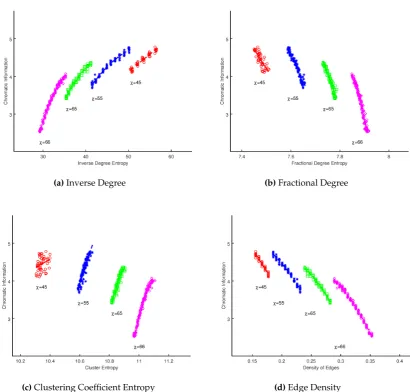
In addition to scale-free graphs we analyzed random graphs. The results are displayed in Figure
2, overlaid with the least squares optimized best fit. On visual inspection it appears that there is a systematic and non-trivial relationship between the metrics. In order to gain insights into this relationship, the data was again fitted using a least squares approach to polynomials up to the 5th degree. In Tables5,6,7,8we applied both the Bayesian Information Criteria and Akaike Information Criteria to select the best model (among the models considered). As in the case of the scale-free graphs, we have highlighted the row in bold corresponding to the best model from a BIC perspective, and
∆BIC/∆AIC, is measured against the worst performing modelH1. For Gilbert graphs, AIC and BIC
both support the hypothesis of a relationship between the metrics. In the case of all but Inverse Degree, it would appear thatH2is an optimal choice of model. Inverse Degree, however would appear to be
Model Bayes Information Criteria ∆BIC Akaike Information Criteria ∆AIC
H1 -2004.92 0.00 -2008.75 0.00
H2 -2181.68 -176.76 -2189.33 -180.59
H3 -2182.62 -177.70 -2194.10 -185.35
H4 -2176.82 -171.90 -2192.12 -183.37
H5 -2171.14 -166.22 -2190.27 -181.52
Table 5.Model Selection Analysis for Inverse Degree Entropy for Random Graphs of constant|V|
Model Bayes Information Criteria ∆BIC Akaike Information Criteria ∆AIC
H1 -1806.14 0.00 -1809.96 0.00
H2 -1874.29 -68.15 -1881.94 -71.98
H3 -1868.70 -62.56 -1880.17 -70.21
H4 -1859.34 -53.20 -1874.64 -64.68
H5 -1856.25 -50.11 -1875.38 -65.42
Table 6.Model Selection Analysis for Fractional Degree Entropy for Random Graphs of constant|V|
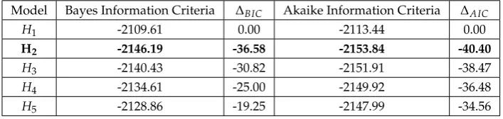
Model Bayes Information Criteria ∆BIC Akaike Information Criteria ∆AIC
H1 -2109.61 0.00 -2113.44 0.00
H2 -2146.19 -36.58 -2153.84 -40.40
H3 -2140.43 -30.82 -2151.91 -38.47
H4 -2134.61 -25.00 -2149.92 -36.48
H5 -2128.86 -19.25 -2147.99 -34.56
Table 7.Model Selection Analysis for Cluster Entropy for Random Graphs of constant|V|
Model Bayes Information Criteria ∆BIC Akaike Information Criteria ∆AIC
H1 -951.67 0.00 -955.49 0.00
H2 -985.93 -34.26 -993.58 -38.08
H3 -980.15 -28.48 -991.63 -36.13
H4 -974.37 -22.71 -989.68 -34.18
H5 -969.80 -18.13 -988.93 -33.43
Table 8.Model Selection Analysis for Edge Density for Random Graphs of constant|V|
3. Theoretical Discussion of the Results
The strong correlation between chromatic information and the various forms of vertex entropy derived graph entropies may at first seem paradoxical. The first quantity is combinatorial in nature, and depends upon the precise arrangement of edges and vertices to produce the optimal coloring which dictates its value. The summed vertex entropies, at least to first order, depend solely upon the individual node degrees and take little or no account of the global arrangement of the graph.
It is certainly beyond the scope of this work, and indeed to the opinion of the authors, intractable to calculate a precise relationship between the two quantities. It is possible, however, to construct an argument as towhythe two quantities might be in such close correlation.
(a)Inverse Degree (b)Fractional Degree
(c)Clustering Coefficient Entropy (d)Edge Density
consider an ensemble of graphsG(G(V,E)), with degree distributionsP(k), and fixed ordern=|V|. For this ensemble, a random memberGof ordern, of chromatic numberχ(G)will have an average
chromatic information as follows:
hIC(G)i ≈ −χ(G)×
h|Cα|i
n log2 h|Cα|i
n (18)
whereh|Cα|i, is the average size of the chromatic class.
Using the definitions of vertex entropy described in Section1, we can also similarly compute an average value of each vertex entropy for a member of the ensembleG, where we have taken the continuum approximation in the integral on the r.h.s:
hSvertexi=n× hS(vi)i=n Z ∞
1 P
(k)S(k)dk (19)
In the case of the scale free graphs, this yields analytically soluble integrals for inverse degree, fractional degree vertex entropies, and edge densities but for the clustering coefficient entropies, and for all G(n,p)random graphs the integrals are not solvable directly. To simplify the analysis we use the approximate continuum result for the scale free degree distributions att→ ∞,P(k) = 2km32, where
mis the number of nodes a new nodes connects to during attachment. For the clustering coefficient we can make a very rough approximation in the case of scale free networks of 4m/nby arguing that for an average node degree ofhki = 2m, each of the neighbors shares the average degree and has a probability if 2m/nof connecting to another neighbor of the vertex. The quantity is not exactly calculable, but in [10] a closer approximation givesC1i ∝n−3/4, though for simplicity we will use our rough approximation. Where an exact solution is not available we can roughly approximate the value ofhS(vi)i, by replacing the exact degree of the node by the average degree and then asserting:
hSvertexi=n×S(hki) (20)
We summarize these expressions in Table9
Vertex Entropy Measure Scale Free Graphs Random Graphs
G(n,p) Inverse Degree 2nm2/9 ln 2 p−1log2(pn) Fractional Degree mlog2(2mn) log2n
Clustering Coefficient 4mlog2(n/4m) −nplog2p
Table 9.Average Entropies across Random Graphs
In section2we presented the analysis of samples of randomly generated graphs created using three schemes. Each of these showed a surprisingly strong correlation between the vertex entropy measures, summed across the whole graph, and the chromatic information obtained using the greedy algorithm. The greedy algorithm is well known to obtain a coloring of an arbitrary graph which is close, but not optimal. Indeed the chromatic number of the graph obtained from the greedy algorithmχg(G)is an
upper bound of the true chromatic numberχ(G). For a full description see [9,20].
3.1. Gilbert Random Graphs
Let us first consider the case of the Gilbert random graphs. We follow the same treatment and notation as in [9] and [21]. We construct the graph starting withnvertices, and each of the 12n(n−1)
possible links are connected with a probabilityp. The two parametersnandpcompletely describe the parameters of the generated graph graph, and we denote this family of graphs asG(n,p). It is well known that equation (18) is maximized when each of the chromatic classes of the graphCαare uniform.
That is, if the cardinality fo a chromatic class is denoted by|Cα|, andχis the chromatic number of the
|Cα|=
n
χ,∀Cα (21)
This chromatic decomposition is only obtained from the perfect graph onnvertices,Kn, and proof of this upper bound is outlined in [7]. For a given random graphG(n,p), we denote the coloring obtained in this way, the homogenized coloring ¯CαofG(n,p), and we assert thatIC(G)≤ IC¯ (G). It is
straight forward to verify that this yields as an expression for the chromatic information the following:
IC(G)≤IC¯ (G) =logχ (22)
To build upon the analysis, we consider a randomly selected chromatic classCα, which hasc = χn
nodes. We denote the probability thatcrandomly selected nodes do not posses a link between them as ¯P(Cα,χ), and the probability thatat least one link exists between these nodes asP(Cα,χ). We
consider a large ensemble of random graphs, generated with the same Gilbert graph parametersn,p, which we write asG(n,p). For a randomly chosen member of this ensemble, the criteria for the graph G(n,p)∈ G(n,p)to possess a chromatic numberχ, is simply that it is more likely forcrandomly
selected nodes inG(n,p)to be disconnected. That is: ¯
P(Cα,χ)≥P(Cα,χ) (23)
To estimate the first term, we note that forcrandomly chosen nodes to have no connecting edges is given by:
¯
P(Cα,χ) = (1−p)
1
2c(χ)(c(χ)−1) (24)
For brevity of notation we writec(χ)asc, and ask the reader to remember thatcis a function of the
chromatic number of the graph. We can also estimate the second term, by factoring the probability of a link from any of the nodesvi ∈ Cα, connecting to another node inCα. The total probability is
accordingly the product of:
P(Cα,χ) =P(of any link)×P(link connects two nodesvi,vj ∈Cα)×c
Feeding in the standard parameters from the Gilbert graphs, we obtain:
P(Cα,χ) =p×
c(c−1)
n(n−1)×c = pc
2(c−1)
n(n−1)
fornc,≈ pn χ3
If we substitute back in the dependence ofcupon the chromatic number, we obtain the following inequality, as the criteria for a given chromatic numberχto support an effective random coloring of
the graph, we obtain the following inequality that can be used to estimateχ:
(1−p)12c(c−1)≥ pc
2(c−1)
n(n−1) (25)
It is easy to verify that equality is only ever reached whenp→1, which yields the perfect graph in whichc=1, as every node is adjacent to every other node. The left hand side of Equation(25) is an increasing function ofχ, whereas the right hand side is a decreasing function, so asχincreases we
estimate of the value. Although Equation (25) as a transcendental equation is not directly soluble, we can numerically solve to determine the value ofχfor a fixed link probabilitypat which equality is
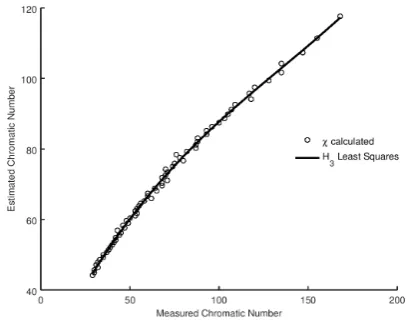
reached. We present the results of the analysis in Figure3, together with the optimal least squares fit of the relationship. We can also evaluate the best model for the relationship between our estimate and the measured values using BIC and AIC in the same manner as with the metrics. We present the results in Table10. It is evident that a cubic relationship offers the best choice of model, and that fit is overlaid on the experimental data in Figure3.
Model Bayes Information Criteria ∆BIC Akaike Information Criteria ∆AIC
H1 -90.00 0.00 -92.25 0.00
H2 -138.79 -48.79 -143.28 -51.04
H3 -146.53 -56.53 -153.28 -61.03
H4 -142.72 -52.72 -151.71 -59.47
H5 -138.60 -48.60 -149.84 -57.59
Table 10.Model selection analysis for computedχversus measured for|V|=300.
Figure 3.Calculatedχversus measuredχ, for Gilbert graphsG(n,p)withn=300 andp∈[0.3, 1.0,].
Overlaid is the Least Squares Fit forH3.
Having established that we can use Equation (25) to generate a good estimate of the chromatic number of a Gilbert graph, we can now attempt to explain how the chromatic information obtained from the greedy algorithm correlates with the vertex entropy measures. We begin by simplifying Equation (25) to determine the minimum value ofχat which equality is reached, by assuming the limit ofcn,
andc,n1 to obtain:
(1−p) n2 2χ2 = pn
χ3
Taking the logarithm of both sides of this equation and manipulating we arrive at the following expression:
3 logχ=logpn− n 2
2χ2log(1−p) (26)
¯ ICG=
1
3logpn− n2
6χ2log
Equation27represents an approximation for the chromatic information of a random graph. Numerical experimentation indicates that the first term dominates for small values ofp, and asp→1.0 the second terms becomes numerically larger. Inspection of Table9, shows that Equation27contains terms that reflect a number of the expressions for the vertex entropy quantities we have considered. Indeed as the experiments were conducted at a fixed value ofn=300, for smallp, by elementary manipulation one can see that ¯ICG∝pSVE, or alternatively ¯ICG∝SCE/p. Although this is a far from rigorous analytical derivation of the dependence of the chromatic information on the vertex entropy terms, the analysis does perhaps go some way to making the close correlation experimentally make sense in the context of this theoretical analysis. Deriving an exact relationship between the two quantities is beyond the scope of this work.
3.2. Scale free graphs
In the case of scale free graphs we can follow a similar analysis to the pure random case. To derive the probability of a link, for a randomly selected node the average probability of attachment p=hki/2mt by appeal to the original preferential attachment model. The dependence upon the connection valence mdrops out and the average probability of a link existing between two nodes becomesp=1/n. Following an identical argument to the random graph case we arrive at the following relationship:
¯ ICG=
n2 4χ2log2
n n−1
!
(28)
Again, it is important to stress that this is not a rigorous derivation of a relationship between chromatic information and vertex entropy, but it is possible to explain some of the structure in the results presented in Figure1. For a given fixed value ofχthe experiments represent graphs produced with
increasing edge densities. As edges are added to the graph thatdo notincrease the chromatic number, the size of the chromatic classes will evidently equalize (a discussion of this point can be found in [7]). This will have the effect if increasing the chromatic information, until a point is reached where
χ→χ+1. At this point the denominator of Equation28will increase causing a drop in chromatic
information. So, as each vertex entropy measure is fundamentally dependent upon the number of edges in a fixed sized graph, we would expect to see a series of correlations for each value of chromatic information, which is indeed what is demonstrated in Figure1.
4. Conclusion
In this work we have principally been interested in investigating what, if any, correlation exists between purely local measures of graph entropy and global ones. It is not possible to make a general statement that for any graph this correlation exists, but for the two classes of random graphs considered it is persuasive that a relationship exists.
1. Körner, J. Fredman–Komlós bounds and information theory, 1986.
2. Dehmer, M. Information processing in complex networks: Graph entropy and information functionals.
Applied Mathematics and Computation2008,201, 82–94.
3. Dehmer, M.; Mowshowitz, A. A history of graph entropy measures. Information Sciences2011,181, 57–78. 4. Mowshowitz, A.; Dehmer, M. Entropy and the complexity of graphs revisited. Entropy2012,14, 559–570. 5. Cao, S.; Dehmer, M.; Shi, Y. Extremality of degree-based graph entropies. Information Sciences2014,
278, 22–33.
6. Emmert-Streib, F.; Dehmer, M.; Shi, Y. Fifty years of graph matching, network alignment and network comparison. Information Sciences2016,346-347, 180–197,[1410.7585].
7. Tee, P.; Parisis, G.; Wakeman, I. Vertex Entropy As a Critical Node Measure in Network Monitoring.IEEE Transactions on Network and Service Management2017,14, 646–660.
8. Dehmer, M.; Mowshowitz, A.; Emmert-Streib, F. Connections between classical and parametric network entropies.PLoS ONE2011,6, 1–8.
9. Bollobás, B.Random Graphs, 2nd ed.; Cambridge University Press, 2001.
10. Albert, R.; Barabási, A.L. Statistical mechanics of complex networks.Review of Modern Physics2002,74. 11. Peterson, J.; Dixit, P.D.; Dill, K.A. A maximum entropy framework for nonexponential distributions.
Proceedings of the National Academy of Sciences2013,110, 20380–20385,[arXiv:1501.01049v1].
12. Tee, P.; Wakeman, I.; Parisis, G.; Dawes, J.; Kiss, I.Z. Constraints and Entropy in a Model of Network Evolution2016. [1612.03115].
13. Shannon, C.E. A Mathematical Theory of Communication. The Bell System Technical Journal1948,
27, 379–423.
14. Simonyi, G. Graph entropy: a survey. Combinatorial Optimization1995,20, 399–441.
15. Mowshowitz, A.; Mitsou, V. Entropy, Orbits, and Spectra of Graphs. Analysis of Complex Networks: From Biology to Linguistics2009, pp. 1–22.
16. Park, J.; Newman, M.E.J. Statistical mechanics of networks. Physical Review E - Statistical, Nonlinear, and Soft Matter Physics2004,70, 1–13,[arXiv:cond-mat/0405566].
17. Leskovec, J.; Krevl, A. SNAP Datasets: Stanford Large Network Dataset Collection. http://snap.stanford.edu/data, 2014.
18. Clauset, A.; Tucker, E.; Sainz, M. The Colorado Index of Complex Networks. http://icon.colorado.edu/, 2016.
19. Burnham, K.P.; Anderson, D.R. Multimodel inference: Understanding AIC and BIC in model selection.
Sociological Methods and Research2004,33, 261–304,[arXiv:1011.1669v3].
20. Bollobàs, B.Modern Graph Theory; Springer-Verlag New York, 1998; pp. XIV, 394.
21. Barabási, A.L.Network Science; Cambridge University Press; 1 edition (August 5, 2016), 2016; p. 474. 22. Trugenberger, C.A. Quantum gravity as an information network self-organization of a 4D universe.Physical
Review D - Particles, Fields, Gravitation and Cosmology2015,92, 1–12,[1501.0140].
![Figure 2. Sum of vertex entropies for whole graph vs. chromatic information for Gilbert graphs G(n, p)for p ∈ [0.31, 0.7].](https://thumb-us.123doks.com/thumbv2/123dok_us/8015561.1332779/10.595.98.518.181.602/figure-vertex-entropies-graph-chromatic-information-gilbert-graphs.webp)