Efficient Automatic Engineering Design Synthesis Via Evolutionary Exploration

(1)

Exploration

Thesis by Cin-Young Lee

In Partial Fulfillment of the Requirements for the Degree of

Doctor of Philosophy

California Institute of Technology Pasadena, California

2002

(2)

©

2002

(3)

Acknowledgements

There are a great many people that I need to thank and acknowledge for their part in this thesis. First, I would like to thank my advisor, Professor Erik K. Antonsson, whose laissez-faire approach to graduate guidance was greatly appreciated because it allowed me to explore freely, which meant, equivalently, that I could learn about the things I enjoy. Learning became fun for me once again and, in my opinion, that's what education should be. Unfortunately, it took me some two decades to regain this childhood joy_

My parents deserve special thanks. Without their love and support I could never have come so far. I hope these two simple sentences can convey the magnitude of my grati!ude. I also thank them deeply for giving me Cin-Ty, my brother. He has taught me more than he knows, as he has been a model to which I have often aspired.

(4)

Foreword

Everything has a story and this is the story of how this thesis came to be. It is my personal opinion that much can be learned through history to clarify the present. My hope is that by describing the events that culminated in the completion of this thesis that the work will have some context and relevance. Because, in contrast to the cliche, it's not only about where you get, but how you get there. After all, results are useless if they cannot be replicated.

Throughout the early years of my tenure at Cal, I did not have any idea what I wanted to do. Sure, I was a mechanical engineering and materials science major, but, like most undergraduates, I didn't know what I was getting into when I chose those majors. By the time I did know, it was too late to change. So, in the summer of my junior year, I went off to Sandia National Labs to work with Dr. Robert W. Schwartz, now a professor at Clemson University, on pyroelectric PZT thin films. I decided then that, as a future career, I would like to be in the microelectronics field since it seemed to be a hot and lucrative field. Unfortunately, my education was not well suited to the choice I had made.

After returning to Cal for my senior year, I began working with Prof. George C. Johnson and his student Peter T. Jones. To my great surprise and joy, our research focused on MEMS - a popular new microelectronics technology that was ideally suited to study by mechanical engineers and material scientists. That decided it. My graduate career would focus on MEMS research. With this goal in mind, I went to Michigan to study under Prof. Liwei Lin who, at the time, was an up and coming star of the MEMS arena. Michigan was a great place and I met some amazing people, but I could not handle the cold winters of Michigan and I missed sunny California. So, I asked Prof. Erik Antonsson if he would consider re-admitting me to Caltech: Thankfully, he said yes and I was on my way to Caltech to study MEMS.

(5)

continue our current research directions.

A senior graduate student, by the name of Hui "Frank" Li, laid the groundwork of our current MEMS research efforts by developing a mask-layout synthesis tool that implemented a genetic algorithm (in fact, an earlier student, Ted Hubbard, was the first in Erik's group to study MEMS in some manner). As I was to be continuing Frank's work, I had to understand how genetic algorithms worked. At first, I was a bit apprehensive (I mean what does a mechanical engineer know about biology?), but as I began learning more about genetic algorithms and evolutionary computation in general, my interest in the subject grew.

I along with another student, Lin Ma, who was my senior, were given the task of improving the shortcomings of Frank's work. At least initially, Lin and I worked on two separate lines of research. His research emphasized the introduction of multiple processes into the mask-layout synthesis application; whereas I tried to remove the restriction of fixed number of polygon vertices. This began my interest in the tool rather than the application, since the application, it seemed to me, was only a specialized instance of the tool. Of course, by tool I mean evolutionary computation. So, I began studying evolutionary computation in earnest and tried to develop a general variable length chromosome representation. This fortuitously led to my work with non-coding segments and linkage learning, which further led to the development of the speciation mechanisms in this thesis. In fact, if one has a keen eye, they should no doubt see the relations amongst all of these before I describe the issue near the end of my thesis.

There are two "morals" I hope the reader will take from this story. The first is that my choices were guided in some manner, a selection if you will. Second, there were chance encounters that led me to my fortunate coincidences. In fact, one might say that this thesis evolved from earlier ideas.

(6)

Abstract

The evolution of designs in nature has been the inspiration for this thesis, which seeks to develop a framework for efficient automatic engineering design synthesis based on evolutionary methods.

The design synthesis process is equated to an evolutionary process. Because of this, the same formalization for evolution, the evolution algorithm, is used as a design synthesis formalism. Im-plementation of the evolution algorithm on a computer allows evolution of non-biological systems, and, hence, automatic engineering design synthesis. The early and canonical versions of such evo-lutionary computation are bare bones evolution tools that neglect several key aspects of evoevo-lutionary systems. Some universal aspects of good designs are identified, three of which are dealt with in this thesis. These are variable complexity, modularity, and speciation.

Framed in an evolutionary context, each of these characteristics are requisites for being able to evolve in correspondence with a dynamic environment. Those that are most evolvable will survive.

After all, if a species cannot evolve quickly enough with changes in the environment, it will perish. In a design context, this indicates that the characteristics are vital for efficiency and shorter design cycles.

(7)

List of Figures

4.1 Test Problem I with L = 50. Proof of concept test case for variable length search. 24

4.2 Test Problem 2 with L

=

50. Trade-off test case for variable length search. 25

4.3 Non-touching cluster data set and corresponding partitions. . 32

4.4 Non-touching cluster data set and typical evolved partitions. 32

4.5 Actual (-) and typical evolved partitions (- -) for non-touching case. Actual (x) and typical

evolved (8) cluster centers. . . 33

4.6 Touching cluster data set and corresponding partitions. 34

4.7 Touching cluster data set and typical evolved partitions. 34

4.8 Actual (-) and evolved partitions (- -) for touching case. Actual (x) and typical evolved (8)

cluster centers. . . .

4.9 Target shape and best shape for Generation l.

4.10 Best shapes for Generation 15 and 25 . .

4.1 T Best shapes at generations 65 and 105 ..

35 40 40 41

5.1 Diagram of the non-coding representation. . . . . 47

5.2 Diagram of the parallel linkage characteristics that overlapping range representations can

exhibit. . . 49

5.3 Royal Road function modules. . 50

5.4 Gene indices for the first chromosome that matches a module of the given Royal Road

module level. . . 53

5.5 Average generation at which each level is discovered for population size of 100. . 54

5.6 Example of a feedforward artificial neural network. . . . 56

5.7 (a) Connection cycle. (b) 2-D index ranges needed to encode connection topology of (a). 58

5.8 (a) Connection cycle with additional node. (b) 2-D index ranges needed to encode

(11)

5.9 Connection cycle with 2 additional nodes that cannot be encoded by any combination of

2-D index ranges. . . . . 60

5.10 Parent I. (a) Network topology. Connections are determined from overlapping index ranges

shown in (b) and weights are proportional to signed Pi difference. (b) Index ranges for each

node . . . .

5.11 Parent 2. (a) Positions and network topology. (b) Index ranges for each node.

5.12 Overlay of Parents I and 2. (a) Positions and network topology. Parent 1 denoted by gray

nodes and integers. Parent 2 denoted by black nodes and letters. (b) Index ranges for each

node. Crossover range denoted by the bold rectangle. . . . .

5.13 Offspring I. (a) Positions and network topology. (b) Index ranges for each node.

5.14 Offspring 2. (a) Positions and network topology. (b) Index ranges for each node.

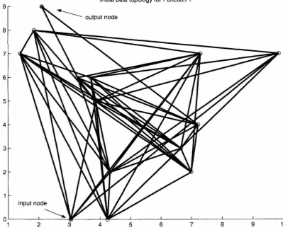
5.15 Initial best ANN topology for Function I (y

=

x) using uniform range crossover. Weights

61 63

64 65

66

determined from difference in horizontal values. Node layer denoted by vertical axis. . . . 70

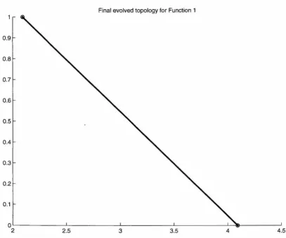
5.16 Final evolved ANN topology for Function I (y

=

x) using uniform range crossover. Axes are as in 5.15. . . . . 71

5.17 Function I (y = x) data, initial best approximation, and final evolved approximation using

uniform range crossover. 72

5.18 Initial best ANN topology for Function 2 (tanh(x

+

2)) using uniform range crossover. Axes are as in Figure 5.15. . . . 73

5.19 Final evolved ANN topology for Function 2 (tanh(x

+

2)) using uniform range crossover.

Axes are as in Figure 5.15. . . . 74

5.20 Function 2 (tanh(x

+

2)) data, initial best approximation, and final evolved approximation

using uniform range crossover using uniform range crossover. . . . . . . . . 75

5.21 Initial best ANN topology for Function 3 (sin(x)) using uniform range crossover. Axes are

as in Figure 5.15. . . . . 76

5.22 Final evolved ANN topology for Function 3 (sin(x)) using uniform range crossover. Axes

are as in Figure 5.15. . . . . 77

5.23 Function 3 (sin(x)) data, initial best approximation, and final evolved approximation using

uniform range crossover. . . . 78

5.24 Initial best ANN topology for Function 4 (cos(x)) using uniform range crossover. Axes are

(12)

5.25 Final evolved ANN topology for Function 4 (cos(x) using uniform range crossover. Axes

are as in Figure 5.15. . . . . 80

5.26 Function 4 (cos(x» data, initial best approximation, and final evolved approximation using

uniform range crossover. 81

5.27 Initial best ANN topology for Function 5 (y

=1

x

I).

Axes are as in Figure 5.15. . 82

5.28 Final evolved ANN topology for Function 5 (y

=

1

x

I).

Axes are as in Figure 5.15. 83

5.29 Function 5 (y

=1

x

I)

data, initial best approximation, and final evolved approximation. 84

5.30 Best truss solution in initial population. . . 89

5.31 Final evolved truss solution using uniform range crossover. 90

6.1 Function I: Unimodal test function . . . .

6.2 Function 2: Multimodal test function with equal peaks ..

6.3 Function 3: Multimodal test function with different peaks.

6.4 Function 1: Typical evolved solutions for standard EC. .

6.5 Function I: Typical evolved solutions for speciation EC.

6.6 Function I: Typical evolved index ranges for speciation EC.

6.8 Function 2: Typical evolved solutions for speciation EC.

6.9 Function 2: Typical evolved index ranges for speciation EC.

6.11 Function 3: Typical evolved solutions for speciation EC.

6.12 Function 3: Typical evolved index ranges for speciation EC.

6.13 Qualitative diagram of the I-D Ising model.

6.14 Ising Model: Typical evolved index ranges.

100

101

102

103

104

105

106

107

109

(13)

List of Tables

4.1 Iterations to convergence for Test Problem 1 and L = 100 for different operator combinations. . . . . 24 4.2 Iterations to convergence for Test Problem 2 and L = 25 for different operator

combinations . . . . 25

4.3 Generations to length convergence and final fitness values for different initial ranges. 41

5.1 Generation convergence results for Royal Road test function. . . . 52

5.2 Nodal parameters and initial ranges for neural network encodings. 62

5.3 Neural network test functions. . . 68

5.4 Best evolved neural network fitness after 15,000 generations. 69

6.1 Speciation test functions. . . 99

6.2 Iterations to discovery of global optimum for Function I. . 101

6.3 Iterations to discovery of global optimum for Function 2. . lO4

6.4 Iterations to discovery of global optimum for Function 3. . 106

6.5 Convergence results for I-D Ising model. llO

6.6 Neural network test functions. . . . . III

6.7 Best evolved neural network fitness after 15,000 generations. 112

[image:13.547.83.500.213.569.2]

(14)

Introduction

The evolution of designs in nature has been the inspiration for this thesis, which seeks to develop a framework for efficient automatic engineering design synthesis based on evolutionary methods.

1.1 Motivation

Designs are procedures or plans for creating new instances of the same object. The generation of such designs is called design synthesis and has historically been a human endeavor that required human ingenuity and skill. However, many have formalized design synthesis (particularly in en-gineering fields) in an attempt to reduce the reliance on human resources, which leads to shorter design cycles and often more robust design solutions. Taken in the context of the computer age, for-mal design methodologies, with algorithmic descriptions, can be used to achieve automatic design synthesis computationally [3]. Computational implementations have the further benefit of being able to tackle problems that are not amenable to solution by man.

1.2 Background

(15)

finding an algorithmic approach for automating the design process.

A remarkably simple automatic design system has been in use for at least 3.5 billion years. This system, of course, is biological evolution. However, it was not until the mid-nineteenth century that a plausible theory on the mechanisms of evolution was discovered and elucidated. The theory called. Darwinian evolution in tribute to its originator, Charles Darwin, is also known as natural selection or "survival of the fittest" evolutionl_._{Darwin's theory is embodied in the evolution algorithm that}

states that evolutionary change is a result of the repeated and combined action of transmission, variation, and selection of individuals with different traits. Evidently, nature's design synthesis al-gorithm, the evolution alal-gorithm, has been exceedingly successful at generating novel and complex designs. As everyone knows, success breeds imitation (an evolutionary selection in itself) and many have sought to replicate the evolution algorithm on a computational substrate. This field of study is called evolutionary computation (EC). Automatic design synthesis has long been a pursuit of evo-lutionary computationalists and enough literature exists on the subject to have engendered several books and book chapters [8,9,59].

1.3 Thesis Contributions

Although many have drawn parallels between evolution and design synthesis, to the author's knowl-edge, design synthesis has not been formalized as an evolutionary process. This thesis provides a first attempt at equating the two and formalizing design synthesis in the process.

In addition to formalizing design, several key characteristics of "good" designs are identified and discussed in relation to why they are good. Framed within an evolutionary context, it is seen that designs with such traits are good because they are more evolvable. In other words, they can be modified more quickly to generate better designs than designs without said characteristics. As such, it becomes beneficial to introduce these concepts into an evolutionary computation implementation because they should lead to more efficient and shorter design cycles.

An EC framework was developed to achieve three of the identified characteristics. These are variable complexity, modularity, and speciation. Because of the poor theoretical foundations of EC, much of the work is empirical in nature, with the effectiveness of each approach verified through numerous computational experiments. During the development of these three approaches, it became

I Although there are other types of evolution, notably Lamarckian, it will be understood that Darwinian evolution is

(16)

apparent that a single, unified model could be used to achieve each characteristic separately or in any combination thereof, which had not been accomplished heretofore.

The thesis contributions are explicitly listed in the following.

I. Engineering design synthesis is equated to an evolutionary process and formalized as the evolution algorithm. See Chapter 2.

2. Key concepts of good design are identified and remarked upon based on the evolutionary framework. These universal aspects are shown to have two major benefits over canonical evolutionary computation. The benefits are shortened design cycles and knowledge of the final evolved solution. See Chapter 3.

3. A variable complexity representation and corresponding operator are developed for general application in evolutionary computation. See Chapter 4.

4. The variable complexity representation is extended to evolve correct linkage characteristics and modularity. See Chapter 5.

5. A unified approach to variable complexity, linkage learning, and speciation in evolutionary computation is developed. See Chapter 6.

1.4 Thesis Overview

This thesis broadly follows the outline given by the thesis contributions. Chapter 2 is an introduction to the evolution algorithm. After this brief review, design synthesis is formalized as the evolution algorithm. Computational implementation of the evolution algorithm then leads to the development of evolutionary computation that can be used as an automatic design synthesis tool.

Some universal aspects of good designs are identified in Chapter 3. The reasons for the ubiq-uity of such characteristics are attributed to evolvability, which is introduced and discussed in this chapter. Three of the mentioned characteristics, variable complexity, modularity, and speciation are identified fo~ further study and are the topic of the remaining chapters.

(17)

Chapter 6 introduces the concept of speciation and population diversity preservation. A novel

method that extends the developments in the Chapters 4 and 5 is presented in detail. Again, the

developed speciation approach is tested on a variety of test and design problems. Finally, Chapter 7

concludes the thesis with a summary and discussion of work done along with an examination of

possible future work.

Although not referenced anywhere, the software code written to test the developed evolutionary

(18)

Chapter 2

Darwinian Evolution and Engineering Design

Evolution is the process of change and it is evident that most things evolve; after all, time marches on. However, the mechanisms of evolution differ from one system to another. The Grand Canyon reached its present state as a result of the continued uplift of the Colorado Plateau and incessant erosion by the Colorado River. Organisms, in contrast, reached their present states as a result of the prolonged effects of natural selection, otherwise known as Darwinian evolution.

In his seminal work, On the Origin of Species, Darwin described the process of natural selection and introduced the foundations for what would come to be known as the evolution algorithm [18]. The evolution algorithm describes how any information system, be it biological, cultural or other-wise, may evolve over time'. Simply stated, information systems evolve through the repeated action of transmission, variation, and selection. For example, in biological evolution, individuals repro-duce and transmit their genetic code to offspring with some variation after which the combined pool of individuals is subjected to a selective environment that removes unfit individuals such that only the fittest individuals are left to repeat the process of transmission, variation, and selection. Broadly speaking, transmission ensures that good traits are retained in future generations while variation enables the discovery of better traits. Selection guides evolution by biasing the survival of certain traits (that are then considered "good" because they have survived).

2.1 Formalizing Design

Designs found in nature are undoubtedly the most remarkable known to man; however, nature can-not be considered a designer in the traditional sense because nature has no desired goal. Rather,

IThe application of the principles of Darwinian evolution to non-biological systems is often referred to as "Universal

(19)

designs manifested in nature are a result, not a goal, of Darwinian evolution (shortened to evolu-tion in the sequel). Mankind on the other hand has subverted evoluevolu-tion to achieve his own goals. The earliest examples involved selective breeding for the production of more fecund plants and livestock. More recently scientists have introduced biased, as opposed to random, variations into genetic lines. These observations point to the effectiveness of evolution for goal-oriented design. But, can evolution be applied to non-biological design problems?

Revisiting the evolution algorithm, any information system can be evolved and guided through appropriate choice of the selection mechanism. Unfortunately, the problem of how to evolve non-biological systems is hardly trivial (i.e., how to achieve reproduction, variation, and selection). In fact, Darwin faced a similar problem in that he did not know how traits were transmitted with varia-tion. Gregor Mendel, in his brilliant work with peas, answered Darwin's problems [69]. Ironically, though Mendel published a few years after Darwin's On the Origin of Species, it was not until the mid-twentieth century that evolution and genetics (the foundations of which Mendel developed) were reconciled in the "evolutionary synthesis." The great breakthrough was the realization that genetic material is the transmitted information and that variation in genetic material arises primarily as a result of the action of mutation and recombination. With the inner workings of biological evo-lution revealed and the advent of computers, everything was in place for developing non-biological evolutionary systems, and indeed this did occur shortly after the synthesis. Several researchers inde-pendently and simultaneously extended the concepts of genetics and the evolution algorithm to non-biological problems. These extensions all came to be known as evolutionary computation methods. Today, there are four popular variants2 of evolutionary computation (EC). These are genetic algo-rithms (GA), evolution strategies (ES), evolutionary programming (EP), and genetic programming (GP), which is a derivative of GAs. GAs were introduced by Holland [45] and later popularized by Goldberg [39]. ES's were developed in Europe by Schwefel and Rechenberg [76, 77, 80], while EP, which bears a strong resemblance to ES, was developed by Fogel [29, 30]. EP lay dormant for some time and re-emerged with Fogel's son in the early 1990s [26]. GP is quite new, having been invented in the 1990s by Koza [52]. A good review of the seminal literature on evolutionary computation can be found in [27].

Evolutionary computation is an extension of the evolution algorithm such that non-biological systems can be evolved. Ee requires the addition of three steps to the evolution algorithm. These are initialization, evaluation, and termination as described by Bentley [8] and others. Initialization

(20)

precedes the iterative evolution loop and is necessary to create a substrate from which to begin

the evolution. After initialization, the iterative transmission, variation, and selection loop begins.

However, an evaluation step is required before selection. Evaluation determines the fitness of each

individual, which can then be used by the selection step to bias individual survival or reproduction

rates. Lastly, because human beings have finite life spans and patience, evolution cannot be allowed

to continue indefinitely and must be terminated upon reaching specified conditions. Reiterating, EC

utilizes a modified evolution algorithm with, intialization -> transmission ~ variation ~ evaluation

~ selection -> termination.

Just as nature has evolved remarkable designs, so too can EC, except now designs can be

gen-erated with specific goals in mind (through appropriate choice of the evaluation and selection

func-tions). Hence, this formal, structured methodology for EC also constitutes a formal description of

the design process. Coincidentally, or perhaps not depending on the viewpoint, this EC

formal-ism bears a marked resemblance to design methodologies adhered to by engineers. Typically, the

engineering design process is described as an iterative process where the designer starts from an

initial design (initialization), modifies it (transmission and variation), analyzes the new design to

determine performance characteristics (evaluation), chooses whether or not to keep the new design

(selection), then repeats if necessary (termination). Given that the EC formalism and previous

de-sign formalisms are nearly equivalent, the EC formalism will be adopted as the design formalism in

what follows.

2.2 Evolutionary Computation Details

Although the EC algorithm is a good methodology for optimization (of which design is a subset),

the actual implementation of EC is still left unstandardized. As mentioned previously, EC sprung

forth shortly after the evolutionary synthesis where evolution and genetics were comingled, so it

is not surprising that EC implementation details are all strikingly similar to genetics. This also

explains the preponderance of terminology borrowed from genetics that are now introduced.

The EC framework clearly defines what details need to be fleshed out for implementation. These

are, what is to be transmitted? how is variation accomplished? how is the information evaluated?

how is selection implemented? how is the initial substrate or population generated? and how or

when should evolution be terminated? Each is answered in tum. Of course, some, if not all, of the

(21)

clarity, canonical EC implementations are described in the following.

2.2.1 Information Encoding

The goal of EC is almost always to evolve a good solution to a given problem. As such, the in-fonnation being transmitted from generation to generation (or each iteration of the EC loop) must somehow encode solutions to the problem. Most EC practitioners encode each variable of feasible solutions as a single unit called, imaginatively, a gene. The set of all genes, or solution variables, can then be concatenated into a string called a chromosome. The variables are typically encoded di-rectly as real numbers or bit strings that can be decoded into the appropriate value. So, for example, if the problem were to maximize the number of zeroes in a bit string, one could choose each gene to be a single bit with a chromosome containing as many genes as there are bits.

2.2.2 Variation

Variation is a tricky subject because a careful balance must be struck between exploration and exploitation. Exploitation refers to transmission or inheritance of previously well evolved traits. In other words, knowledge of good solutions is exploited through retention. Exploration opposes exploitation in that novel solutions are actively searched rather than retaining old knowledge. How-ever, if the variations and modifications are too large, then offspring (transmittee) do not resemble parents (transmitter) and no exploitation can occur. Likewise, if there is little or no variation, there is too much exploitation and not enough exploration such that innovation cannot occur. This results in stagnant solutions that have prematurely converged to metastable states. It is important to note that the effect of variation operators is closely related to how the solutions are encoded.

(22)

any of the genes differ between parents, exploration is achieved because new combinations of genes are tested.

The necessity and utility of both operators have been widely disputed, with one camp claiming the necessity and sufficiency of mutation and another camp trumpeting the much greater importance. of recombination over mutation. Making the dispute more interesting is that both have corroborat-ing evidence in nature. Asexual organisms evolve solely through the action of mutation (disregard for the moment transmission and selection), while sexual organisms take advantage of recombina-tion with mutarecombina-tion occurring infrequently in comparison. The reason for this discrepancy is that evolution occurs in a dynamic environment so organisms that evolve more quickly have a distinct advantage over creatures that evolve more slowly. This ability to evolve, or evolvability, lies at the crux of why crossover has come into being, which is illustrated in a simple example.

Imagine that in a population of identical individuals that there are two possible beneficial muta-tions that are additive (i.e., having both mutamuta-tions compounds the beneficial effect of each). Then, in an asexual population, for an individual to gain both mutations, two mutation events would have to occur serially. In contrast, crossover has the benefit of parallel evolution in which two individuals can separately obtain one of the beneficial mutations and recombine to generate an offspring with both in the following generation.

2.2.3 Initialization

(23)

2.2.4

Evaluation

Evaluation is used to determine the fitness or performance of an individual solution. The selection mechanism can then bias reproduction and survival to those individuals with the best fitnesses. Eval-uation is problem dependent and is nearly always specified by the human designer who determines which facets of the solution need to be maximized or minimized.

2.2.5 Selection

Selection is significantly more general and less problem specific than evaluation. The only require-ment for selection is that better solutions be preferred for survival and reproduction over worse solutions. There exists a variety of selection methods, the most popular of which are roulette wheel (or proportional), rank, tournament, elitist, and truncation selection schemes. Each of these selec-tion schemes is briefly described in relaselec-tion to fitness maximizaselec-tion problems.

Proportional selection equates the probability of selection to an individual's fitness contribu-tion to the aggregate fitness of the entire populacontribu-tion. Mathematically, Pi =

Id

I:f=1

fJ,

where Pi is the probability of selecting individual i,

I

is the fitness value, and N is the population size. Proportional selection has several disadvantages. During the early stages of evolution when most individuals have poor fitness values, if a single individual has a markedly better fitness value, it will dominate the next generation because its proportion of the total fitness is much larger than that of the other individuals. This could and often does lead to premature convergence to initially lucky individuals. Similarly, near the end of an evolutionary run when the population has converged, all individuals will have nearly equal fitness values. This results in reduced selection pressures for choosing the best individuals, and evolution effectively grinds to a halt.

Rank selection was introduced to combat the shortcomings of proportional selection, which was introduced at the inception of genetic algorithms. In rank selection, each individual receives a certain number of offspring that is fixed according to the individual's fitness rank. For example, the best individual would generate five offspring, the second best four, etc. Though rank selection has proven more robust than proportional selection, it has the drawback that the fixed number of offspring per rank must be specified a priori and may not provide appropriate selective pressure.

(24)

from this subset, or tournament, is selected for survival. Such an algorithm avoids the pitfalls of proportional selection and also allows in situ modification of how many offspring are generated per individual. However, the size of the subset needs to be chosen a priori, which leads to different selective pressures.

Elitist selection is not really a selection scheme, but a modification to other selection schemes. Elitist selection simply requires that the best individual always survives. Empirical results have shown that elitist selection schemes often outperform non-elitist selection. Thus, it is not uncommon to see the addition of explicit elitism into tournament and proportional selection schemes.

Truncation selection methods are more widely used in evolution strategies and evolutionary programming. The truncation schemes are often referred to as (/-L, ,\) or (/-L

+ ,\)

selection. As op-posed to the previously mentioned selection schemes, truncation culls survivors from the offspring pool, rather than the parent pool. Thus, truncation involves reproduction of more offspring than parents. 1-1 indicates the number of parents, or population size, while ,\ denotes the number of off-spring. In truncation selection, /-L parents generate ,\

>

II offspring, some of which are truncated to reestablish the original population size. In (/-L,'\) selection, survivors ar~ culled only from the offspring pool. Modification of "," to

"+"

leads to (/-L

+ ,\)

selection where survivors are culled from the combined pool of parents and offspring - an elitist selection scheme.

2.2.6 Termination

Termination of evolution can be achieved in a variety of manners. Often a maximum limit on the number of generations is set, or some convergence criteria are specified and if met, evolution is terminated. These criteria range from low population diversity, little change in the best solution,

etc. Unfortunately, no theoretical work to the author's knowledge has been able to identify optimal conditions for termination when the best known solution is not known a priori.

2.3 Evolutionary Computation Theory

, The simplicity of EC implementations and their subsequent empirical successes have led to bold claims of EC effectiveness in problem solving. These claims have not been confirmed by theoretical work, which is reviewed and discussed in this section.

(25)

favor of more modem theoretical advances that are clearly true for all EC, including binary string genetic algorithms.

The convergence characteristics of EC can be determined by considering EC as a Markov chain process as first presented in [22]. Markov chain processes are memoryless processes in which the current state is sufficient to determine the following state. Moreover, state transitions are probabilis-tically defined. Thus, if there are a finite number of states, then a transition matrix can be defined to determine expected convergence characteristics. The difficulty lies in determination of the state transition matrix. For EC, states correspond to possible population configurations. Transition proba-bilities are then governed by the chosen variation and selection operators with the relationship often being too obtuse to obtain. In addition, as the number of states grows, the transition matrix grows as the square of the number of states. As an example of the intractability of EC evaluation through Markov chain analysis, take a 10 bit problem with a population size of 10. Such a simple problem already requires calculation of (210 . 10)2 or more than 108 _{transition probabilities.}

Two conclusions can be made from the preceding discussion. The first, at least for static fitness functions that don't change over time, is that EC should employ elitist selection schemes where the best individual(s) are always kept in the population. The reason is that ifthe goal is to find the global optimum, only elitist selection ensures that once the global optimum is found that it is never lost. The other conclusion to be made is that the effectiveness of EC implementations cannot generally be predicted in advance; thus, there is a great need for computer experimentation and the reliance of EC claims on empirical evidence is somewhat justified. The successes of EC are further tempered by Wolpert and Macready's No Free Lunch (NFL) theorem [89].

(26)

as expected. But, if something is known about the search space, then the EC implementation can be tailored to the problem to obtain good performance (i.e., fast convergence). Furthermore, since many problems have similar fitness landscapes, these customized EC implementations are widely applicable. It turns out that this tailoring of EC is equivalent to making more evolvable solutions, which is discussed in the following chapter.

In this section, the theory behind EC has been discussed, which led to the following key, inter-related, conclusions

1. Computer experimentation is necessary to determine performance characteristics for each new problem.

2. EC should not be blindly applied to any problem.

3. EC requires tailoring of the evolvability of solution encodings and variation operators to be effective on any particular problem.

These issues should not be understated as they shed light on the limitations of EC and search algo-rithms in general. Nearly all search algoalgo-rithms make at least one assumption about the performance landscape, namely that there is some correlation between performance values of points in the search space. The search algorithm then seeks to discover and exploit these correlations to quickly find an optimal solution. Thus, uncorrelated performance landscapes are not amenable to solution by EC. Of course, the correlation in the performance landscape is related to both the solution encoding and variation operators. Much of the problem becomes how to develop appropriate representations and variation operators, which can be a daunting task, particularly for complex designs such as auto-mobile design. Hence, the class of problems for which EC is a good choice cannot be described in general because different representations will result in different performance characteristics on the same problem.

(27)

(28)

Chapter 3

Evolvable Designs

One of the greatest disadvantages of EC, as with most automated optimization algorithms, is that nothing can be said about the final evolved solution other than it works and works well. Frequently, designers would like to know what the crucial elements of the solution are and whether there are other solutions. To some extent, these issues and others can be resolved by looking at the "fossil record" or the entire evolutionary process. This presents difficulties in itself because determination of the proper relationships can get tricky with millions of data points. A cursory glance of biological evolutionary systems reveals that evolution has designed genetic codes that are modular and has also evolved multiple solutions to the problem of life. This implies that there is little need to pore over the fossil record because much of the necessary information is already encoded in the present population. An immediate question that comes to mind is whether or not similar results can be achieved within the EC framework. Indeed, they can, but there is a deeper question, that is, why should species evolve in such a way? This sets the scene for some interesting observations on evolutionary characteristics that have parallels in engineering design. These parallels should not be surprising given that engineering design is an evolutionary process. Nonetheless, it is important to point out such universal aspects of good design/designers. Some of the more prominent of these are as follows.

Variable Complexity: Designers by necessity need to design in variable complexity spaces.

Evi-dence in nature can be seen by the variation of chromosome lengths from species to species. Similarly, computer programs are not all of the same length nor are all automobiles as com-plex as Formula One race cars.

Modularity and Re-Use: There is a distinct hierarchial modularity in nature with

(29)

The compound eyes of insects provide one of the more outstanding examples of re-use in nature. Object oriented programming was developed with the intent of modularization and re-use and similar concepts can be seen in automobile design where tires are designed inde-pendently and typically re-used in the final design.

Speciation: There is almost always a plenitude of solutions to real design problems. The prolifer-ation of species is an example of the number of different solutions that exist to the problem of life. Likewise, the great variety of word processing software and automobiles reflect the possible solutions of their respective problems.

Redundancy: The genetic code is rife with redundancy, particularly for diploid organisms, or those with double stranded DNA. Here, exactly half of the genetic code is redundant. The reasons for redundancy in design are often for safety or error correction. For example, redundant DNA strands enable self-repair mechanisms. Similarly, in engineering fields, structures are designed with redundant parts so that they have acceptable factors of safety. Redundancy also seems to playa major role in noisy environments in which there are uncontrolled variations.

The reasons such characteristics arise are easily understood when framed in an evolutionary context; after all, only traits that increase fitness will survive when subjected to prolonged selective pressures. The increased survivability of species endowed with these traits is a result of dynamic and noisy environments. Because of changing environments, the fittest species are those that can evolve in concert with the environment. If the environment changes quickly, so too must species evolve quickly if they are to survive. This ability to evolve is termed evolvability and is a key concept in evolution. Although survival is still to the fittest, the fittest are those whose offspring are most fit over time. This is not goal oriented evolution in which individuals strive to be more evolvable. Instead, more evolvable individuals will evolve because selection over time will bias survival to those individuals that are more evolvable. Returning to the context of engineering design synthesis, good designs need to be evolvable such that they can be more readily modified to meet shifting consumer demands, safety constraints, etc ..

(30)

to such an extent that without adaptation, the species would not proliferate.

The following chapters build a framework for implementing variable complexity, modularity, and speciation into evolutionary computation and automatic design. Redundancy is not directly addressed because evolution should naturally evolve redundant structures where neededl. Also,

evolution of adaptation, while an interesting subject, is not addressed in this work.

There are two goals for adding to the evolutionary computation framework. These are

1. Evolution of more evolvable solutions will lead to shorter and more efficient design cycles.

2. As alluded to at the outset of this chapter, evolution of modularity and speciation can give some insight to how and why the final designs were the most fit.

The first point indicates that solutions are allowed to evolve their evolvability. This is typically accomplished through modification of the variation operators or representation. Because the more evolvable solutions will survive, more efficient, or faster, evolution to optimal solutions will occur. The second point is particularly important to design engineers who would like to have some idea as to why the final solution is good. Evolution of modularity in which certain design parameters have evolved together enables quick identification of good combinations and possible relationships between design parameters. Similarly, speciation, in which like individuals form their own pockets of interaction, indicates to some extent which design parameters and values should not coexist (i.e., the various species).

Both of the previously mentioned goals are met in the following chapters through a single ap-proach that is able to evolve variable complexity, modularity, and speciation in any combination. Although others have tackled these issues, a unified approach as presented here has not been previ-ously attempted. Related previous work is cited in the "Previous Work" sections of the remaining chapters.

(31)

Chapter 4

Variable Length Re

-

presentations

4.1 Introduction

Design problems often have solution spaces that are of variable complexity or dimensionality. In

other words, there is an unlimited number of design parameters. It is up to the designer and the

design process to determine the appropriate number. Take for example the design of automobiles.

Any number of wheels could have been chosen, but for stability and cost issues, most are of the four

wheeled variety. This illustrates the well known trade-off that must be made between functionality

and complexity, which is often referred to as the principle of parsimony or Occam's razor.

Although most design problems have variable complexity search spaces, nearly all EC

imple-mentations have fixed length representations or chromosomes. What this means is that the structure

of the optimal design is somehow known a priori; yet it is almost always the case that design

func-tionality is dependent on both complexity and parameter values. Thus, without knowing the optimal

parameter values, the optimal number of parameters is also unknown and vice versa. This implies

that complexity and the ensuing parameter values must be evolved simultaneously for effective

search.

A general approach, as first seen in [55] by the author, is developed here for implementing

variable complexity search within an EC framework. The basic premise is to tag genes with an

identifier to achieve length changes through crossover operations. The remainder of this chapter is

organized as follows. First, a brief review is given of previous work, after which the focus of this

chapter, variable length representations, will be introduced and developed. A set of test problems is

then generated to determine whether the developed implementation can actually achieve the desired

(32)

repeated for outside verification. When the work has been shown to achieve the desired goals on these aforementioned test problems, it will be applied to more design oriented problems with real world applications. The chapter is concluded with a discussion of the results and a summary of the work done.

4.2 Previous Work

Because most search and optimization problems have variable complexity search spaces, it is not surprising that a tremendous amount of work has been done on developing variable length chro-mosomes. Many of the developments in the evolution strategy (ES) and evolutionary programming (EP)"fields, which rely on mutation as the primary variation operator, implement an analogous point operator to achieve length changes [36]. In these cases, genes are randomly inserted or deleted from chromosomes. But, in genetic algorithm camps, where crossover is the favored operator, length changes are enacted through the swap of chromosome blocks of different length. A particularly brilliant idea for variable length crossover is that found in most genetic programming (GP) applica-tions 1. In GP, computer programs are represented as LISP-like trees, and crossover swaps subtrees

between parent chromosomes. Because of the differing sizes of subtrees, length changes often re-sult. Several good references on genetic programming can be found in [6, 52, 53]. There are many other variable length chromosomes, too numerable to cite. A few of these are messy GAs, VIrtual Virus, etc. [11,37,43,44].

4.3 Development of Variable Length Chromosomes

Crossover is adopted as the primary length changing operator, although insertion and deletion op-erators are also used. Insertion and deletion are simple operators that insert or delete a randomly chosen gene. Illustrated below are insertion and deletion at the seventh bit for a ] 0 bit chromosome. Each bit is a gene in this case.

Parent: 1100101011

Insertion: 11001011011

Deletion: 110010011

iGenetic programming is considered a subset of genetic algorithms where the goal is to evolve software code.

(33)

Both of these operators are straightforward extensions of the pointwise mutation operators that perturb single genes. In a similar fashion, canonical two point crossover is extended to enable variable length representations. Recall that in canonical two point crossover, a range of gene indices is chosen over which swapping of genes occurs between two parents. Shown below is a crossover operation with selected endpoints of 2 and 5 (i.e., genes between the second and fifth bits, inclusive,

are swapped). Crossover points are demarcated by

'I'.

Parent 1: 111001101011

Parent 2: 011111111100

Offspring 1: 111111101011

Offspring 2: 011001111100

These representations implicitly code gene index via a gene's position. The gene indices can be made explicit by adding another string to the chromosome as shown.

Genes: 1 1 0 0 1 0 1 0 1 1

Indices: 1 2 3 4 5 6 7 8 9 10

Convention has restricted indices to integer values, but a real number valued index system is equiv-alent as long as appropriate real valued ranges are chosen for crossover. In addition, the indices of each gene position need not remain fixed. For example, two randomly initialized parents with differing indices can be written as

Genes: Parent 1:

Indices:

Parent 2:

1 1 0 0 1

0.1 0.2 0.3 0.4 0.5

Genes: 1 1

o

Indices: 0.15 0.25 0.45

o

1 0 1

0.6 0.7 0.8 0.9

1 0.85

(34)

range [0.1,0.5] results in the following offspring (crossover points are again demarcated by 'I')

Genes: 1 1 0 0 1 0 1

Offspring 1:

Indices: 0.15 0.25 0.45 0.6 0.7 0.8 0.9

Genes: 1 1 0 0 1 1

Offspring 2:

Indices: 0.1 0.2 0.3 0.4 0.5 0.85

In the crossover shown above, the lengths of each parent have changed from 9 to 7 and 4 to 6

respectively. It should be apparent that total length is conserved in this operation. Furthermore, the

range of possible offspring lengths is easily calculated as [0,

h

+

l2] where li is the length of parent

i. This implies that initial chromosome lengths should be large so that a larger space of lengths can

be explored during the early portion of the evolutionary process.

Although the index representation is capable of variable length search, a nearly equivalent

rep-resentation based on "separations" is more useful. The separation reprep-resentation encodes the

differ-ence or separation between adjacent indices. This permits normalization of indices into the range

[0,1], as will be seen shortly. Normalization accomplishes two things. First, it eliminates the

pos-sibility that index ranges of parents do not overlap, which, if this occurred, would negate crossover.

Second, normalization standardizes chromosome index ranges such that crossover ranges are always

defined on the fixed interval [0,1]. For example, a gene with both index and separation

representa-tions is shown below

Genes: 1 1

o

1

Indices: 0.15 0.25 0.45 0.6 0.72

Separations: 0.15 0.1 0.2 0.15 0.12 0.28

The additional separation value is necessary for normalization, otherwise without it the final gene

index value would always be 1 after normalization. The relationship between indices and

separa-tions is then given by

(4.1 )

where Ik is the index of gene k, Sk is the separation between genes k and k+ 1, and l is chromosome

(35)

separations. The denominator is then needed to normalize index values such that they lie in the

range [0, 1]. Additionally, Sk

>

0 Vk holds.

The difference between the separation and index representations manifests itself in application

of the crossover operator. If separations are inherited rather than indices, then index values are not

maintained after crossover and normalization is required yet again. This is demonstrated in the

following example with a crossover range of [0.2,0.7]. Note that the parents are normalized so the

sum of all separations is equal to 1.

Genes: 1 1 0 0 1

Parent 1: Separations: 0.15 0.1 0.2 0.15 0.12 0.28

Indices: 0.15 0.25 0.45 0.6 0.72

Genes: 1 1 0 0 1

Parent 2: Separations: 0.05 0.2 0.2 0.15 0.12 0.28

Indices: 0.05 0.25 0.45 0.6 0.72

Genes: 1 1 0 0 1

Offspring 1: Separations: 0.15 0.2 0.2 0.15 0.12 0.28

Indices: 0.15 0.35 0.55 0.7 0.82

Genes: 1 1 0 0 1

Offspring 2: Separations: 0.05 0.1 0.2 0.15 0.12 0.28

Indices: 0.05 0.15 0.35 0.5 0.62

After crossover, the indices within the swapped regions (differentiated by square brackets and

ver-tical bars for clarity) change while the separations remain constant. This becomes more of an issue

in the subsequent chapter and is discussed there.

So, recapping, a variable length chromosome has been developed by making gene indices

ex-plicit and allowing them to take on real values. The mechanics of two point crossover are retained by

extending crossover ranges to the real valued indices. The developed representation is now tested on

(36)

4.4 Test Problems

Two manufactured problems are used as initial tests of the developed variable length representation, henceforth referred to as VLR. Both test problems are solved with the same type of EC implemen-tation, which is described subsequently.

Because the problems act on binary strings, initialization of starting individuals is done by ran-domly selecting a binary value for each gene. Chromosome lengths are initialized using an uniform distribution from 5 to 50. Indices are chosen uniformly at random from the range [0, 1], and then transformed into separation values. Mutation is chosen as the bit flip operator and occurs with prob-ability 1/ l where l is chromosome length. A (fL

+ ).)

selection scheme is used where the number of parents, fL, is 15 and the number of offspring, )., is 90. In every generation, each parent gen-erates six offspring. The variation operators for generating offspring are insertion, deletion, and crossover. Insertion and deletion add or remove a gene at random. The 15 best individuals from the combined pool of parents and offspring are then selected for survival to the next generation. Termi-nation occurs when the global optimum is reached. Each test problem is presented and discussed separately.

4.4.1 Proof of Concept

The first problem is maximization of the function

f

=

L -IL -ll,

(4.2)

where

f

is the fitness value, L is the optimal length, and l is the chromosome length. Figure 4.1 shows the function for L = 50. This problem is a unimodal function of length and serves as a proof of concept tool where only the correct length needs to be evolved.

Results for L = 100 are shown in Table 4.1 and were averaged over 30 runs each. The

Op-erators heading indicates which variation opOp-erators were used to create the 6 offspring. The first

(37)

multi-50

45

40

35

_ 30 oS ::J

<ii

;;; 25 U> Q) c: .E 20 15 10 5 0

0 10 20 30 40 50 60 70 80 90 100

[image:37.547.192.376.461.551.2]

chromosome length, I

Figure 4.1: Test Problem I with L = 50. Proof of concept test case for variable length search.

pie insertions and deletions can be used to create a single offspring, the number typically needs to

be specified in advance, which is often difficult to do. In contrast, crossover can adapt its length

changes as evolution proceeds by evolving strings of certain lengths. This is a useful characteristic

and requires more confirmation than this simple length matching function.

I

Operators

II

/-l (j

I

Median I 1,1,4 16.37 1.38 16

0,0,6 14.83 0.99 15

3,3,0 53.17 2.12 53

Table 4.1: Iterations to convergence for Test Problem 1 and L = 100 for different operator

combi-nations.

4.4.2 Trade-Off Problem

The second test problem seeks to maximize the following function

{ n

j

-n - 2(l- L)

if I :S L

(38)

where n is the number of ones in the bit string and the other variables are as defined in Equation 4.2.

The case for L = 25 is shown in Figure 4.2. This is a more realistic problem than the proof of concept because there is a functional dependency on both chromosome length and gene values.

20 30 20 10

-

0 oi ::>

~ -10 (/) (/) 11-20 -= -30 -40 -50 50

40 ₅₀

30 20

20

10 ₁₀

number of ones, n o 0

chromosome length, I

Figure 4.2: Test Problem 2 with L

=

50. Trade-off test case for variable length search.

Results for L = 25 are shown in Table 4.2 and were averaged over 30 runs each. As in the proof

of concept case, VLR was able to effectively evolve correct lengths. In addition, the optimal bit

strings (all I s) were evolved. Results with crossover as the only variation operator were again more

rapid at converging to the correct solution. These results and those for the first test function indicate

that crossover as the length changing operator are useful in cases in which the optimal length is not

constrained to a small interval. The pointwise operation of insertion and deletion can only make

unit length changes and, thus, cannot evolve length as rapidly as crossover.

I

Operators II (J

I

Median I

1,1,4 10.27 1.87 10

0,0,6 9.37 1.75 9

3,3,0 27.03 7.28 26

Table 4.2: Iterations to convergence for Test Problem 2 and L

=

25 for different operator

(39)

4.5 Design Problems

Two interesting design problems with unambiguously defined variable dimensional search spaces are selected for further investigation of the developed VLR. One is the design of pattern classifiers and the other is design of 2-D polygons. Details and results of the VLR on both design tasks are presented as follows.

4.5.1 Design of a Pattern Classifier

INTRODUCTION

Pattern classification is the process of inferring a class given a set of observations [79]. Often the classes are known ahead of time as in the case of handwriting recognition. For handwriting recognition, the classes are letters of the alphabet and the data observations are digital captures of handwritten letters. However, in just as many instances, the classes are not a priori known and need to be discovered from the observed data. The discovered patterns can then be used for classification. For example, imagine that a census was taken on the heights and weights of people in the U.S. and in the U.K. in English units and metric units, respectively. But, by some sort of unfortunate mishap, all knowledge of where the data came from was lost. Well, if each individual's height and weight were plotted, a distinct clustering would be seen with the metric units clustered together and the English units in another cluster. Thus, any new data from an unknown location can be classified according to the most similar cluster. The problem boils down to how to discovering the patterns or cluster centers for classification purposes.

Although there are many different types of pattern discovery and classification techniques, vec-tor quantization (often referred to as partitional clustering as well) is addressed here. The name derives from the compression of the observed data vectors, (Xl)",)

x

_{n ),}into a set of representa-tive vectors, (el)"" ~), with m

<

n. These quantized vectors are the class archetypes and any

observed data vector is classifed as belonging to the closest quantized vector. This classification scheme results in a Voronoi tesselation of the data space in which the space is partitioned into re-gions of closest similarity to the quantized vector (also known as the cluster center)2. Thus, the design problem is to determine the optimal quantized vectors according to a distance metric. In addition, because the relationships and classes of the observed data are unknown in advance, the 2The partition boundaries are then equidistant to two cluster centers while partition vertices are equidistant to three or

(40)

number of classes, or quantized vectors, is unknown as well. So, the design problem requires both the design of number of vectors and vector locations.

The work in this section was reported first in [54] and adheres to the structure of that paper. First, a brief review of previous work is given. This is followed by a detailed description of the Ee implementation using the VLR. Results and two test cases are shown and discussed. The section concludes with comments on future research.

PREVIOUS WORK

The most common approach to finding cluster centers, equivalently quantized vectors, is the k-means clustering algorithm, which is a gradient descent type search algorithm. In addition to having the drawback of susceptibility to local optima, the k-means algorithm cannot be used to determine the number of classes. The number is assumed to be a priori known.

Early evolutionary approaches as reported in [40] remediated problems of susceptibility to local optima, but retained the property of fixed numbers of classes. This was also the case for Franti's work in [32]. Later work in [36] introduced variable number of classes in an evolutionary program-ming implementation. The number of classes is modified by simple insertion and deletion operators that add or remove a random number of cluster centers. Results of the algorithm were promising, but the number of clusters was relatively small (~ 5). Moreover, the presence of crossover as a search operator is absent. Reviews of pattern recognition systems can be found in [16, 79].

IMPLEMENTATION DETAILS

The proposed Ee implementation is an evolution strategy (ES) that was developed for the design of optimal cluster centers for 2-D spatial data. Although the developed ES is quickly generalized to higher dimensional spaces, 2-D spaces are graphically easy to visualize and interpret.

Encoding Scheme

In accordance with the problem's 2-D nature, each gene or cluster center is an ordered pair of real numbers denoted by (x, y). Individual genes are concatenated into a chromosome and are ordered within the chromosome by ascending x value. So, for example, a three class chromosome with

(41)

Also encoded are self-adaptive mutation parameters for each data dimension, which is typical of evolution strategies.

Initialization

Initialization of the starting population is given in pseudo code as for i

=

1 : n pop,

select li E lrange

for j

=

1 : li,

select Cj E Crange

end order

c

end

where npop is population size, Ii is chromosome length or number of classes, lrange is possible values of Ii and is set at [10,35], Cj is cluster j, Crange is a priori specified data bounds, and cis the chromosome or entire encoding for the vector quantization. Although the range of class numbers is specified in advance, there are no restrictions on how many or how few clusters can be evolved through the action of crossover.

Variation Operators

Mutation follows the guidelines of standard ES, in which a Gaussian random variable with zero mean and standard deviation ax or a y perturbs both the x and y values of every cluster center/gene.

a x and a y are the self-adaptive mutation parameters and are adjusted as described in [81].

(42)

Selection Strategy

A (I 0+60) ES selection strategy is used, where 10 indicates the number of parents or individuals in the population and 60 is the number of offspring produced each generation. The 10 best individuals from the combined pool of parents and offspring are selected for survival each generation (denoted by the '+'). Offspring are created through recombination, after which the offspring are mutated. So, a total of six offspring is generated per parent genome per generation.

Fitness Evaluation

A modification ofthe Mean Square Error (MSE) clustering measure is chosen as the fitness function. The MSE is expressed as

" l

"m,

d(c- xi)

MSE

f

Z 't ness = L2=1 LJ=l 2, J , (4.4)

n

where I is the number of clusters, Ci is the ith cluster center, mi is the number of data points belonging to the ith cluster, X) is the jth data point belonging to the ith cluster, n is the total number of data observations, and d( a, b) is the squared euclidean distance between points a and b. Data points are assigned membership to the cluster with the nearest cluster center as stated previously.

Unfortunately, the above fitness function is poorly suited for comparing cluster