Significance tests for the evaluation of ranking methods
Stefan Evert
Institut f¨ur maschinelle Sprachverarbeitung Universit¨at Stuttgart
Azenbergstr. 12, 70174 Stuttgart, Germany evert@ims.uni-stuttgart.de
Abstract
This paper presents a statistical model that in-terprets the evaluation of ranking methods as a random experiment. This model predicts the variability of evaluation results, so that appro-priate significance tests for the results can be derived. The paper concludes with an empirical validation of the model on a collocation extrac-tion task.
1 Introduction
Many tools in the area of natural-language process-ing involve the application of rankprocess-ing methods to sets of candidates, in order to select the most use-ful items from an all too often overwhelming list. Examples of such tools range from syntactic parsers (where alternative analyses are ranked by their plau-sibility) to the extraction of collocations from text corpora (where a ranking according to the scores as-signed by a lexical association measure is the essen-tial component of an extraction “pipeline”).
To this end, a scoring functiongis applied to the candidate set, which assigns a real numberg(x) ∈
R to every candidate x.1 Conventionally, higher scores are assigned to candidates that the scoring function considers more “useful”. Candidates can then be selected in one of two ways: (i) by compar-ison with a pre-defined threshold γ ∈ R(i.e. x is accepted iffg(x) ≥γ), resulting in aγ-acceptance set; (ii) by ranking the entire candidate set
accord-ing to the scoresg(x) and selecting the n highest-scoring candidates, resulting in ann-best list (where
nis either determined by practical constraints or in-teractively by manual inspection). Note that ann -best list can also be interpreted as aγ-acceptance set with a suitably chosen cutoff thresholdγg(n) (deter-mined from the scores of all candidates).
Ranking methods usually involve various heuris-tics and statistical guesses, so that an empirical
eval-1Some systems may directly produce a sorted candidate list
without assigning explicit scores. However, unless this opera-tion is (implicitly) based on an underlying scoring funcopera-tion, the result will in most cases be a partial ordering (where some pairs of candidates are incomparable) or lead to inconsistencies.
uation of their performance is necessary. Even when there is a solid theoretical foundation, its predictions may not be borne out in practice. Often, the main goal of an evaluation experiment is the comparison of different ranking methods (i.e. scoring functions) in order to determine the most useful one.
A widely-used evaluation strategy classifies the candidates accepted by a ranking method into “good” ones (true positives, TP) and “bad” ones (false positives, FP). This is sometimes achieved by comparison of the relevantγ-acceptance sets orn -best lists with a gold standard, but for certain ap-plications (such as collocation extraction), manual inspection of the candidates leads to more clear-cut and meaningful results. When TPs and FPs have been identified, the precisionΠ of aγ-acceptance set or an n-best list can be computed as the pro-portion of TPs among the accepted candidates. The most useful ranking method is the one that achieves the highest precision, usually comparingn-best lists of a given sizen. If the full candidate set has been annotated, it is also possible to determine the recall Ras the number of accepted TPs divided by the to-tal number of TPs in the candidate set. While the evaluation of extraction tools (e.g. in information retrieval) usually requires that both precision and recall are high, ranking methods often put greater weight on high precision, possibly at the price of missing a considerable number of TPs. Moreover, when n-best lists of the same size are compared, precision and recall are fully equivalent.2 For these reasons, I will concentrate on the precisionΠhere.
As an example, consider the identification of col-locations from text corpora. Following the method-ology described by Evert and Krenn (2001), Ger-man PP-verb combinations were extracted from a chunk-parsed version of the Frankfurter Rundschau Corpus.3 A cooccurrence frequency threshold of
2Namely,Π = n
TP·R/n, wherenTP stands for the total
number of TPs in the candidate set.
3
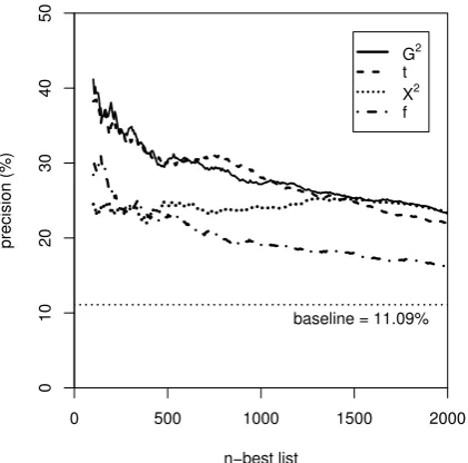
f ≥ 30 was applied, resulting in a candidate set of5 102 PP-verb pairs. The candidates were then ranked according to the scores assigned by four association measures: the log-likelihood ratio G2 (Dunning, 1993), Pearson’s chi-squared statisticX2
(Manning and Sch¨utze, 1999, 169–172), the t-score statistict(Church et al., 1991), and mere cooccur-rence frequency f.4 TPs were identified according to the definition of Krenn (2000). The graphs in Figure 1 show the precision achieved by these mea-sures, for nranging from 100 to 2 000 (lists with n < 100were omitted because the graphs become highly unstable for smalln). The baseline precision of11.09%corresponds to a random selection of n candidates.
0 500 1000 1500 2000
0
10
20
30
40
50
n−best list
precision (%)
baseline = 11.09% G2
t X2
f
Figure 1: Evaluation example: candidates for Ger-man PP-verb collocations are ranked by four differ-ent association measures.
From Figure 1, we can see thatG2 andtare the most useful ranking methods, t being marginally better forn≈800andG2forn≥1 500. Both
mea-sures are by far superior to frequency-based rank-ing. The evaluation results also confirm the argu-ment of Dunning (1993), who suggested G2 as a more robust alternative toX2. Such results cannot be taken at face value, though, as they may simply be due to chance. When two equally useful rank-ing methods are compared, method A might just happen to perform better in a particular experiment, with B taking the lead in a repetition of the
experi-experiment, the corpus was annotated with the partial parser YAC (Kermes, 2003).
4See Evert (2004) for detailed information about these
as-sociation measures, as well as many further alternatives.
ment under similar conditions. The causes of such random variation include the source material from which the candidates are extracted (what if a slightly different source had been used?), noise introduced by automatic pre-processing and extraction tools, and the uncertainty of human annotators manifested in varying degrees of inter-annotator agreement. Most researchers understand the necessity of test-ing whether their results are statistically significant, but it is fairly unclear which tests are appropriate. For instance, Krenn (2000) applies the standardχ2 -test to her comparative evaluation of collocation ex-traction methods. She is aware, though, that this test assumes independent samples and is hardly suit-able for different ranking methods applied to the same candidate set: Krenn and Evert (2001) sug-gest several alternative tests for related samples. A wide range of exact and asymptotic tests as well as computationally intensive randomisation tests (Yeh, 2000) are available and add to the confusion about an appropriate choice.
The aim of this paper is to formulate a statisti-cal model that interprets the evaluation of ranking methods as a random experiment. This model de-fines the degree to which evaluation results are af-fected by random variation, allowing us to derive appropriate significance tests. After formalising the evaluation procedure in Section 2, I recast the pro-cedure as a random experiment and make the under-lying assumptions explicit (Section 3.1). On the ba-sis of this model, I develop significance tests for the precision of a single ranking method (Section 3.2) and for the comparison of two ranking methods (Section 3.3). The paper concludes with an empiri-cal validation of the statistiempiri-cal model in Section 4.
2 A formal account of ranking methods
and their evaluation
In this section I present a formalisation of rankings and their evaluation, givingγ-acceptance sets a ge-ometrical interpretation that is essential for the for-mulation of a statistical model in Section 3.
The scores computed by a ranking method are based on certain features of the candidates. Each candidate can therefore be represented by its feature
vectorx∈Ω, whereΩis an abstract feature space. For all practical purposes,Ωcan be equated with a subset of the (possibly high-dimensional) real Eu-clidean spaceRm. The complete set of candidates corresponds to a discrete subsetC ⊆ Ωof the fea-ture space.5 A ranking method is represented by
5
a real-valued function g : Ω → R on the feature space, called a scoring function (SF). In the follow-ing, I assume that there are no candidates with equal scores, and hence no ties in the rankings.6
Theγ-acceptance set for a SFgcontains all can-didates x ∈ C with g(x) ≥ γ. In a geomet-rical interpretation, this condition is equivalent to x∈Ag(γ)⊆Ω, where
Ag(γ) :={x∈Ω |g(x)≥γ}
is called the γ-acceptance region of g. The γ -acceptance set ofgis then given by the intersection Ag(γ)∩C=:Cg(γ). The selection of ann-best list is based on theγ-acceptance regionAg(γg(n))for a suitably chosenn-best thresholdγg(n).7
As an example, consider the collocation extrac-tion task introduced in Secextrac-tion 1. The feature vec-tor x associated with a collocation candidate rep-resents the cooccurrence frequency information for this candidate: x = (O11, O12, O21, O22), where
Oij are the cell counts of a 2 × 2 contingency table (Evert, 2004). Therefore, we have a four-dimensional feature space Ω ⊆ R4, and each
as-sociation measure defines a SFg : Ω → R. The selection of collocation candidates is usually made in the form of ann-best list, but may also be based on a pre-defined thresholdγ.8
For an evaluation in terms of precision and re-call, the candidates in the set C are classified into
true positivesC+ and false positivesC−. The
pre-cision corresponding to an acceptance region A is then given by
ΠA:=|C+∩A|/|C∩A|, (1)
i.e. the proportion of TPs among the accepted candi-dates. The precision achieved by a SFgwith thresh-oldγ isΠCg(γ). Note that the numerator in Eq. (1)
reduces to n for an n-best list (i.e. γ = γg(n)), yielding then-best precisionΠg,n. Figure 1 shows graphs ofΠg,nfor 100 ≤ n ≤ 2 000, for the SFs g1=G2,g2=t,g3 =X2, andg4 =f.
can be enforced by adding a small amount of random jitter to the feature vectors of candidates.
6
Under very general conditions, random jittering (cf. Foot-note 5) ensures that no two candidates have equal scores. This procedure is (almost) equivalent to breaking ties in the rankings randomly.
7Since I assume that there are no ties in the rankings,γ
g(n)
can always be determined in such a way that the acceptance set contains exactlyncandidates.
8
For instance, Church et al. (1991) use a threshold ofγ = 1.65for the t-score measure corresponding to a nominal sig-nificance level ofα=.05. This threshold is obtained from the limiting distribution of thetstatistic.
3 Significance tests for evaluation results
3.1 Evaluation as a random experiment
When an evaluation experiment is repeated, the re-sults will not be exactly the same. There are many causes for such variation, including different source material used by the second experiment, changes in the tool settings, changes in the evaluation criteria, or the different intuitions of human annotators. Sta-tistical significance tests are designed to account for a small fraction of this variation that is due to ran-dom effects, assuming that all parameters that may have a systematic influence on the evaluation results are kept constant. Thus, they provide a lower limit for the variation that has to be expected in an actual repetition of the experiment. Only when results are significant can we expect them to be reproducible, but even then a second experiment may draw a dif-ferent picture.
In particular, the influence of qualitatively differ-ent source material or differdiffer-ent evaluation criteria can never be predicted by statistical means alone. In the example of the collocation extraction task, randomness is mainly introduced by the selection of a source corpus, e.g. the choice of one partic-ular newspaper rather than another. Disagreement between human annotators and uncertainty about the interpretation of annotation guidelines may also lead to an element of randomness in the evaluation. However, even significant results cannot be gener-alised to a different type of collocation (such as adjective-noun instead of PP-verb), different eval-uation criteria, a different domain or text type, or even a source corpus of different size, as the results of Krenn and Evert (2001) show.
A first step in the search for an appropriate sig-nificance test is to formulate a (plausible) model for random variation in the evaluation results. Be-cause of the inherent randomness, every repetition of an evaluation experiment under similar condi-tions will lead to different candidate sets C+ and
C−. Some elements will be entirely new candidates,
sometimes the same candidate appears with a ent feature vector (and thus represented by a differ-ent pointx ∈ Ω), and sometimes a candidate that was annotated as a TP in one experiment may be annotated as a FP in the next. In order to encapsu-late all three kinds of variation, let us assume that C+ andC−are randomly selected from a large set
of hypothetical possibilities (where each candidate corresponds to many different possibilities with dif-ferent feature vectors, some of which may be TPs and some FPs).
inA,FA := |C−∩A|, are thus random variables.
We do not know their precise distributions, but it is reasonable to assume that (i)TAandFAare always independent and (ii)TAandTB(as well asFAand FB) are independent for any two disjoint regionsA and B. Note that TA andTB cannot be indepen-dent forA∩B 6= ∅because they include the same number of TPs from the region A∩B. The total number of candidates in the regionAis also a ran-dom variableNA:=TA+FA, and the same follows for the precisionΠA, which can now be written as
ΠA=TA/NA.9
Following the standard approach, we may now assume that ΠA approximately follows a normal distribution with mean πA and variance σA2, i.e.
ΠA∼N(πA, σ2A). The meanπAcan be interpreted as the average precision of the acceptance region A(obtained by averaging over many repetitions of the evaluation experiment). However, there are two problems with this assumption. First, while ΠA is an unbiased estimator forπa, the variance σA2 can-not be estimated from a single experiment.10 Sec-ond,ΠAis a discrete variable because bothTAand NA are non-negative integers. When the number of candidatesNA is small (as in Section 3.3), ap-proximating the distribution ofΠAby a continuous normal distribution will not be valid.
It is reasonable to assume that the distribution of NAdoes not depend on the average precisionπA. In this case,NAis called an ancillary statistic and can be eliminated without loss of information by condi-tioning on its observed value (see Lehmann (1991, 542ff) for a formal definition of ancillary statistics and the merits of conditional inference). Instead of probabilitiesP(ΠA)we will now consider the con-ditional probabilities P(ΠA|NA). Because NA is fixed to the observed value, ΠA is proportional to TAand the conditional probabilities are equivalent to P(TA|NA). When we choose one of the NA candidates at random, the probability that it is a TP (averaged over many repetitions of the experiment)
9In the definition of the n-best precision Π
g,n, i.e. for
A =Cg(γg(n)), the number of candidates inAis constant:
NA =n. At first sight, this may seem to be inconsistent with
the interpretation ofNA as a random variable. However, one
has to keep in mind thatγg(n), which is determined from the
candidate setC, is itself a random variable. Consequently,Ais
not a fixed acceptance region and its variation counter-balances
that ofNA.
10Sometimes, cross-validation is used to estimate the
vari-ability of evaluation results. While this method is appropri-ate e.g. for machine learning and classification tasks, it is not useful for the evaluation of ranking methods. Since the cross-validation would have to be based on random samples from a single candidate set, it would not be able to tell us anything about random variation between different candidate sets.
should be equal to the average precisionπA. Conse-quently, P(TA|NA) should follow a binomial dis-tribution with success probabilityπA, i.e.
P(TA=k|NA) =
NA k
·(πA)k·(1−πA)NA−k (2)
for k = 0, . . . , NA. We can now make inferences about the average precision πAbased on this bino-mial distribution.11
As a second step in our search for an appropriate significance test, it is essential to understand exactly what question this test should address: What does it mean for an evaluation result (or result difference) to be significant? In fact, two different questions can be asked:
A: If we repeat an evaluation experiment under
the same conditions, to what extent will the ob-served precision values vary? This question is
addressed in Section 3.2.
B: If we repeat an evaluation experiment under
the same conditions, will method A again per-form better than method B? This question is
addressed in Section 3.3.
3.2 The stability of evaluation results
Question A can be rephrased in the following way:
How much does the observed precision value for an acceptance region A differ from the true aver-age precision πA? In other words, our goal here is to make inferences about πA, for a given SF g and threshold γ. From Eq. (2), we obtain a bino-mial confidence interval for the true valueπA, given the observed values ofTAandNA(Lehmann, 1991, 89ff). Using the customary 95% confidence level, πAshould be contained in the estimated interval in all but one out of twenty repetitions of the experi-ment. Binomial confidence intervals can easily be computed with standard software packages such as R (R Development Core Team, 2003). As an ex-ample, assume that an observed precision ofΠA=
40% is based onTA = 200TPs out ofNA = 500 accepted candidates. Precision graphs as those in Figure 1 display ΠAas a maximum-likelihood es-timate for πA, but its true value may range from
35.7%to44.4%(with 95% confidence).12
11
Note that some of the assumptions leading to Eq. (2) are far from self-evident. As an example, (2) tacitly assumes that the success probability is equal toπAregardless of the
particu-lar value ofNAon which the distribution is conditioned, which
need not be the case. Therefore, an empirical validation is nec-essary (see Section 4).
12This confidence interval was computed with the R
Figure 2 shows binomial confidence intervals for the association measuresG2 andX2 as shaded re-gions around the precision graphs. It is obvious that a repetition of the evaluation experiment may lead to quite different precision values, especially forn <1 000. In other words, there is a consider-able amount of uncertainty in the evaluation results for each individual measure. However, we can be confident that both ranking methods offer a substan-tial improvement over the baseline.
0 500 1000 1500 2000
0
10
20
30
40
50
n−best list
precision (%)
baseline = 11.09% G2
X2
Figure 2: Precision graphs for theG2 andX2 mea-sures with 95% confidence intervals.
For an evaluation based onn-best lists (as in the collocation extraction example), it has to be noted that the confidence intervals are estimates for the average precision πA of a fixed γ-acceptance re-gion (withγ =γg(n)computed from the observed candidate set). While this region contains exactly NA = ncandidates in the current evaluation, NA may be different fromnwhen the experiment is re-peated. Consequently,πAis not necessarily identi-cal to the average precision ofn-best lists.
3.3 The comparison of ranking methods
Question B can be rephrased in the following way:
Does the SFg1on average achieve higher precision than the SFg2? (This question is normally asked
wheng1performed better thang2in the evaluation.)
In other words, our goal is to test whetherπA> πB for given acceptance regionsAofg1andBofg2.
The confidence intervals obtained for two SF g1
and g2 will often overlap (cf. Figure 2, where the
confidence intervals of G2 and X2 overlap for all list sizes n), suggesting that there is no significant
difference between the two ranking methods. Both observed precision values are consistent with an av-erage precisionπA = πB in the region of overlap, so that the observed differences may be due to ran-dom variation in opposite directions. However, this conclusion is premature because the two rankings are not independent. Therefore, the observed pre-cision values of g1 andg2 will tend to vary in the
same direction, the degree of correlation being de-termined by the amount of overlap between the two rankings. Given acceptance regions A := Ag1(γ1)
andB :=Ag2(γ2), both SF make the same decision
for any candidates in the intersection A∩B (both SF accept) and in the “complement” Ω\(A∪B)
(both SF reject). Therefore, the performance of g1
andg2 can only differ in the regionsD1 := A\B
(g1 accepts, butg2 rejects) andB\A (vice versa).
Correspondingly, the counts TAandTB are corre-lated because they include the same number of TPs from the regionA∩B(namely, the setC+∩A∩B),
Indisputably, g1 is a better ranking method than
g2 iffπD1 > πD2 and vice versa.
13 Our goal is thus
to test the null hypothesisH0 :πD1 = πD2 on the
basis of the binomial distributions P(TD1|ND1)
and P(TD2|ND2). I assume that these
distribu-tions are independent because D1 ∩D2 = ∅ (cf.
Section 3.1). The number of candidates in the difference regions, ND1 and ND2, may be small,
especially for acceptance regions with large over-lap (this was one of the reasons for using condi-tional inference rather than a normal approximation in Section 3.1). Therefore, it is advisable to use Fisher’s exact test (Agresti, 1990, 60–66) instead of an asymptotic test that relies on large-sample ap-proximations. The data for Fisher’s test consist of a2×2contingency table with columns(TD1, FD1)
and(TD2, FD2). Note that a two-sided test is called
for because there is no a priori reason to assume that g1 is better thang2 (or vice versa). Although
the implementation of a two-sided Fisher’s test is not trivial, it is available in software packages such as R.
Figure 3 shows the same precision graphs as Figure 2. Significant differences between the G2 and X2 measures according to Fisher’s test (at a 95% confidence level) are marked by grey triangles.
13
Note thatπD1 > πD2 does not necessarily entailπA >
πB ifNA andNB are vastly different andπA∩B πDi. In
this case, the winner will always be the SF that accepts the smaller number of candidates (because the additional candi-dates only serve to lower the precision achieved inA∩B). This example shows that it is “unfair” to compare acceptance sets of (substantially) different sizes just in terms of their over-all precision. Evaluation should therefore either be based on
Contrary to what the confidence intervals in Fig-ure 2 suggested, the observed differences turn out to be significant for alln-best lists up ton= 1 250
(marked by a thin vertical line).
0 500 1000 1500 2000
0
10
20
30
40
50
n−best list
precision (%)
baseline = 11.09% G2
X2
Figure 3: Significant differences between the G2 andX2measures at 95% confidence level.
4 Empirical validation
In order to validate the statistical model and the sig-nificance tests proposed in Section 3, it is neces-sary to simulate the repetition of an evaluation ex-periment. Following the arguments of Section 3.1, the conditions should be the same for all repetitions so that the amount of purely random variation can be measured. To achieve this, I divided the Frank-furter Rundschau Corpus into 80 contiguous, non-overlapping parts, each one containing approx. 500k words. Candidates for PP-verb collocations were extracted as described in Section 1, with a frequency threshold of f ≥ 4. The 80 samples of candidate sets were ranked using the association measuresG2, X2 and t as scoring functions, and true positives were manually identified according to the criteria of (Krenn, 2000).14 The true average precisionπA of an acceptance setAwas estimated by averaging over all 80 samples.
Both the confidence intervals of Section 3.2 and the significance tests of Section 3.3 are based on the assumption thatP(TA|NA)follows a binomial distribution as given by Eq. (2). Unfortunately, it
14
I would like to thank Brigitte Krenn for making her annota-tion database of PP-verb collocaannota-tions (Krenn, 2000) available, and for the manual annotation of1 913candidates that were not covered by the existing database.
is impossible to test the conditional distribution di-rectly, which would require thatNAis the same for all samples. Therefore, I use the following approach based on the unconditional distributionP(ΠA). If NAis sufficiently large,P(ΠA|NA)can be approx-imated by a normal distribution with meanµ=πA and varianceσ2 =πA(1−πA)/NA(from Eq. (2)). Since µ does not depend onNA and the standard deviationσ is proportional to(NA)−1/2, it is valid to make the approximation
P(ΠA|NA)≈P(ΠA) (3)
as long asNAis relatively stable. Eq. (3) allows us to pool the data from all samples, predicting that
P(ΠA)∼N(µ, σ2) (4)
withµ = πA andσ2 = πA(1−πA)/N. Here,N stands for the average number of TPs inA.
These predictions were tested for the measures g1 = G2 andg2 = t, with cutoff thresholdsγ1 = 32.5andγ2 = 2.09(chosen so thatN = 100
candi-dates are accepted on average). Figure 4 compares the empirical distribution ofΠAwith the expected distribution according to Eq. (4). These histograms show that the theoretical model agrees quite well with the empirical results, although there is a lit-tle more variation than expected.15 The empirical standard deviation is between20%and40%larger than expected, withs= 0.057vs.σ= 0.044forG2 ands= 0.066vs.σ = 0.047fort. These findings suggest that the model proposed in Section 3.1 may indeed represent a lower bound on the true amount of random variation.
Further evidence for this conclusion comes from a validation of the confidence intervals defined in Section 3.2. For a 95% confidence interval, the true proportionπAshould fall within the confidence in-terval in all but 4 of the 80 samples. ForG2 (with γ = 32.5) andX2 (withγ = 239.0),πAwas out-side the confidence interval in 9 cases each (three of them very close to the boundary), while the con-fidence interval fort(withγ = 2.09) failed in 12 cases, which is significantly more than can be ex-plained by chance (p < .001, binomial test).
5 Conclusion
In the past, various statistical tests have been used to assess the significance of results obtained in the evaluation of ranking methods. There is much con-fusion about their validity, though, mainly due to
15
Histogram for G2
precision
number of samples
0.0 0.1 0.2 0.3 0.4 0.5 0.6
0
5
10
15
20 observed
expected
Histogram for t
precision
number of samples
0.0 0.1 0.2 0.3 0.4 0.5 0.6
0
5
10
15
20
observed expected
Figure 4: Distribution of the observed precisionΠAforγ-acceptance regions of the association measures G2(left panel) andt(right panel). The solid lines indicate the expected distribution according to Eq. (2).
the fact that assumptions behind the application of a test are seldom made explicit. This paper is an attempt to remedy the situation by interpret-ing the evaluation procedure as a random experi-ment. The model assumptions, motivated by intu-itive arguments, are stated explicitly and are open for discussion. Empirical validation on a colloca-tion extraccolloca-tion task has confirmed the usefulness of the model, indicating that it represents a lower bound on the variability of evaluation results. On the basis of this model, I have developed appro-priate significance tests for the evaluation of rank-ing methods. These tests are implemented in the UCS toolkit, which was used to produce the graphs in this paper and can be downloaded fromhttp: //www.collocations.de/.
References
Alan Agresti. 1990. Categorical Data Analysis. John Wiley & Sons, New York.
Kenneth Church, William Gale, Patrick Hanks, and Donald Hindle. 1991. Using statistics in lexical analysis. In Lexical Acquisition: Using On-line
Resources to Build a Lexicon, pages 115–164.
Lawrence Erlbaum.
Ted Dunning. 1993. Accurate methods for the statistics of surprise and coincidence.
Computa-tional Linguistics, 19(1):61–74.
Stefan Evert and Brigitte Krenn. 2001. Methods for the qualitative evaluation of lexical associa-tion measures. In Proceedings of the 39th Annual
Meeting of the Association for Computational Linguistics, pages 188–195, Toulouse, France.
Stefan Evert. 2004. An on-line
reposi-tory of association measures. http: //www.collocations.de/AM/.
Hannah Kermes. 2003. Off-line (and On-line) Text
Analysis for Computational Lexicography. Ph.D.
thesis, IMS, University of Stuttgart. Arbeitspa-piere des Instituts f¨ur Maschinelle Sprachverar-beitung (AIMS), volume 9, number 3.
Brigitte Krenn and Stefan Evert. 2001. Can we do better than frequency? a case study on ex-tracting pp-verb collocations. In Proceedings of
the ACL Workshop on Collocations, pages 39–46,
Toulouse, France, July.
Brigitte Krenn. 2000. The Usual Suspects:
Data-Oriented Models for the Identification and Rep-resentation of Lexical Collocations., volume 7 of Saarbr¨ucken Dissertations in Computational Lin-guistics and Language Technology. DFKI &
Uni-versit¨at des Saarlandes, Saarbr¨ucken, Germany. E. L. Lehmann. 1991. Testing Statistical
Hypothe-ses. Wadsworth, 2nd edition.
Christopher D. Manning and Hinrich Sch¨utze. 1999. Foundations of Statistical Natural
Lan-guage Processing. MIT Press, Cambridge, MA.
R Development Core Team, 2003. R: A language
and environment for statistical computing. R
Foundation for Statistical Computing, Vienna, Austria. ISBN 3-900051-00-3. See alsohttp: //www.r-project.org/.
Alexander Yeh. 2000. More accurate tests for the statistical significance of result differences. In
Proceedings of the 18th International Conference on Computational Linguistics (COLING 2000),