Introduction to the MT Plateau
We believe it is fair to say that the field of machine translation has been on a plateau for at least the past decade.2 Traditional, hand-built MT systems held up very well in the ARPA MT evaluation (White and O'Connell 1994). These systems are relatively expensive to build and generally require a trained staff working for several years to produce a mature system. This is the current commercial state of the art: hand-building specialized lexicons and translation rules. A completely different type of system was competitive in this evaluation, namely, the purely statistical CANDIDE system built at IBM. It was generally felt that this system had also reached a plateau in that more data and more training was not likely to improve the quality of the output.
Low Density Machine Translation
However, in the case of "Low Density Machine Translation" (see Nirenburg and Raskin 1998, Jones and Havrilla 1998) commercial market forces are not likely to provide significant incentives for machine translation systems for Low Density (Non-Major) languages any time soon. Two noteworthy efforts to break past the data and labor bottlenecks for high-quality machine translation development are the following. The NSF Summer Workshop on
2 A sensible, plateau-friendly strategy may be to
accumulate translation memory to improve both the long-term efficiency of human translators and the quality of machine translation systems. If we imagine that the plateau is really a kind of logarithmic function tending ever upwards, we need only be patient.
Statistical Machine Translation held at Johns Hopkins University summer 1999 developed a public-domain version intended as a platform for further development of a CANDIDE-style MT system. Part of the goal here is to improve the translation by adding levels of linguistic analysis beyond the word N-gram. An effort addressing the labor bottleneck is the Expedition Project at New Mexico State University where a preliminary elicitation environment for a computational field linguistics system has been developed (the Boas interface; see Nirenburg and Raskin 1998)
A Scoring Function for MT quality
Our contribution toward working beyond this plateau is to look for a way to define a scoring function for the quality of the English output such that we can use it to machine-learn a good translation grammar. The novelty of our idea for this function is that we do not have to define the internals of it ourselves per se. We are able to define a successful function for two reasons. First, there is a growing body of software worldwide that has been designed to consume English; all we need is for each piece of software to provide a metric as to how English-like its input is. Second, we can tell whether the software had trouble with the input, either by system-internal diagnosis or by diagnosing the software's output. A good illustration is the facility in current word-processing software to put red squiggly lines underneath text it thinks should be revised. We know from experience that this feature is often only annoying. Nevertheless, imagine that it is correct some percentage of the time, and that each piece of software we use for this purpose is correct some percentage of the time. Our strategy is to
Toward a Scoring Function for Quality-Driven Machine Translation
Abstract
We describe how we constructed an automatic scoring function for machine translation quality; this function makes use of arbitrarily many pieces of natural language processing software that has been designed to process English language text. By machine-learning values of functions available inside the software and by constructing functions that yield values based upon the software output, we are able to achieve preliminary, positive results in machine-learning the difference between human-produced English and machine-translation English. We suggest how the scoring function may be used for MT system development.
Douglas A. Jones 1 Department of Defense 9800 Savage Road, Suite 6514 Fort Meade, MD 20755-6514
Gregory M. Rusk RABA Technologies
10500 Little Patuxent Parkway Columbia, MD 21044
extract or create numeric values from each piece of software that corresponds to the degree to which the software was happy with the input. That array of numbers is the heart of our scoring function for Englishness -- we are calling these numeric values "indicators" of Englishness. We then use that array of indicators to drive the machine translation development. In this paper we will report on how we have constructed a prototype of this function; in separate work we discuss how to insert this function into a machine-learning regimen designed to maximize the overall quality of the machine translation output.
A Reverse Turing Test
People can generally tell the difference between human-produced English and machine translation English, assuming all the obvious constraints such as that the reader and writer have command of the language. Whether or not a machine can tell the difference depends of course, on how good the MT system is. Can we get a machine to tell the difference? Of course it depends on how good the MT system is: if it were perfect, neither we nor the machines ought to be able to distinguish them. MT quality being what it is, that is not a problem for us now. An essential first step toward QDMT is what we are calling a "Reverse Turing Test". In the ordinary Turing Test, we want to fool a person into thinking the machine is a person. Here, we are turning that on its head. We want to define a function that can tell the difference between English that a human being has produced versus English that the machine has produced.3 To construct the test, we use a bilingual parallel aligned corpus: we take the foreign language side and send that through the MT system; then we see if we can define a scoring function that can distinguish the two versions (original English and MT English). With our current indicators and corpus, we can machine-learn a function that behaves as follows: if you hand it a human sentence, it correctly classifies it as human 74% of the time. If you hand it a machine sentence, it correctly classifies it as a machine sentence 57% of the time. In the remainder of the paper, we will step through the details of the experiment; we will also discuss why we
3Obviously the end goal here is to fail this Reverse
Turing Test for a "perfect" machine translation system. We are very far away from this, but we would like to use this function to drive the process toward that eventual and fortunate failure.
neither expect nor require 100% accuracy for this function. Our boundary tests behave as expected and are shown in the final section --we use the same test to distinguish bet--ween English and (a) English word salad, (b) English alphabet soup, (c) Japanese, and (d) the identity case of more human-produced English.
Case Study: Japanese-English
In this paper, we report on results using a small corpus of 2,340 sentences drawn from the Kenkyusha New Japanese-English Dictionary. It was important in this particular experiment to use a very clean corpus (perfectly aligned and minimally formatted). This case study is situated in a broader context: we have conducted exploratory experiments on samples from several corpora, for example the ARPA MT Evaluation corpus, samples from European Corpus Initiative Data corpus (ECI-1) and others. Since we found that the scoring function was quite sensitive to formatting problems (for example, the presence of tables and sentence segmentation errors cause problems) we are examining a small corpus that is free from these issues. The sentences are on average relatively short (7.0 words per sentence; 37.6 characters/sentence), this makes our task both easier and harder. It is easier because we have overcome the formatting problems. It is harder because the MT system is able to perform much better on the shorter, cleaner sentences than it was on longer sentences with formatting problems. Since the output is better, it is more difficult to define a function that can tell the difference between the original English and the machine translation English. On balance, this corpus is a good one to illustrate our technique.
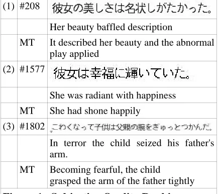
(1) #208
Her beauty baffled description
MT It described her beauty and the abnormal play applied
(2) #1577
She was radiant with happiness
MT She had shone happily
(3) #1802
In terror the child seized his father's arm.
MT Becoming fearful, the child
grasped the arm of the father tightly
Figure 1 shows a range of output quality. (1) is the worst -- it is obviously MT output. For us this output is only partially intelligible. (2) is not so bad, but it is still not perfect English. But (3)is nearly perfect. We want to design a system that can tell the difference. We will now walk through our suite of indicators; the goal is to get the machine to see what we see in terms of quality.
Suite of Indicators
We have defined a suite of functions that operate at various levels of linguistic analysis: syntactic, semantic, and phonological (orthographic). For each of these levels, we have integrated at least one tool for which we construct an indicator function. The task is to use these indicators to generate an array of values which we can use to capture the subjective quality we see when we read the sentences. We will step through these indicator functions one by one. In some cases, in order to get numbers, we take what amounts to debugging information from the tool (many of the tools have very nice API's that give access to a variety of information about how it processed input). In other cases, we define a function that yields an output based on the output of the tool (for example, we defined a function that indicated the degree to which a parse tree was balanced; it turned out that a balanced tree was a negative indicator of Englishness, probably because English is right-branching).
Syntactic Indicators
Two sources of local syntactic information are (a) parse trees and (b) N-grams. Within the parsers, we looked at internal processing information as well as output structures. For example, we measured the probability of a parse and number of edges in the parse from the Collins parser. The Apple Pie Parser provided various weights which we used. The Appendix lists all of the indicator functions that we used.
N-Gram Language Model (Cross-Perplexity)
An easy number to calculate is the cross-perplexity of a given text, as calculated using an N-gram language model.4
4 We used the Cambridge/CMU language modeling
toolkit, trained on the Wall Street Journal (4/1990 through 3/1992), (lm parameters: n=4, Good-Turing smoothing)
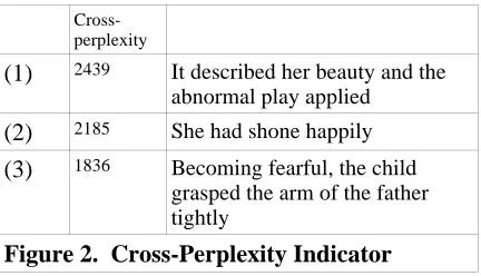
Cross-perplexity
(1) 2439 It described her beauty and the
abnormal play applied
(2) 2185 She had shone happily
(3) 1836 Becoming fearful, the child
grasped the arm of the father tightly
Figure 2. Cross-Perplexity Indicator
Notice that the subjective order is mirrored by the cross-perplexity scores in Figure 2.
Collins Parser
The task here is to write functions that process the parse trees and return a number. We have experimented with more elaborate functions that indicate how balanced the parse tree is and less complicated functions such as the level of embedding, number of parentheses, and so on. Interestingly, the number of parentheses in the parse was a helpful indicator in conjunction with other indicators.
Indicators of Semantic Cohesiveness
For the semantic indicators, we want some indication as to how much the words in a text are related to each other by virtue of their meaning. Which words belong together, regardless of exactly how they are used in the sentence? Two resources we have begun to integrate for this purpose are WordNet and the Trigger Toolkit (measuring mutual information). The overall experimental design is roughly the same in both cases. Our method was to remove stop words, lemmatize the text, and then take a measurement of pairwise semantic cohesiveness of the lemmatized words5. For WordNet, we are counting how many ways two words are related by the hyponymy relation (future indicators will be more sophisticated). For the Trigger Toolkit, we weighted the connections (by mutual information).Orthographic
We had two motivations for an orthographic level: one was methodological (we wanted to look at each of the traditional levels of linguistic analysis). The other was driven by our experience in looking at the MT output. Some MT systems leave untranslated words
5The following parameters were used to build and
alone, or transliterate them, or insert a dummy symbol, such as "X". These clues were adequate to give us appropriate hints as to whether the text was produced by human or by machine. But some of our tools missed these clues because of how they were designed. Robust parsers often treat unknown words as nouns; so if we get an untranslated term or an "X", the parser simply treats it as a noun. Five X's in a row might be a noun phrase followed by a verb.6Smoothed N-gram models of words
usually treat any string of letters as a possible word.
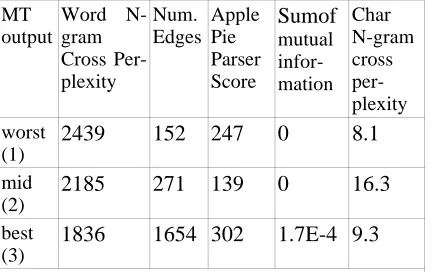
1836 1654 302 1.7E-4 9.3 Figure 3. Subjective and Objective Rankings Because the parsers and N-gram models were designed to be very robust, they are not necessarily sensitive to these obvious clues. In order to get at these hints, we built a character-based N-gram model of English. Although these indicators were not very informative on their own for distinguishing human from machine English, they boosted performance in conjunction with the syntactic and semantic indicators.
Combined Indicators
Let's come back to the three sentences from Figure 1: we want to capture our subjective ranking of the sentences with appropriate indicator values. In other words, we want the machine to be able to see differences which a human might see.
For these three examples, some scores correlate well with our subjective ranking of Englishness (e.g. cross-perplexity, Edges). However, the other scores on their own only partially correlate. The expectation is that an indicator on its own will not be sufficient to score the Englishness. It is the combined effect of all indicators which ultimately decides the
6We found that we could often guess the "default"
behavior that a parser used and we have begun to design indicators that can tell when a parser has defaulted to these.
Englishness. Now we have enough raw data to begin machine-learning a way to distinguish these kinds of sentences.
Simple Machine Learning Regimen
We have started out with very simple memory-based machine learning techniques. Since we are defining a range of functions, we wanted to keep things relatively simple for debugging and didactic purposes.KNN
One of the simplest methods we can use for classification is to collect values of the N indicators for a set of training cases and for the test cases, to find the K nearest training cases (using Euclidean distance in N-dimensional space). For K, we used 5 for our general experiments (but see below for some variations). For a concrete example in two dimensions, imagine that we use the cross-perplexity of an N-gram language model for the Y-axis and the probability of a parse from the Collins parser for the X-axis. Human sentences tended to have better (lower) cross-perplexity numbers and better (higher) parse probabilities. If the 5 nearest neighbors to a data point were (h,h,h,h,m) four human sentences and one machine our KNN function guesses that it is a human sentence.
Figure 4 lists some of the parameters we used for KNN. The values for cross perplexity ranged from around 100 to 10,000 and the Collins parse probability (log) ranged from around -1000 to 0. These values were normalized to range from 0-1.
All columns were scaled between 0 and 1. - Value for K in KNN was set to 5. - Value for L in KNN was set to 0 (L is the minimum number of positive neighbors required for a confident classification i.e. L=5 means all neighbors must be of one class)
- Distance calculation is Euclidean - We used 10-fold cross-validation and calculated the average classification accuracy for the overall score.
Figure 4. KNN Parameters
machine (the remaining 44% were not classified). By setting L to 5 (eliminating guessing) these numbers dropped to 18% and 2% respectively. When we varied K (for example, trying K of 101) we found that we can increase the performance of the human classifier to nearly 90%. Performance of KNN tended to top out at around 74% with the parameters in Figure 4.
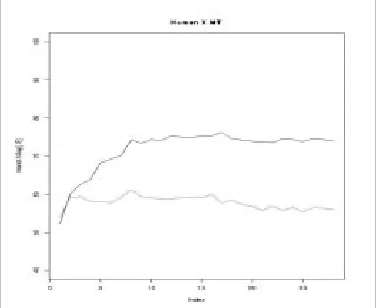
Indicator Monotonicity
There is no guarantee that classification will perform better with more dimensions in KNN. However, we found that we generally got a monotonically increasing performance in classification when we added indicator functions. A helpful analogy might be to consider the blind men and the elephant. In our case, "English" is the elephant, and each of our indicator functions is one blind man grasping at the elephant. One is grasping at semantics, one at syntax, and so on. Figure 5 shows how classification improves with more indicators (the back of the elephant, so to speak).
Benchmarks
To calibrate the indicator functions we have used to classify text into human- or machine-produced, we tested our method with some boundary cases, shown in Figure 6. The most extreme case was to learn the difference
between Japanese text (in native character encoding) and English.
Truth is:
human machine
Machine Guesses:
Japanese 99.6 99.6
Alphabet Soup 99.4 99.2
Word Salad 95.4 91.1
MT Output 74.0 56.1
Identity Case 52.3 49.4
Figure 6. Baselines
In other words, we have come up with a very computationally expensive method for Language Identification. Next less extreme was what we called "Alphabet Soup"; we took English sentences from the English side of the Kenkyusha corpus: for each alphabetic character, we substituted a randomly-selected alphabetic character, preserving case and punctuation.7 For "Word Salad", we took the English sentences from the Kenkyusha corpus and scrambled their order. MT Output is the case we discussed in detail above. The Identity Case is to divide the English sentences from the corpus into two piles and then try to tell them apart. As Figure 6 shows, the pathological baseline cases all work out very well: our machine can almost always tell that Japanese, Alphabet Soup, and Word Salad are not English. Nor can it distinguish between two arbitrarily divided piles of human English.
Other Classification Algorithms
We have performed some initial experiments with Support Vector Machines (SVM) as a classification method. SVM attempts to divide up an n-dimensional space using a set of support vectors defining a hyperplane. The basic approach of the SVM algorithm is different from KNN in that it actually deduces a classification model from the training data. KNN is a memory-based learning algorithm wherein the model is essentially a replica of the training examples.The initial trials using SVM are yielding classification accuracies of correctly classifying 83% of the human sentences and 64% of the machine sentences (single
7We found that it was often easy to crash some
of the software when we fed it arbitrary binary data, so we used "Alphabet Soup" instead of arbitrary binary data.
random sample of 10% withheld -- no n-fold cross-validation). These accuracies represent improvements of 11% for human test sentences and 14% for the machine test sentences. Further tests on this and other classification methods will be investigated to maximize performance in terms of accuracy and execution time.
Next Steps
There are two general areas we are continuing to work on: (a) to increase the scope and reliability of our indicators and (b) to insert the scoring function into a machine-learning regimen for producing translation grammars. In the first area, we have begun to explore the degree to which we might recapitulate the ARPA MT Evaluation. The data from these evaluations are freely available.8 Of course if all we did was recapitulate the data in some non-explanatory way, we would be doing something analogous to using the Chicago Bears to predict the stock market. The real work here is to map the objective scoring function numbers back to reliable subjective evaluation of the machine-produced texts. A crucial task for us here is to get a deeper understanding of how each of the pieces of software behaves with various types of input text. We are currently at a quite preliminary stage in terms of the number of indicators we are using and the degree to which each is fine-tuned to our purpose. For machine-learning a translation grammar, we have begun to explore using our scoring function to drive the construction of a prototype Low Density machine translation grammar compatible with a previous system built by hand. We have found that the scoring function is sensitive to the word order difference between the target English translation and the glosses for the source language. We would like to re-create a compatible knowledge base of the English half of the translation grammar using only the glosses as input. Such a technique would reduce the labor requirements in constructing a translation knowledge base.
Reverse
Turing
Scores
for
Machine
Learning Grammars
To illustrate how we can use the Reverse Turing scores to machine learn a grammar, let us consider a simple case of learning lexical features for a unification-based phrase structure grammar of the sort discussed in Jones &
8From ursula.georgetown.edu/mt_web.
Havrilla 1998. The working assumption there is that an adequate translation grammar can be created that conforms to the constraint that the only reordering that is allowed is the permutation of nodes in a binary-branching tree (as in Wu 1995, among others). How might we learn that postpositions and verbs generally trigger inversion? Consider the following example as shown in Figure 7 from Jones & Havrilla 1998; let us use +T to indicate that the lexical item triggers inversion; -T means that it does not. Let the initial state of the lexicon mark all lexical items as "-T".
S Shobhaa kamre-men baiThii hai
POS N N O V V
F -T -T +T +T +T
Shobha the_room-in sitting is
Figure 7. Shobha is sitting in the room.
Our machine learning process marks lexical items as "+T" when the Reverse Turing classification score for the bilingual corpus improves.
Conclusion
We are capitalizing on two historical accidents: (1) that English is a major world language and (2) that we want to translate into English. In addition to a variety of modern, standard NLP techniques and ideas, we have drawn from two unlikely sources of intellectual capital: (1) philosophy of language and (2) the current ubiquity of language engineering software. What we have taken from (1) is that we have assumed that there is such a thing as "English". That might not seem like much of an assumption, but we are treading near some very thorny problems in the philosophy of language. We can no more point to English than we can point to the perfect triangle. And like the blind men grasping at the elephant, how we characterize it depends on how we are exploring it. What is important is the helpful aggregate of numeric values that we use for the scoring. What does this mean for machine translation? We want to "Begin with the End in Mind"; in other words, we want the machine translation system to create output that scores well on our indicators of Englishness. The rest would be details, so to speak.
Acknowledgments
Appendix
List of current Indicators
1. Word N-Gram (CMU/Cambridge Language Tk) 2. Number of edges in parse (Collins Parser) 3. Log probability (Collins Parser) 4. Execution time (Collins Parser) 5. Paren count (Collins Parser)
6. Mean leaf node size of parse tree (Collins Parser) 7. Mean NN sequence length (Collins Parser) 8. Overall score (Apple Pie Parser)
9. Word level score (Apple Pie Parser) 10. Node count (Apple Pie Parser) 11. User execution time (Apple Pie Parser) 12. CD node count (Apple Pie Parser)
13. Mean CD sequence length (Apple Pie Parser)
14. Mean leading spaces in outline tree (from Collins Parse) 15. Tree balance ratio (from Collins Parse)
16. Tree depth (from Collins Parse)
17. Average minimum hypernym path length in WordNet 18. Average number hypernym paths in WordNet 19. Path found ratio in WordNet
20. Percent words with sense in WordNet 21. Sum of count of relations (Trigger Toolkit) 22. Mean of count of relations (Trigger Toolkit) 23. Sum of mutual information (Trigger Toolkit) 24. Mean of mutual information (Trigger Toolkit) 25. Pairs with mutual information (Trigger Toolkit)
26. Weighted pair sum of mutual information (Trigger Toolkit) 27. Number of target paired words (Trigger Toolkit
27. . N-Gram Cross-perplexity (Cambridge/CMU Lang Tk.)
Tools
TiMBL: Tilburg Memory Based Learner 2.0. ILK Research Group. http://ilk.kub.nl/software.html. PCKIMMO 2.0. Summer Institute of Linguistics. MXTERMINATOR. Adwait Ratnaparkhi. WEKA 3.0. University of Waikato.
ftp://ftp.cs.waikato.ac.nz/pub/ml/weka-3-0.jar Collins Parser 98.
Brill Tagger 1.14
R Statistical Package 0.65.0. http://cran.r-project.org/
Apple Pie Parser 5.8. New York University. http://cs.nyu.edu/cs/projects/proteus/app WordNet 1.6. ftp://ftp.cogsci.princeton.edu/~wn/ Trigger Toolkit 1.0. CMU.
http://www.cs.cmu.edu/~aberger/software.
References
Afifi, A.A., Virginia Clark. 1996. Computer-Aided Multivariate Analysis, 3rd ed.. New York, NY: Chapman and Hall.
Brill, Eric. 1995. Transformation-Based Error-Driven Learning and Natural Language Processing: A Case Study in Part Of Speech Tagging. (ACL).
Chambers, John M., William S. Cleveland, Beat Kleiner, and Paul A. Tukey. 1983. Graphical Methods for Data Analysis. Boston, MA: Duxbury Press.
Clarkson, Philip, Ronald Rosenfeld. 1997. Statistical Language Modeling Using the CMU-Cambridge Toolkit. Eurospeech97. Rhodes, Greece
Collins, Michael. 1997. Three Generative, Lexicalised Models for Statistical Parsing. Proceedings of the 35th Annual Meeting of the ACL/EACL), Madrid.
Daelemans, Walter, Jakub Zavrel and Ko van der Sloot. 1998. TiMBL: Tilburg Memory Based Learner, version 2.0, Reference Guide. Available from http://ilk.kub.nl/software.html.
Everitt, Brian S. and Graham Dunn. 1992. Applied Multivariate Data Analysis. New York, NY: Oxford University Press.
Fellbaum, Christiane (ed.). 1998. WordNet: An Electronic Lexical Database. Cambridge, MA: The MIT Press.
Flury, Bernhard and Hans Riedwyl. 1988. Multivariate Statistics. New York, NY: Chapman and Hall.
Hornik, Kurt. 1999. "The R FAQ". Available at http://www.ci.tuwien.ac.at/~hornik/R/.
Jones, Doug and Rick Havrilla. 1998. Twisted Pair Grammar: Support for Rapid Development of Machine Translation for Low Density Languages. AMTA-98. Langhorn, PA.
Knight, Kevin, Ishwar Chandler, Matthew Haines, Vasileios, Hatzivassigloglou, Eduard Hovy, Masayo Ida, Steve Luk, Richard, Whitney, and Kenji Yamada. 1994. Integrating Knowledge Bases and Statistics in MT (AMTA-94)
Manning, Christopher D. and Hinrich Schutze. 1999. Foundations of Statistical Natural Language Processing. Cambridge, MA: The MIT Press. Masuda, Koh (ed). 1974. Kenkyusha's New
Japanese-English Dictionary, 4th Ed. Tokyo: Kenkyusha.
Michalski, Ryszard S., Ivan Bratko, and Miroslav Kubat (eds.). 1998. Machine Learning and Data Mining. John Wiley & Son.
Mitchell, Tom M. 1997. Machine Learning. Boston, MA: McGraw-Hill.
Nirenburg, S. and V. Raskin. 1998. Universal Grammar and Lexis for Quick Ramp-Up of MT Systems. Proceedings of ACL/COLING `98. Montréal: University of Montreal (in press). Reynar, Jeffrey C. and Adwait Ratnaparkhi. 1997. A
Maximum Entropy Approach to Identifying Sentence Boundaries. ANLP-97. Washington, D.C.
Rosenfeld, Ronald. 1996. A Maximum Entropy Approach to Adaptive Statistical Language Modeling. Computer, Speech and Language. Witten, Ian H. and Eibe Frank. 1999. Data Mining:
Practical Machine Learning Tools and Techniques with Java Implementations. Morgan Kaufmann. White, J. and T.A. O'Connell. 1994. The ARPA MT
Evaluation Methodologies: Evolution, Lessons, and Future Approaches. Proceedings of AMTA-94