Proceedings of the 27th International Conference on Computational Linguistics, pages 1360–1371 1360
Local String Transduction as Sequence Labeling
Joana Ribeiro† Shashi Narayan† Shay B. Cohen† Xavier Carreras‡ †School of Informatics, University of Edinburgh, 10 Crichton Street, Edinburgh EH8 9AB, UK
‡dMetrics, Brooklyn, NY 11211, USA
[email protected] [email protected] [email protected] [email protected]
Abstract
We show that the general problem of string transduction can be reduced to the problem of sequence labeling. While character deletions and insertions are allowed in string transduction, they do not exist in sequence labeling. We show how to overcome this difference. Our approach can be used with any sequence labeling algorithm and it works best for problems in which string transduction imposes a strong notion of locality (no long range dependencies). We experiment with spelling correction for social media, OCR correction, and morphological inflection, and we see that it behaves better than seq2seq models and yields state-of-the-art results in several cases.
1 Introduction
String transduction (mapping one string to another) is an essential ingredient in the natural language processing (NLP) toolkit that helps solve problems ranging from morphological inflection (Dreyer et al., 2008) and lemmatization to spelling correction (Cotterell et al., 2014), text normalization (Porta and Sancho, 2013) and machine translation (Kumar et al., 2006).
Finite-state technology is often used with string transduction (Allauzen et al., 2007), especially when there is a strong notion of locality in the transduction problem, i.e., when there are no long range dependencies between the predicted characters. More recently, neural network methods have become more common for such problems using the seq2seq models that were introduced for machine translation (Bahdanau et al., 2015).
Similarly, sequence labeling algorithms have been the mainstay for an array of problems in NLP, including part-of-speech tagging, named entity recognition and semantic role labeling. Various models have been proposed to do sequence labeling, including conditional random fields, hidden Markov models and neural networks.
String transduction and sequence labeling are often treated as two separate entities, and indeed, usually give treatment to different problems in NLP. We claim and show that there is a great similarity between them, and that one can be reduced to the other.
Sequence labeling is often associated with a set of problems in which the set of labels is small compared to the vocabulary. Still, this labeling essentially associates each symbol (usually a word) in a sequence (usually a sentence) with a label. As such, it can be seen as a specific case of string transduction that imposes a one-to-one correspondence between input and output symbols. This is the easier side of the reduction between sequence labeling and string transduction, and it has been exploited in the deep learning literature with seq2seq models.
In this paper, we come to address the reduction in the reverse direction – i.e. we show how to frame string transduction as sequence labeling. We do this by decomposing the transduction process into two parts: first, we induce an alignment between the characters of the input and output strings and then we use a sequence labeling model to predict the final output of the string.
The main difficulty here is not in the size of the vocabulary compared to the label set, but the fact that string transduction can yield to arbitrary output string length compared to the input string. In machine
translation, for example, a classic example of string transduction, the sentence in the target language can be shorter, longer, and contain a significant amount of re-ordering. Indeed, re-ordering is a challenge with string transduction. A sequence labeling model usually maintains higher order of monotonicity (such as with Markovian models), while for general string transduction problems, one needs models such as encoder-decoders or grammatical models. Such expressive models, on the other hand, arenota good fit for string transduction problems with a strong notion of locality, as they are too complex and lead to weaker generalization power for such problems (Rastogi et al., 2016). We show this weakness in our experiments with seq2seq models supporting similar conclusions in previous work such as by Schnober et al. (2016). Our experiments show that even when seq2seq models are incorporated with hard monotonic attention (Aharoni and Goldberg, 2017), our reduction to sequence labeling outperforms such models on certain problems with a strong notion of locality.
Our approach to reduce string transduction to sequence labeling relies on a simple observation: in most cases in transduction, it is easier todeletea symbol than toinserta symbol. This is true because insertion requires identifying both the point of insertion and the character that needs to be inserted, while deletion is a “binary” decision – either the decoding algorithm chooses to delete a specific symbol or not to. A similar observation was made by Schnober et al. (2016), Rosca and Breuel (2016) and Chandlee (2014) and is also present in much earlier work by Koskenniemi (1983) and later in Chandlee (2014). String transduction is treated by Koskenniemi (1983) as a two-layer problem: two strings (a surface representation and a lexical representation) were aligned according to a set of “two-layer” handwritten rules. In this paper, we propose a similar setup to Koskenniemi’s but instead, we use various sequence labeling methods to automatically create these alignments (instead of hand-engineer them). This is possible by considering the three character operations used in string transduction –deletions,insertionsandsubstitutions– as tagging operations. While Koskenniemi’s work was done only in the context of morphology, we extend the idea further and apply it to a wider set of problems. However, our approach, like Koskenniemi’s, is for now limited to character level tasks.
Our observation leads to an approach which is simple, yet powerful. We explain it in §3 and then perform an extensive experimentation with it in various scenarios, comparing it to models such as seq2seq. We test our approach thoroughly on three string transduction problems with a strong notion of locality: social media spelling correction, optical character recognition and morphological inflection. Each problem is tested with several sequence labeling algorithms. In all cases, we find that our approach is competitive with strong baselines and in some cases outperforms them. Our approach is independent of the sequence labeling algorithm that is used, and indeed we experiment with it in conjunction with four different sequence labeling learning algorithms.
2 Problem Formulation
We give a treatment to the problem of string transduction. Given an input alphabet,Σ, an output alphabet
Λ, and training data, we aim to learn a functionf: Σ∗ → Λ∗ that maps input strings to output strings. The training data comes in the form of pairs of strings(x(i), y(i))fori∈ {1, . . . , M}. Note that the input string and output string can be of different length.
We reduce the problem of learningf to sequence labeling. With sequence labeling, we aim to learn a functiong: Σ∗ →Λ∗ such that the length ofy=g(x)is the same as ofx. This means that the training data we receive to learnghas input and output strings of the same length. With sequence labeling,g(x)is referred to as the “labels” ofx, as each element inxis mapped to a single element ing(x)(elements from the input string are not deleted and new ones are not inserted).
Clearly, the problem of string transduction subsumes the problem of sequence labeling, as one can always try to learn a mappingf from a given training data of strings of identical length. However, there is a significant distinction that is usually made between the two, as string transduction can re-write a string into a completely different string, while sequence labeling has a stronger notion of locality.
3 Transduction as Insertion and Labeling
Most approaches to string transduction involve inducing an alignment between symbols in the input and output strings (Knight and Graehl, 1998; Clark, 2001; Eisner, 2002; Azawi et al., 2013; Bailly et al., 2013). In an alignment, unaligned input symbols are called deletions, while unaligned output symbols are called insertions.
It is challenging to jointly induce alignments and learn a transduction model.
A second challenge is that, at prediction time, it is difficult to predict the insertions, as there can be an arbitrary number of them between any two input symbols. The prediction problem would be much simpler if the insertion positions were in place, because the model would only need to decide which symbol goes in each position.
Our approach is based on this idea. We decompose the transduction process into first predicting insertion positions in the input string, and then labeling the modified input string to produce the final output string. The insertion function might predict insertion positions that should not be there —we call thesespuriousinsertions. In this case we rely on the labeling function to eliminate these spurious insertions. It is an easier task todeletea symbol than toinsertone for string transduction. Therefore, marking the potential insertions in the string and then deleting them if necessary during decoding reduces the problem of string transduction to sequence labeling and as such allows using the Viterbi algorithm for decoding.1In addition, to avoid the challenge of inducing alignments, our approach relies on existing ones — for our experiments, we use the edit distance algorithm. From these initial alignments, our approach learns an insertion function and a sequence labeler, which perform string transduction when composed. This simple approach is also very flexible, because potential insertions can later be deleted. We found this approach to yield quite good alignments, as the accuracy of our algorithm when the alignment isknownis quite high and supersedes state-of-the-art results in several cases. We now explain this technique more in detail.
3.1 Insertion Algorithm
We learn an “insertion context function”σ:N×Σ∗ → N. Given a stringx=x1· · ·xkoverΣand an
index in that string (between0andk),2this function tells how manypotentialinsertions could happen in that position.
For example, say we would like to transduce the string say from its base form to its past form
said. The insertion context function might learn that there needs to be an insertion following theythat corresponds to thed. Therefore, the insertion function values forsaywould be:
σ(i,say) = 0 ∀i∈ {0,1,2}
σ(3,say) = 1.
and therefore the string we would try to transduce tosaidwould be the stringsayε, whereεis a special symbol marking potential insertion.
Learning σ To learn σ, we use the following procedure. We first align each pair of strings in the training set using an algorithm such as edit distance (see§4.1). We then check for all contexts in which an insertion, or a sequence of insertions happen. A context is defined to be the preceding character before the sequence of insertions and the character that follows the sequence of insertions – for instance, in the previous examplesay, the context for the letterawould be the letterssandy. All of these contexts are added to a dictionary of insertion contexts, always keeping the maximal number of insertions for each specific context. Then the functionσadds a sequence of insertions any time a specific context fires. For the example above, the context we learn isyε$where$denotes the end of a string. Therefore, for a
1Finite state transducers that allow insertions or deletions, in practice, need to bound the number of insertions at any specific
point, similarly to our insertion context function. This is done by operating on a lattice, where a path in that lattice corresponds to a string transduction with a specific alignment. Decoding using a lattice is equivalent to using the Viterbi algorithm. See, for example, Rastogi et al. (2016).
yt−1 yt yt+1
ht−1 ht ht+1
ht−1 ht ht+1
xt−1 xt xt+1
y1 y2 yN−1 yN
X
x1, x2, . . . , xN
yt−1 yt yt+1
ht−1 ht ht+1
[image:4.595.84.516.66.176.2]xt−1 xt xt+1
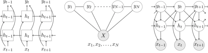
Figure 1: Graphical depictions of BiLSTMs (left), conditional random fields (middle) and refinement hidden Markov models (right). In practice, for the R-HMMs and CRFs we use a trigram model and not a bigram model as depicted.
decoded string that has the same context as the one found before, for instance, the stringslaywe would haveσ(4,slay) = 1.
For all contexts, we calculate (based on the training data) a frequency table, that gives the probability of an insertion given the specific context. In some cases, we then tune a threshold (based on a development set) so that we add insertions only in cases where the frequency is larger than that threshold. We found out that while it perhaps prevents insertions in legitimate positions, if the frequency threshold is low enough, it does not have an adverse effect. On the contrary, it prevents adding spurious insertions that cannot be correctly recovered as deletions. For more details, see§4.
In the morphology tasks we experiment with, insertions tend to happen as suffixes or prefixes. To capture this, we also learn a pair of thresholdsτ0andτ1 (by grid search on the training set) such that
σ(i, x)is set to0ifτ0≤
i
|x| ≤τ1.
Learning the Labeling Model withσ Once we have theσfunction applied to all aligned training data, we mark in theoutputsequences in the training data the spurious insertions that should not be in the input sequence with a special symbolD(for deletion). Therefore, the learning algorithm is now also required to learn where to delete these extra insertions thatσelicits. For example, if we consider the previously mentioned example ofsayandsaid, the input sequence in this case would besayεand the output sequence would besaid. However, it is not always the case that the past tense of a verb with aayending is the same word root with the suffix-d(and the transformation of the finalytoito accommodate the new suffix). For example, the past tense ofmayis alsomay, and in this case, if the stringmaywas also in the training set,mayshould retain its form and be transduced tomay. With the context function mentioned above we would have the pairmayε(input sequence),mayD(output sequence) to learn from. During decoding, we apply theσfunction on the input string and then remove theDsymbols from the string.
3.2 Sequence Labeling Models
We experiment with three models for sequence labeling: refinement hidden Markov models (R-HMMs; Stratos et al., 2013), conditional random fields (CRFs; Lafferty et al., 2001) and bidirectional Long Short Term Memory neural networks (biLSTMs; Graves and Schmidhuber, 2005). A graphical depiction of the models that we experiment with is given in Figure 1. For R-HMMs, we experiment with two learning algorithms, the expectation-maximization algorithm (EM; Dempster et al., 1977) and an L-PCFG spectral learning algorithm (Cohen et al., 2012; Cohen et al., 2013).3
4 Experiments
We describe in this section a set of experiments on datasets from three problems: social media spelling correction, optical character recognition (OCR) correction and morphological inflection. We believe that this array of datasets represents a broad set of problems in which string transduction as sequence
labeling can be tested. We apply the insertion technique to a set of sequence labelers: conditional random fields, refinement HMMs with expectation-maximization, spectral algorithms, and neural networks with biLSTM. All the results reported are at word level.
Our experiments require hyperparameter tuning of all algorithms, which we do over a fixed set of hyperparameters in the development set. For the latent-variable models, we vary the number of latent states between1and48. For the biLSTM, we try a number of layers between1and4and a number of neurons ranging between100and500.
The CRF is used with trigram modeling, and as such, the features it uses are very similar to the features used by the spectral algorithm. The main difference is that the spectral algorithm uses these features only during training, while the CRF uses them both during training and decoding.
In addition, we compare all our models to a seq2seq model implementation (Bahdanau et al., 2015). The model includes an attention mechanism, and we optimize the number of latent units over the development sets, ranging it from10to100. We also include a comparison to seq2seq models with a “hard” attention mechanism (Aharoni and Goldberg, 2017), designed for string transduction with monotonic alignments.
4.1 Twitter Spelling Correction
In our first set of experiments, we use a corpus of spelling corrections for Twitter (Aramaki, 2010). The corpus includes 39,172 words in their original form and their correct form. We split this dataset into three parts (consecutively): 31,172 entries for a training set, 4,000 entries for a development set and another 4,000 entries for a test set.
Further Tuning In our experiments with EM and the spectral algorithm, we also tried to tune theσ
context function on the development set. We discovered that the best context function is the one that adds
εslots for every contexta−bthat appears in the data, if the relative frequency ofa−btoa ? bis larger thanp= 0.0001(where?stands for a wildcard; the interpretation of this relative frequency division is that we check whether the conditional probability of having anεgiven the contexta ? bis larger thanp). This is not particularly surprising given the fact that the Twitter dataset is composed of single words, each having a single typo. Therefore, each pair of misspelled and correctly spelled words often needs at most one insertion to be aligned. Even though this threshold may seem small, it was enough to remove all the isolated, non-representative context cases.
We try both a bigram and a trigram model. The trigram model greatly outperforms the bigram model, so we focus on it. We also did some preliminary experiments with a4-gram model, but this model did not seem to do better than the trigram model. For the biLSTM architecture, we find on the development set that the smallest error is with2layers and350neurons.
In our experiments, we compare two latent-variable learning methods: the EM algorithm and the spectral algorithm described by Stratos et al. (2013). EM was run for 8 iterations – in some preliminary experiments where we ran EM for much longer, we noticed it converges after very few iterations. We then choose the iteration that gave the best result on the development set. We range the number of latent states,
m, between2and48.
The Dictionary Layer We also experiment with an additional layer that we add to our transduction algorithm. In this layer, we use a dictionary (a fixed set of words) for which we find the closest entry (in edit distance) to the output of our algorithm. In that case, our transduction algorithm can be thought of as producing anintermediatestring, i.e., a string that may or may not already be a correct word but that is closer to the correct word in terms of edit distance. The intermediate string representation is intended to correct mistakes while actually relying on the type of substitutions, deletions and insertions done by users of social media. However, it is still prone to character-based mistakes, since it is a learned component. This is the reason why we also include the second edit distance layer.
We use two types of dictionaries. The first dictionary is the set of all correctly spelled words in the training data. The second dictionary is the English dictionary extracted from the GNU aspell software.4 In our results, we report four types of accuracy levels: the accuracy for the whole test set (where accuracy
method acc acc4+ acc6+ acc10+
aspell 30.1 41.1 56.6 82.6
train 40.1 59.6 71.6 71.9
GNU aspell 29.0 46.2 58.8 80.2
seq2seq 46.3 44.8 45.3 33.8
seq2seq+train 55.7 59.5 65.1 86.2
seq2seq+aspell 47.6 48.5 45.0 65.4 seq2seq (hard) 52.2 49.1 31.6 13.4 seq2seq+train (hard) 62.2 63.6 59.6 63.8 seq2seq+aspell (hard) 54.9 53.3 47.1 63.8
Spectral 54.3 52.6 44.0 28.1
Spectral+train 63.3 68.4 70.1 69.4 Spectral+aspell 56.6 59.4 58.6 70.2
biLSTM 54.1 54.1 55.4 49.3
biLSTM+train 64.6 64.6 68.7 72.1
biLSTM+aspell 56.9 57.0 59.1 63.0
CRF 34.2 34.2 32.2 19.0
CRF+train 55.9 55.9 59.5 67.8
CRF+aspell 45.2 45.2 46.4 50.8
EM 28.3 22.0 14.5 9.9
EM+train 52.8 64.0 70.8 72.7
[image:6.595.170.429.59.362.2]EM+aspell 41.7 48.7 55.7 82.6
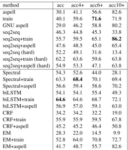
Table 1: Final results on the test set for the Twitter dataset. “aspell” stands for edit distance minimization using the aspell dictionary. “train” stands for the same with the dictionary extracted from the training set. “GNU aspell” stands for the results of running the GNU aspell software. “acc” denotes the accuracy over the whole dev/test set, “accn+” for words of length≥n. For each method the best model was chosen as follows: for CRF, over the dictionary; for EM, over iterations, number of latent states, and dictionary; and for spectral, over the hyperparameters, number of latent states and dictionary. The best model was chosen for each accuracy length criterion separately. The best result in each column is in bold. Top part are baselines. Bottom part uses our reduction to sequence labeling.
is measured as the number of words we fixed to the correct form), and also accuracy only for (correct) words which are longer than 4 characters, 6 characters and 10 characters.
We experimented with two types of edit distance algorithms. The first one allows only deletions, insertions and substitutions, and the other also allows transpositions. We discovered that edit distance with transposition behaves better, so we focus on it.
Results Table 1 gives the final result on the test set for the Twitter data (for different word lengths). The first thing to note is that there are some models that perform well on words longer than 10 characters. In general, it is easier to correct the spelling of longer words with the aspell dictionary because: (a) longer words are more likely to originate in words that appear in the dictionary; (b) there is more evidence in a long string for the misspelled string than in a short string.
Still, high accuracy on long words does not necessarily indicate the total accuracy is higher. We see that the spectral algorithm and the biLSTM model tend to give higher results on all words lengths overall than both the conditional random field and the EM algorithm. The GNU aspell software itself does not perform well on this dataset. This perhaps should not come as a surprise, as the GNU aspell software is designed for less informal text.
context dictionary average std
left none 42.2 0.67
right none 42.1 0.63
both none 42.3 0.61
left aspell 48.6 0.52
right aspell 48.6 0.54
both aspell 48.8 0.56
left train 58.3 0.49
right train 58.3 0.27
[image:7.595.211.390.61.199.2]both train 58.6 0.46
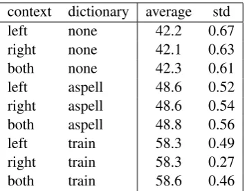
Table 2: Sensitivity analysis of the different context functions as a function of the probability threshold for insertion in a context. The contexts vary over left character (“left”), right character, or characters both on the left and the right (“both”). In addition, we use dictionaries (the aspell dictionary or the training data as dictionary). “average” gives the average result over the different thresholds, and “std” gives the standard deviation of that average.
especially for long words.
The Role of the Context Function We note that the choice of the context function is important, and extraεsymbols have to be added based on data-oriented choices. For example, when we experimented with a constant context function that adds an additionalεsymbol after every character during training and decoding, the accuracy on the test set was much lower, whether we used a dictionary or not. To be more precise, the accuracy without using a dictionary was 33%, with the “train” dictionary mitigating the low performance to an accuracy of 61.1% (which is significantly lower than the biLSTM result and the spectral result) and 54.0% for the “aspell” dictionary.
To test the role of the context function, we further evaluated it more thoroughly. We created three types of context functions: one that looks at context only to the left of the current character, one that looks at context only on the right, and finally one that looks on context both on the left and on the right (as originally defined). In addition, we varied the threshold that activates an insertion in a specific context (see §3). The threshold was varied over the values in the set{0.0001,0.0005,0.001,0.002,0.005,0.01,0.05,
0.1,0.15,0.2}. The higher the threshold is, the less spurious insertions happen (or insertions in general). We experimented with a single learning algorithm: the biLSTM neural network. Table 2 summarizes this sensitivity analysis. The “average” results give the performance on the development set, averaging over the different thresholds. The “std” result gives the corresponding standard deviation. As can be seen, on average, right context functions have smaller standard deviation than other contexts, while the accuracy levels are similar for all contexts. In addition, there is relatively not a very large sensitivity to the actual threshold use.
The same dataset was also used by Cotterell et al. (2014) and by Silfverberg et al. (2016) though in both cases the results are not comparable as the experimental setup and the errors reported are different than the one used in this paper. For example, Cotterell et al. do not report accuracy at all, but instead plot mean edit distance as a function of the number of training examples.
4.2 Optical Character Recognition Correction
Method acc acc4+ acc6+ acc10+
Unstructured 20.0 - -
-+ Lexicon 21.6 - -
-Perceptron 32.1 - -
-+ Lexicon 35.1 - -
-seq2seq 79.9 80.0 78.8 78.6
seq2seq (hard) 58.4 55.4 55.3 53.7
Spectral 77.3 77.9 76.3 73.8
CRF 81.8 81.9 80.7 78.8
EM 79.9 80.5 79.3 77.4
[image:8.595.187.412.61.214.2]biLSTM 81.7 81.7 80.3 78.3
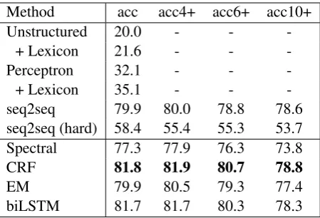
Table 3: Finnish OCR results. The first set of baselines (upper part) are reported by Silfverberg et al. (2016), and as such, the numbers are not available for all columns. Bottom part is our method.
Further Tuning In our experiments, we use 10-fold cross validation. The results are averaged over these ten folds. The hyperparameters for the spectral algorithm were tuned on the development set of the first fold, and then we used the hyperparameters identified at that phase for the rest of the folds.
We tuned the neural network architecture parameters on the development set of the first fold. We found out that the biLSTM model works best with1layer with200neurons.
We tuned the context function on development data again (for fold1). We discovered that the best context function includes a pair ofεin any context of the forma− −bthat it appeared in the training data, and a singleεin any context with conditional probability larger than0.0001. See more in§4.1. The OCR dataset is quite different in its structure from the Twitter dataset. It has both words that do not need any correction, and words in which more than one character was not labeled with the correct character. Another important difference is the fact the “typos” were often grammatical in the Twitter dataset (as they were human misspellings), while that is not the case in the OCR dataset. It is also worth noting that Finnish relies heavily on double letters in its spelling, which could explain why this choice ofσfunction works best in this case but not in the Twitter one.
Silfverberg et al. (2016) present two approaches for this problem, both relying on finite-state technology. In one approach, “unstructured,” they extract finite-state rules from pairs of strings and then apply them during decoding. In the “structured” case there is an additional Perceptron layer which is trained based on features extracted from the unstructured classifier. In addition, they have an additional layer which relies on a lexicon to find the best correction for a given input string.
Results Table 3 gives the results. We see that all uses of sequence labeling significantly outperform the results of Silfverberg et al. (2016). Even with an external lexicon, the results of the unstructured and structured classifiers of Silfverberg et al. significantly lag behind our results. Our results are also relatively stable with regards to word length. While the results are slightly lower for words of length 10 or more, the accuracy level is rather stable for other lengths. This is actually a different finding than the one we found with the Twitter spelling correction experiment. We see yet again that seq2seq modeling performs worse than our approach with biLSTM. seq2seq do not perform well with the hard monotonic attention model. This is on par with the results for the Twitter spelling dataset, on which we see bad behavior on long words. The OCR dataset indeed includes relatively long words.
4.3 Morphological Inflection
We also run experiments on the morphological inflection dataset used by Rastogi et al. (2016).5 This dataset was first processed by Dreyer (2011) and we use the same setup in our experiments, i.e., in each experiment we use the same 2,500 example dataset sampled from the CELEX database (Baayen et al., 1993) divided into three sets, 500 examples for training, and 1,000 for both development and testing. This
Model 13SIA 2PIE 2PKE rP
biLSTM-WFST 85.1 94.4 85.5 83.0
biLSTM (ensemble) 85.8 94.6 86.0 83.8
Moses15 85.3 94.0 82.8 70.8
Dreyer (Backoff) 82.8 88.7 74.7 69.9 Dreyer (Lat-Class) 84.8 93.6 75.7 81.8 Dreyer (Lat-Region) 87.5 93.4 87.4 84.9
Kann (MED) 82.3 94.4 86.8 83.9
Kann (MED+POET) 83.9 95.0 87.6 84.0
seq2seq 83.1 93.8 88 83.2
seq2seq (hard) 85.8 95.1 89.5 87.2
EM 68.5 93.5 77.2 75.8
biLSTM (ours) 80.2 93.8 84.2 83.0
CRF 79.2 88.1 72.4 84.7
Spectral 81.9 94.0 83.2 83.8
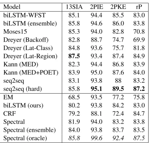
[image:9.595.176.423.58.295.2]Spectral (ensemble) 84.0 93.8 83.7 83.5 Spectral (oracle) 85.8 99.6 92.4 87.5
Table 4: Results on the morphological inflection datasets. Baselines (upper part of the table) are reported by Rastogi et al. (2016) and Dreyer (2011). The best result in each column is in bold. Results for seq2seq are reported by Aharoni and Goldberg (2017). Kann results are reported by Kann and Sch¨utze (2016).
corpus is divided in four subsets, each defining an inflection task between different verb tenses in German. These are labeled as follows:
• 13SIA→13SKE - 1st/3rd persons singular of the indicative past to 1st/3rd persons singular of the subjunctive present.
• 2PIE→13PKE - 2nd person plural of the indicative present to 1st/3rd person plural of the subjunctive present.
• 2PKE→z - 2nd person plural of the subjunctive present to the infinitive. • rP→pA - imperative plural to the past participle.
Further Tuning For the 13SIA dataset, we discovered on development data (fold1) that the best context function is one that adds a singleεany time it appeared in the training data with a contextaεb. For 2PIE, we discovered similarly that adding a singleεis best in all cases it appears in the end of the word in the training set. Finally, for 2PKE and rP, we discovered the best context function is such that it adds a single
εor a pair ofεin any context it appears in the training data (with a character to the left and a character to the right).
The morphological inflection dataset is the most different of the three datasets mostly because it allows for the insertion or deletion of full suffixes. We speculate it is the main factor as to why the best context functions for the morphological datasets are different than for the previous two datasets (Twitter and OCR).
With the biLSTM model we discovered on the development set of the first fold of each dataset that: 13SIA works best with2layers of size300; 2PIE works best with1layer of size150; 2PKE works best with1layer of size250; and rP-pA works best with2layers of size250.
Results The results are in Table 4. The biLSTM results reported in the upper part of the table do not use our sequence labeling technique, and are re-iterated as reported by Rastogi et al. (2016).
An additional observation is that the way we handle insertions has a significant impact on the perfor-mance. In oracle mode (meaning, when the two strings are aligned using edit distance even at decoding time, and the spurious insertions are not used), the spectral algorithm performs significantly better. This should not come as a surprise, but does point to a direction on how to improve the use of our sequence labeling technique – better handling of insertions and the addition of less spurious insertion placeholders that are deleted during decoding.
In contrast to the other datasets, where perhaps the assumption of monotonicity is too strong, seq2seq models with an attention mechanism designed to handle monotonic alignments (Aharoni and Goldberg, 2017) perform quite well on this task, even better than the vanilla seq2seq models.
Finally, we also consider the case in which we use an ensemble method, combining several spectral models together (the top 50 performing models on the development set from the hyperparameter sweep). We combine the models using a MaxEnt reranker such as described by Charniak and Johnson (2005) and Narayan and Cohen (2015). We find that the ensemble approach does improve the results significantly for the 13SIA dataset, and also for the 2PKE-z dataset.
5 Conclusion
We presented a technique to frame general string transduction problems as sequence labeling. Our technique works by adding to the string to be transduced additional insertion markers, which are later potentially deleted during the sequence labeling process. Our approach is general and works with any sequence labeling algorithm. We developed our technique with conditional random fields, refinement hidden Markov models and neural networks. We tested our approach on problems from three challenging domains: spelling correction for social media, optical character recognition correction and morphological inflection. We demonstrated that our approach performs comparably to strong baselines and state of the art.
While the idea of using redundant epsilons in string transduction problems has been used in the past (Azawi et al., 2013; Schnober et al., 2016), it has traditionally been treated in an ad-hoc narrow manner, for example by adding a fixed number of epsilons after every character. To the best of our knowledge, we are the first to rigorously define this idea as a learning problem while performing a comprehensive empirical evaluation for it, both with respect to the type of datasets used and the sequence labeling algorithms covered.
Acknowledgements
We would like to thank Ariadna Quattoni, Adam Lopez and other members of the Edinburgh NLP group for their feedback and comments on this paper. We would also like to thank Tao Meng for his help with running the BiLSTM experiments. We gratefully acknowledge the support of the the European Union under the Horizon 2020 SUMMA project (grant agreement 688139), and the support of EPSRC (award number 1644752).
References
Roee Aharoni and Yoav Goldberg. 2017. Morphological inflection generation with hard monotonic attention. In
Proceedings of the 55th Annual Meeting of the Association for Computational Linguistics, pages 2004–2015, Vancouver, Canada.
Cyril Allauzen, Michael Riley, Johan Schalkwyk, Wojciech Skut, and Mehryar Mohri. 2007. OpenFst: A general and efficient weighted finite-state transducer library. InProceedings of the 12th International Conference on Implementation and Application of Automata, Lecture Notes in Computer Science, pages 11–23, Prague, Czech Republic.
Eiji Aramaki. 2010. Typo corpus. Available athttp://luululu.com/tweet/#cr.
Harald R. Baayen, Richard Piepenbrock, and Hedderik van Rijn. 1993. The CELEX lexical data base on CD-ROMs. Linguistic Data Consortium, University of Pennsylvania.
Dzmitry Bahdanau, Kyunghyun Cho, and Yoshua Bengio. 2015. Neural machine translation by jointly learning to align and translate. InProceedings of the 3rd International Conference on Learning Representations, San Diego, California, USA.
Raphael Bailly, Xavier Carreras, and Ariadna Quattoni. 2013. Unsupervised spectral learning of finite state transducers. InAdvances in Neural Information Processing Systems 26, pages 800–808.
Jane Chandlee. 2014.Strictly local phonological processes. Ph.D. thesis, Department of Linguistics and Cognitive Science, University of Delaware.
Eugene Charniak and Mark Johnson. 2005. Coarse-to-finen-best parsing and maxent discriminative reranking. InProceedings of the 43rd Annual Meeting on Association for Computational Linguistics, pages 173–180, Ann Arbor, Michigan.
Alexander Clark. 2001. Partially supervised learning of morphology with stochastic transducers. InProceedings of the 6th Natural Language Processing Pacific Rim Symposium, pages 341–348, Tokyo, Japan.
Shay B. Cohen, Karl Stratos, Michael Collins, Dean P. Foster, and Lyle Ungar. 2012. Spectral learning of latent-variable PCFGs. InProceedings of the 50th Annual Meeting of the Association for Computational Linguistics, pages 223–231, Jeju Island, Korea.
Shay B. Cohen, Karl Stratos, Michael Collins, Dean P. Foster, and Lyle Ungar. 2013. Experiments with spectral learning of latent-variable PCFGs. InProceedings of the 2013 Conference of the North American Chapter of the Association for Computational Linguistics: Human Language Technologies, pages 148–157, Atlanta, Georgia.
Ryan Cotterell, Nanyun Peng, and Jason Eisner. 2014. Stochastic contextual edit distance and probabilistic FSTs. InProceedings of the 52nd Annual Meeting of the Association for Computational Linguistics, pages 625–630, Baltimore, Maryland.
Arthur Dempster, Natalie Laird, and Donald B. Rubin. 1977. Maximum likelihood estimation from incomplete data via the EM algorithm.Journal of the Royal Statistical Society B, 39:1–38.
Markus Dreyer, Jason Smith, and Jason Eisner. 2008. Latent-variable modeling of string transductions with finite-state methods. InProceedings of the 2008 Conference on Empirical Methods in Natural Language Processing, pages 1080–1089, Honolulu, Hawaii.
Markus Dreyer. 2011. A non-parametric model for the discovery of inflectional paradigms from plain text using graphical models over strings. Ph.D. thesis, Johns Hopkins University, Baltimore, MD.
Jason Eisner. 2002. Parameter estimation for probabilistic finite-state transducers. InProceedings of 40th Annual Meeting of the Association for Computational Linguistics, pages 1–8, Philadelphia, Pennsylvania, USA.
Alex Graves and J¨urgen Schmidhuber. 2005. Framewise phoneme classification with bidirectional LSTM and other neural network architectures. Neural Networks, 18(5):602–610.
Katharina Kann and Hinrich Sch¨utze. 2016. Single-model encoder-decoder with explicit morphological repre-sentation for reinflection. InProceedings of the 54th Annual Meeting of the Association for Computational Linguistics, pages 555–560, Berlin, Germany.
Kevin Knight and Jonathan Graehl. 1998. Machine transliteration. Computational Linguistics, 24(4):599–612.
Kimmo Koskenniemi. 1983. Two-level morphology. Ph.D. thesis, University of Helsinki.
Shankar Kumar, Yonggang Deng, and William Byrne. 2006. A weighted finite state transducer translation template model for statistical machine translation.Natural Language Engineering, 12(1):35–75.
John D. Lafferty, Andrew McCallum, and Fernando C. N. Pereira. 2001. Conditional Random Fields: Probabilistic models for segmenting and labeling sequence data. In Proceedings of the 18th International Conference on Machine Learning, pages 282–289, San Francisco, CA, USA.
Jordi Porta and Jos´e-Luis Sancho. 2013. Word normalization in Twitter using finite-state transducers. In Proceed-ings of the Tweet Normalization Workshop co-located with 29th Conference of the Spanish Society for Natural Language Processing, pages 49–53, Madrid, Spain.
Pushpendre Rastogi, Ryan Cotterell, and Jason Eisner. 2016. Weighting finite-state transductions with neural context. InProceedings of the 2016 Conference of the North American Chapter of the Association for Compu-tational Linguistics: Human Language Technologies, pages 623–633, San Diego, California.
Mihaela Rosca and Thomas Breuel. 2016. Sequence-to-sequence neural network models for transliteration.arXiv preprint:1610.09565.
Carsten Schnober, Steffen Eger, Erik-Lˆan Do Dinh, and Iryna Gurevych. 2016. Still not there? Comparing traditional sequence-to-sequence models to encoder-decoder neural networks on monotone string translation tasks. InProceedings of the 26th International Conference on Computational Linguistics, pages 1703–1714, Osaka, Japan.
Miikka Silfverberg, Pekka Kauppinenb, and Krister Lind´enb. 2016. Data-driven spelling correction using weighted finite-state methods. InProceedings of the ACL Workshop on Statistical NLP and Weighted Automata, pages 51–59, Berlin, Germany.