2493
Why does
PairDiff
work? – A Mathematical Analysis of
Bilinear Relational Compositional Operators for Analogy Detection
Huda Hakami
The University of Liverpool Liverpool, UK
Kohei Hayashi
Preferred Networks Tokyo, Japan
Danushka Bollegala
The University of Liverpool Liverpool, UK
Abstract
Representing the semantic relations that exist between two given words (or entities) is an im-portant first step in a wide-range of NLP applications such as analogical reasoning, knowledge base completion and relational information retrieval. A simple, yet surprisingly accurate method for representing a relation between two words is to compute the vector offset (PairDiff) between their corresponding word embeddings. Despite the empirical success, it remains unclear as to whetherPairDiffis the best operator for obtaining a relational representation from word embed-dings. We conduct a theoretical analysis of generalised bilinear operators that can be used to measure the`2 relational distance between two word-pairs. We show that, if the word
embed-dings are standardised and uncorrelated, such an operator will be independent of bilinear terms, and can be simplified to a linear form, where PairDiffis a special case. For numerous word embedding types, we empirically verify the uncorrelation assumption, demonstrating the general applicability of our theoretical result. Moreover, we experimentally discoverPairDifffrom the bilinear relational compositional operator on several benchmark analogy datasets.
1 Introduction
Different types of semantic relations exist between words such asHYPERNYMYbetweenostrichand
bird, orANTONYMYbetweenhotandcold. If we consider entities1, we can observe even a richer diver-sity of relations such asFOUNDER-OFbetweenBill GatesandMicrosoft, orCAPITAL-OF between
TokyoandJapan. Identifying the relations between words and entities is important for various Natural Language Processing (NLP) tasks such as automatic knowledge base completion (Socher et al., 2013), analogical reasoning (Turney and Littman, 2005; Bollegala et al., 2009) and relational information re-trieval (Duc et al., 2010). For example, to solve a word analogy problem of the form “ais tobascis to
?”, the relationship between the two words in the pair(a, b)must be correctly identified in order to find candidatesdthat have similar relations withc. For example, given the query “Bill Gatesis toMicrosoft
asSteve Jobsis to?”, a relational search engine must retrieveApple Inc. because theFOUNDER-OF relation exists between the first and the second entity pairs.
Two main approaches for creating relation embeddings can be identified in the literature. In the first approach, from given corpora or knowledge bases, word and relation embeddings arejointlylearnt such that some objective is optimised (Guo et al., 2016; Yang et al., 2015; Nickel et al., 2016; Bordes et al., 2013; Rocktäschel et al., 2016; Minervini et al., 2017; Trouillon et al., 2016). In this approach, word and relation embeddings are considered to beindependentparameters that must be learnt by the embedding method. For example, TransE (Bordes et al., 2013) learns the word and relation embeddings such that we can accurately predict relations (links) in a given knowledge base using the learnt word and relation embeddings. Because relations are learnt independently from the words, we refer to methods that are based on this approach asindependentrelational embedding methods.
This work is licensed under a Creative Commons Attribution 4.0 International Licence. Licence details: http://creativecommons.org/licenses/by/4.0/.
1We interchangeably use the terms
A second approach for creating relational embeddings is to apply some operator on two word embed-dings tocomposethe embedding for the relation that exits between those two words, if any. In contrast to the first approach, we do not have to learn relational embeddings and hence this can be considered as an unsupervised setting, where the compositional operator is predefined. A popular operator for composing a relational embedding from two word embeddings isPairDiff, which is the vector difference (offset) of the word embeddings (Mikolov et al., 2013b; Levy and Goldberg, 2014; Vylomova et al., 2016; Bolle-gala et al., 2015b; Blacoe and Lapata, 2012). Specifically, given two wordsaandbrepresented by their word embeddings respectivelyaandb, the relation betweenaandbis given bya−bunder thePairDiff operator. Mikolov et al. (2013b) showed that# » PairDiffcan accurately solve analogy equations such as
king−man# »+woman# »=queen# », where we have used the top arrows to denote the embeddings of the corresponding words. Bollegala et al. (2015a) showed thatPairDiffcan be used as a proxy for learning better word embeddings and Vylomova et al. (2016) conducted an extensive empirical comparison of PairDiffusing a dataset containing 16 different relation types. BesidesPairDiff, concatenation (Hakami and Bollegala, 2017; Yin and Schütze, 2016), circular correlation and convolution (Nickel et al., 2016) have been used in prior work for representing the relations between words. Because the relation em-bedding is composed using word emem-beddings instead of learning as a separate parameter, we refer to methods that are based on this approach ascompositionalrelational embedding methods. Note that in this approach it is implicitly assumed that there exist only a single relation between two words.
In this paper, we focus on the operators that are used in compositional relational embedding methods. If we assume that the words and relations are represented by vectors embedded in some common space, then the operator we are seeking must be able to produce a vector representing the relation between two words, given their word embeddings as the only input. Although there have been different proposals for computing relational embeddings from word embeddings, it remains unclear as to what is the best operator for this task. The space of operators that can be used to compose relational embeddings is open and vast. A space of particular interest from a computational point-of-view is the bilinear operators that can be parametrised using tensors and matrices. Specifically, we consider operators that consider pair-wise interactions between two word embeddings (second-order terms) and contributions from individual word embeddings towards their relational embedding (first-order terms). The optimality of a relational compositional operator can be evaluated, for example, using the expected relational distance/similarity such as`2between analogous (positive) vs. nonanalogous (negative) word-pairs.
If we assume that word embeddings are standardised, uncorrelated and word-pairs are i.i.d, then we prove in §3 that bilinear relational compositional operators are independent of bilinear pairwise interac-tions between the two input word embeddings. Moreover, under regularised settings (§3.1), the bilin-ear operator further simplifies to a linbilin-ear combination of the input embeddings, and the expected loss over positive and negative instances becomes zero. In §4.1, we empirically validate the uncorrelation assumption for different pre-trained word embeddings such as the Continuous Bag-of-Words Model (CBOW) (Mikolov et al., 2013a), Skip-Gram with negative sampling (SG) (Mikolov et al., 2013a), Global Vectors (GloVe) (Pennington et al., 2014), word embeddings created using Latent Semantic Anal-ysis (LSA) (Deerwester et al., 1990), Sparse Coding (HSC) (Faruqui et al., 2015; Yogatama et al., 2015), and Latent Dirichlet Allocation (LDA) (Blei et al., 2003). This empirical evidence implies that our theoretical analysis is applicable to relational representations composed from a wide-range of word em-bedding learning methods. Moreover, our experimental results show that a bilinear operator reaches its optimal performance in two different word-analogy benchmark datasets, when it satisfies the require-ments of thePairDiffoperator. We hope that our theoretical analysis will expand the understanding of relational embedding methods, and inspire future research on accurate relational embedding methods using word embeddings as the input.
2 Related Work
As already mentioned in §1, methods for representing a relation between two words can be broadly categorised into two groups depending on whether the relational embeddings are learnt independently
embeddings fully depend on the input word embeddings. Next, we briefly overview the different methods that fall under each category. For a detailed survey of relation embedding methods see Nickel et al. (2015).
Given a knowledge base where an entity h is linked to an entity t by a relation r, the TransE model (Bordes et al., 2013) scores the tuple(h, t, r) by the `1 or`2 norm of the vector(h+r−t).
Nickel et al. (2011) proposed RESCAL, which usesh>Mrtas the scoring function, whereMris a ma-trix embedding of the relationr. Similar to RESCAL, Neural Tensor Network (Socher et al., 2013) also models a relation by a matrix. However, compared to vector embeddings of relations, matrix embeddings increase the number of parameters to be estimated, resulting in an increase in computational time/space and likely to overfit. To overcome these limitations, DistMult (Yang et al., 2015) models relations by vectors and use elementwise multilinear dot productrht. Unfortunately, DistMult cannot capture directionality of a relation. Complex Embeddings (Trouillon et al., 2016) overcome this limitation of DistMult by using complex embeddings and defining the score to be the real part ofrh¯t, where¯t
denotes the complex conjugate oft.
The observation made by Mikolov et al. (2013b) that the relation between two words can be rep-resented by the difference between their word embeddings sparked a renewed interest in methods that compose relational embeddings using word embeddings. Word analogy datasets such as Google dataset (Mikolov et al., 2013b), SemEval 2012 Task2 dataset (Jurgens et al., 2012), BATS (Drozd et al., 2016) etc. have established as benchmarks for evaluating word embedding learning methods.
Different methods have been proposed to measure the similarity between the relations that exist be-tween two given word pairs such asCosMult,CosAddandPairDiff(Levy and Goldberg, 2014; Bolle-gala et al., 2015a). Vylomova et al. (2016) studied as to what extent the vectors generated using simple PairDiff encode different relation types. Under supervised classification settings, they conclude that PairDiffcan cover a wide range of semantic relation types. Holographic embeddings proposed by Nickel et al. (2016) use circular convolution to mix the embeddings of two words to create an embedding for the relation that exist between those words. It can be showed that circular correlation is indeed an elemen-twise product in the Fourier space and is mathematically equivalent to complex embeddings (Hayashi and Shinbo, 2017).
Although PairDiffoperator has been widely used in prior work for computing relation embeddings from word embeddings, to the best of our knowledge, no theoretical analysis has been conducted so far explaining why and under what conditionsPairDiffis optimal, which is the focus of this paper.
3 Bilinear Relation Representations
Let us consider the problem of representing the semantic relation r(h,t) between two given wordsh
andt. We assume that h andt are already represented in some d-dimensional space respectively by their word embeddings h,t ∈ Rd. The relation between two words can be represented using differ-ent linear algebraic structures. Two popular alternatives are vectors (Nickel et al., 2016; Bordes et al., 2013; Minervini et al., 2017; Trouillon et al., 2016) and matrices (Socher et al., 2013; Bollegala et al., 2015b). Vector representations are preferred over matrix representations because of the smaller number of parameters to be learnt (Nickel et al., 2015).
Let us assume that the relation r is represented by a vector r ∈ Rδ in some δ-dimensional space.
Therefore, we can writer(h,t)as a function that takes two vectors (corresponding to the embeddings of the two words) as the input and returns a single vector (representing the relation between the two words) as given in (1).
r:Rd×Rd→Rδ (1)
Having both words and relations represented in the sameδ=ddimensional space is useful for perform-ing linear algebraic operations usperform-ing those representations in that space. For example, in TransE (Bordes et al., 2013), the strength of a relationr that exists between two wordsh andtis computed as the`1,2
same vector space. Ifδ < d, we can first project word embeddings to a lowerδ-dimensional space using some dimensionality reduction method such as SVD, whereas ifδ >dwe can learn higherδ-dimensional overcomplete word representations (Faruqui et al., 2015) from the originald-dimensional word embed-dings. Therefore, we will limit our theoretical analysis to theδ=dcase for ease of description.
Different functions can be used asr(h,t)that satisfy the domain and range requirements specified by (1). If we limit ourselves to bilinear functions, the most general functional form is given by (2).
r(h,t) =h>At+Ph+Qt (2)
Here, A ∈ Rd×d×d is a 3-way tensor in which each slice is a d×dreal matrix. Let us denote the k-th slice ofAbyA(k) and its(i, j) element byA(ijk). The first term in (2) corresponds to the pairwise interactions betweenhandt.P,Q∈Rd×dare the nonsingular2projection matrices involving first-order contributions respectively ofhandttowardsr.
Let us consider the problem of learning the simplest bilinear functional form according to (2) from a given dataset of analogous word-pairsD+ ={((h, t),(h0, t0))}. Specifically, we would like to learn the
parametersA,PandQsuch that some distance (loss) between analogous word-pairs is minimised. As a concrete example of a distance function, let us consider the popularly used Euclidean distance3(`2loss)
for two word pairs given by (3).
J((h, t),(h0, t0)) =
r(h,t)−r(h0,t0)
2
2 (3)
If we were provided only analogous word-pairs (i.e. positive examples), then this task could be trivially achieved by setting all parameters to zero. However, such a trivial solution would not generalise to unseen test data. Therefore, in addition toD+ we would require a set of non-analogous word-pairsD−
as negative examples. Such negative examples are often generated in prior work by randomly corrupting positive relational tuples (Nickel et al., 2016; Bordes et al., 2013; Trouillon et al., 2016) or by training an adversarial generator (Minervini et al., 2017).
The total lossJover both positive and negative training data can be written as follows:
J= X
((h,t),(h0,t0))∈D+
r(h,t)−r(h
0
,t0) 2 2− X
((h,t),(h0,t0))∈D−
r(h,t)−r(h
0
,t0)
2
2 (4)
Assuming that the training word-pairs are randomly sampled from D+ and D− according to two
distributions respectivelyp+andp−, we can compute the total expected loss,Ep[J], as follows:
Ep[J] =Ep+
h
r(h,t)−r(h0,t0) 2 2 i
−Ep−
h
r(h,t)−r(h0,t0) 2 2 i (5)
We make the following assumptions to further analyse the properties of relational embeddings.
Uncorrelation: The correlation between any two distinct dimensions of a word embedding is zero. One
might think that the uncorrelation of word embedding dimensions to be a strong assumption, but we later show its validity empirically in §4.1 for a wide range of word embeddings.
Standardisation: Word embeddings are standardised to zero mean and unit variance. This is a linear
transformation in the word embedding space and does not affect the topology of the embedding space. In particular, translating word embeddings such that they have a zero mean has shown to improve performance in similarity tasks Mu et al. (2018).
Relational Independence Word pairs in the training data are assumed to be i.i.d. For example, whether
a particular semantic relationrexists between handt, is assumed to be independent of any other relationr0 that exists betweenh0 andt0 in a different pair. For example, (ostrich,is-a-large,bird) is independent from (Trump,president-of,USA).
2
If the projection matrix is nonsingular, then the inverse projection exists, which preserves the dimensionality of the embed-ding space.
3For`
For relation representations given by (2), 1 holds:
Theorem 1. Consider the bilinear relational embedding defined by 2 computed using uncorrelated word
embeddings. If the word embeddings are standardised, then the expected loss given by 5 over a relation-ally independent set of word pairs is independent ofA.
Proof. Let us consider the bilinear term in (2), becauseiandj(6=i)dimensions of word embeddings are uncorrelated by the assumption (i.e. corr(ui, uj) = 0), from the definition of correlation we have,
corr(ui, uj) =E[uiuj]−E[ui]E[uj] = 0 (6)
E[uiuj] =E[ui]E[uj]. (7)
Moreover, from the standardisation assumption we have,E[ui] = 0, ∀i=1...n. From (7) it follows that:
E[uiuj] = 0 (8)
fori6=jdimensions.
We will next show that (5) is independent ofA. For this purpose, let us consider theEp+ term first and
write thek-th dimension ofr(h,t)usingA(k),PandQas follows:
X
i,j
A(ijk)hitj
+X
n
Pknhn+
X
n
Qkntn (9)
Plugging (9) in (5) and computing the loss over all positive training instances we get,
Ep+[
X
k
(X
i,j
A(ijk)(hitj−h0it
0
j)
+X
n
Pkn(hn−h0n) +
X
n
Qkn(tn−t0n))
2
] (10)
Terms that involve only elements inA(k)take the form:
X
i,j
X
l,m
Ep+
h A(ijk)A
(k)
lm(hitj−h
0
it
0
j)(hltm−h0lt
0 m) i =X i,j X l,m
A(ijk)A(lmk)(Ep+[hitjhltm]−Ep+[hitjh
0
lt
0
m]−Ep+[h
0
it
0
jhltm] +Ep+[h
0 it 0 jh 0 lt 0
m]) (11)
Lets first analyse the cases wherei6=jandl6= m. Because of the relational independence assump-tion, the second and the third expectations in (11) can be written as follows: Ep+[hitj]Ep+[h
0 lt
0 m]and
Ep+[h
0
it0j]Ep+[hltm], respectively. Each of the these expectations contains the product of different
di-mensionalities in two different words. Expected correlation of different dimensions in the same word is zero from (8). Therefore, such cross-correlations are likely to be small for different word pairs, which are nonsynomyous. On the other hand, first and fourth expectations in (11) involve the same pair of words. For example, we could write the first expectation as follows:
Ep+[hitjhltm] =Ep+[(hihl)(tjtm) =Ep+[HilTjm]
where H = hihl and Tjm = tjtm. If we think ofH and T asd2-dimensional word embeddings,
Ep+[HilTjm]represents the expectation over two distinct dimensions ofH andT foril6=jm.
There-fore, from the same logic as above, this expectation is approximately zero.4 Fori=j =l=mcase we have,
A(ijk)2(Ep+[h
2
it
2
i]−2Ep+[hitih
0
it
0
i] +Ep+[h
0
i
2
t0i
2
]) (12)
4Note thatilcould be equal tojmeven wheni6=jandl6=m. However, such cases will be a rare minority. Nevertheless,
Because we are considering word-pairs (h,t) for which a relationris known to hold, from the definition of the correlation between the same dimension in different words we have:
corr(h2i, t2i) =E[h2it2i]−E[h2i]E[t2i] = 1
E[h2it2i] =E[h2i]E[t2i] + 1
BecauseE[h2i] =E[t2i] = 1from the standardisation, we get:
E[h2it2i] = 2 (13)
Lets analyse the second term in (12). From the relational independence and because the word embeddings are assumed to be standardised to unit variance, we obtain the follows:
2Ep+[hitih
0
it0i] = 2Ep+[hiti]Ep+[h
0
it0i] = 2. (14)
According to (13) and (14), (12) evaluates to2A(ijk)2. We will then get the same term from the negative
expectations and they would cancel out as2A(ijk)2is independent of the training dataset. Next, lets consider theA(ijk)Pknterms in the expansion of (10) given by,
2X
i,j
X
n
A(ijk)Pkn(hitj−h0it0j)(hn−h0n). (15)
Taking the expectation of (15) w.r.t.p+we get,
2X
i,j
X
n
A(ijk)Pkn(Ep+[hitjhn]−Ep+[hitjh
0
n]−Ep+[h
0
it
0
jhn] +Ep+[h
0
it
0
jh
0
n]). (16)
Likewise, from the uncorrelation assumption and following the same logic as above it follows that all the expectations in (16) are approximately zero. A similar argument can be used to show that terms that involve A(ijk)Qkn disappear from (10). Therefore, A does not play any part in the expected loss
over positive examples. Similarly, we can show thatAis independent of the expected loss over negative examples. Therefore, from (5) we see that the expected loss over the entire training dataset is independent ofA.
3.1 Regularised`2 loss
As a special case, if we attempt to minimise the expected loss under some regularisation onAsuch as the Frobenius norm regularisation, then this can be achieved by sendingAto zero tensor because according to 1 2 is independent fromA.
WithA=0, the relation betweenhandtcan be simplified to:
r(h,t) =Ph+Qt (17)
Then the expected loss over the positive instances is given by (18).
Ep+[
P(h−h
0
) +Q(t−t0)
2 2]
=Ep+[(h−h 0
)>P>P(h−h0)] +Ep+[(h−h 0
)>P>Q(t−t0)]+ Ep+[(t−t
0
)>Q>P(h−h0)] +Ep+[(t−t 0
)>Q>Q(t−t0)] (18)
The second expectation term in the right hand side of (18) can be computed as follows:
Ep+[(h−h 0
)>P>Q(t−t0)] =X
i,j
(P>Q)ijEp+[(hi−h
0
i)(tj−t0j)]
=X
i,j
(P>Q)ij Ep+[hitj]−Ep+[hit
0
j]−Ep+[h
0
itj] +Ep+[h
Wheni6=j, each of the four expectations in the RHS of (21) are zero from the uncorrelation assumption. When i = j, each term will be equal to one from the standardisation assumption (unit variance) and cancel each other out. A similar argument can be used to show that the third expectation term in the RHS of (18) vanishes.
Now lets consider the first expectation term in the RHS of (18), which can be computed as follows:
Ep+[(h−h 0
)>P>P(h−h0)] =X
i,j
(P>P)ijEp+[(hi−h
0
i)(hj−h0j)]
=X
i,j
(P>P)ij(Ep+[hihj]−Ep+[hih
0
j]−Ep+[h
0
ihj] +Ep+[h
0
ih
0
j]) (20)
Wheni6=j, it follows from the uncorrelation assumption that each of the four expectation terms in the RHS of (20) will be zero. Fori=jcase we have,
X
i,j
(P>P)iiEp+[h
2
i]−2Ep+[hih
0
i] +Ep+[h
0
i
2
]
= 2X
i,j
(P>P)ii (21)
Note that from the relational independence between h andh0 we have Ep+[hih
0
i] = Ep+[hi]Ep+[h
0 i].
From the standardisation (zero mean) assumption this term is zero. On the other hand Ep+[h 2
i] =
Ep+[h
0 i
2
] = 1from the standardisation (unit variance) assumption, which gives the result in (21). Similarly, the fourth expectation term in the RHS of (18) evaluates to2P
i,j(Q>Q)ii, which shows
that (18) evaluates to2P
i,j (P>P)ii+ (Q>Q)ii
. Note that this is independent of the positive instances and will be equal to the expected loss over negative instances, which givesEp[J] = 0for the relational
embedding given by (17).
It is interesting to note thatPairDiffis a special case of (17), whereP=IandQ=−I. In the general case where word embeddings are nonstandardised to unit variance, we can setPto be the diagonal matrix wherePii= 1/σi, whereσiis the variance of thei-th dimension of the word embedding space, to enforce
standardisation. Considering thatP,Qare parameters of the relational embedding, this is analogous to
batch normalisation(Ioffe and Szegedy, 2015), where the appropriate parameters for the normalisation are learnt during training.
4 Experimental Results
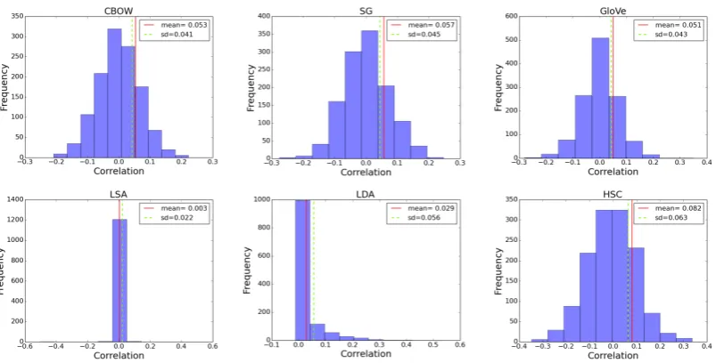
4.1 Cross-dimensional Correlations
A key assumption in our theoretical analysis is the uncorrelations between different dimensions in word embeddings. Here, we empirically verify the uncorrelation assumption for different input word embed-dings. For this purpose, we create SG, CBOW and GloVe embeddings from the ukWaC corpus5. We use a context window of 5 tokens and select words that occur at least 6 times in the corpus. We use the publicly available implementations for those methods by the original authors and set the parameters to the recommended values in (Levy et al., 2015) to create50-dimensional word embeddings. As a repre-sentative of counting-based word embeddings, we create a word co-occurrence matrix weighted by the positive pointwise mutual information (PPMI) and apply singular value decomposition (SVD) to obtain
50-dimensional embeddings, which we refer to as the Latent Semantic Analysis (LSA) embeddings. We use Latent Dirichlet Allocation (LDA) (Blei et al., 2003) to create a topic model, and represent each word by its distribution over the set of topics. Ideally, each topic will capture some semantic category and the topic distribution provides a semantic representation for a word. We use gensim6to extract50topics from a 2017 January dump of English Wikipedia. In contrast to the above-mentioned word embeddings,
5
http://wacky.sslmit.unibo.it/doku.php?id=corpora
Figure 1: Cross-dimensional correlations for six word embeddings
which are dense and flat structured, we used Hierarchical Sparse Coding7(HSC) (Yogatama et al., 2015) to produce sparse and hierarchical word embeddings.
Given a word embedding matrix W ∈ Rm×d, where each row correspond to the d-dimensional em-bedding of a word in a vocabulary containingm words, we compute a correlation matrixC ∈ Rd×d,
where the(i, j) element,Cij, denotes the Pearson correlation coefficient between the i-th andj-th
di-mensions in the word embeddings over them words. By constructionCii = 1and the histograms of
the cross-dimensional correlations (i6= j) are shown in Figure 1 for50dimensional word embeddings obtained from the six methods described above. The mean of the absolute pairwise correlations for each embedding type and the standard deviation (sd) are indicated in the figure.
From Figure 1, irrespective of the word embedding learning method used, we see that cross-dimensional correlations are distributed in a narrow range with an almost zero mean. This result em-pirically validates the uncorrelation assumption we used in our theoretical analysis. Moreover, this result indicates that Theorem 1 can be applied to a wide-range of existing word embeddings.
4.2 Learning Relation Representations
Our theoretical analysis in §3 claims that the performance of the bilinear relational embedding is inde-pendent of the tensor operatorA. To empirically verify this claim, we conduct the following experiment. For this purpose, we use the BATS dataset (Gladkova et al., 2016) that contains of 40 semantic and syn-tactic relation types8, and generate positive examples by pairing word-pairs that have the same relation types. Approximately each relation type has 1,225 word-pairs, which enables us to generate a total of 48k positive training instances (analogous word-pairs) of the form((h, t),(h0, t0)). For each pair(h, t)
related by a relation r, we randomly select pairs (h0, t0) with a different relation typer0, according to the`2distance between the two pairs to create negative (nonanalogous) instances.9 We collectively refer
both positive and negative training instances as thetrainingdataset.
Using the d = 50 dimensional word embeddings from CBOW, SG, GloVe, LSA, LDA, and HSC methods created in §4.1, we learn relational embeddings according to (2) by minimising the`2loss, (4).
To avoid overfitting, we perform`2 regularisation on A, PandQare regularised to diagonal matrices
pI andqI, for p, q ∈ R. We initialise all parameters by uniformly sampling from [−1,+1] and use AdaGrad (Duchi et al., 2011) with initial learning rate set to 0.01.
Figure 2 shows the Frobenius norm of the tensor A (on the left vertical axis) and the values of p
7http://www.cs.cmu.edu/~ark/dyogatam/wordvecs/ 8
http://vsm.blackbird.pw/bats
Figure 2: The learnt model parameters for different word embeddings of 50 dimensions.
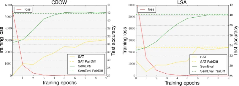
Figure 3: The training loss and test performance on SAT and SemEval benchmarks for relational embed-dings.
andq (on the right vertical axis) for the six word embeddings. In all cases, we see that as the training progresses, A goes to zero as predicted by Theorem 1 under regularisation. Moreover, we see that approximatelyp ≈ −q = cis reached for somec ∈ Rin all cases, which implies that P≈ −Q= cI, which is thePairDiffoperator. Among the six input word embeddings compared in Figure 1, HSC has the highest mean correlation (0.082), which implies that its dimensions are correlated more than in the other word embeddings. This is to be expected by design because a hierarchical structure is imposed on the dimensions of the word embedding during training. However, HSC embeddings also satisfy the
A ≈0andp ≈ −q =crequirements, as expected by thePairDiff. This result shows that the claim of Theorem 1 is empirically true even when the uncorrelation assumption is mildly violated.
4.3 Generalisation Performance on Analogy Detection
[image:9.595.98.501.312.458.2]To measure the generalisation capability of the learnt relational embeddings from BATS, we measure their performance on two other benchmark datasets: SAT Turney and Bigham (2003) and SemEval 2012-Task210. Note that we do notretrainA,P andQin (2) on SAT nor SemEval, but simply to use their values learnt from BATS because the purpose here to evaluate the generalisation of the learnt operator.
In SAT analogical questions, given a stem word-pair(a, b)with five candidate word-pairs(c, d), the task is to select the word-pair that is relationally similar to the the stem word-pair. The relational similar-ity between two word-pairs(a, b)and(c, d)is computed by the cosine similarity between the correspond-ing relational embeddcorrespond-ingsr(a,b) andr(c,d). The candidate word-pair that has the highest relational similarity with the stem word-pair is selected as the correct answer to a word analogy question. The re-ported accuracy is the ratio of the correctly answered questions to the total number of questions. On the other hand, SemEval dataset has 79 semantic relations, with each relation having ca. 41 word-pairs and four prototypical examples. The task is to assign a score for each word pair which is the average of the relational similarity between the given word-pair and prototypical word-pairs in a relation. Maximum difference scaling (MaxDiff) is used as the evaluation measure in this task.
Figure 3 shows the performance of the relational embeddings composed from 50-dimensional CBOW and LSA embeddings11. For CBOW, the level of performance reported byPairDiffon SAT and SemEval datasets are respectively35.16%and41.94%, and are shown by horizontal dashed lines. From Figure 3, we see that the training loss gradually decreases with the number of training epochs and the performance of the relational embeddings on SAT and SemEval datasets reach that of thePairDiffoperator. This result indicates that the relational embeddings learnt not only converge toPairDiffoperator on training data but also generalise to unseen relation types in SAT and SemEval test datasets.
5 Conclusion
This paper theoretically analyses the bilinear operator for representing relations between words using their embeddings. We showed that, if the word embeddings are standardised and uncorrelated, then the expected`2distance between analogous and non-analogous word-pairs is independent of bilinear terms,
and the relation embedding further simplifies to the popularPairDiffoperator under regularised settings. Among diverse methods for calculating word embeddings, we empirically show the uncorrelation in word embedding dimensions, which is one of the prerequisites for simplifying the bilinear operator to a linear one. Empirically, we supports the theoretical analysis by showing that when optimising a general bilinear formulation on a labeled word pair relational dataset, the solution converges to the simple linear form, and more specifically to the simplePairDiffformulation.
In this work, we model relations as vectors and we measure relational strength using Euclidean dis-tance. We are aware that there are many other relation representation methods and relational strength measurement methods besides what we have considered in the paper. Similar analysis can be conducted in follow-up work for different types of relation representations and strength measures. For instance, an interesting future research direction of this work is to extend the theoretical analysis to nonlinear relation composition operators, such as for nonlinear neural networks.
Acknowledgement
We gratefully acknowledge the support of NVIDIA Corporation with the donation of the Tesla K40 GPU used for this research.
References
William Blacoe and Mirella Lapata. 2012. A comparison of vector-based representations for semantic composition. InProc. of EMNLP. pages 546–556.
David M. Blei, Andrew Y. Ng, and Michael I. Jordan. 2003. Latent dirichlet allocation. Journal of Machine Learning Research3:993–1022.
10
https://sites.google.com/site/semeval2012task2/
Danushka Bollegala, Takanori Maehara, and Ken ichi Kawarabayashi. 2015a. Embedding semantic relationas into word representations. InProc. of IJCAI. pages 1222 – 1228.
Danushka Bollegala, Takanori Maehara, Yuichi Yoshida, and Ken ichi Kawarabayashi. 2015b. Learning word representations from relational graphs. InProc. of AAAI. pages 2146 – 2152.
Danushka Bollegala, Yutaka Matsuo, and Mitsuru Ishizuka. 2009. A relational model of semantic simi-larity between words using automatically extracted lexical pattern clusters from the web. InProc. of EMNLP. pages 803–812.
Antoine Bordes, Nicolas Usunier, Alberto Garcia-Durán, Jason Weston, and Oksana Yakhenko. 2013. Translating embeddings for modeling multi-relational data. InProc. of NIPS. pages 2787–2795.
Scott Deerwester, Susan T. Dumais, George W. Furnas, Thomas K. Landauer, and Richard Harshman. 1990. Indexing by latent semantic analysis.American Society for Information Science41(6):391–407.
Aleksandr Drozd, Anna Gladkova, and Satoshi Matsuoka. 2016. Word embeddings, analogies, and machine learning: Beyond king - man + woman = queen. InProc. of COLING. pages 3519–3530.
Nguyen Tuan Duc, Danushka Bollegala, and Mitsuru Ishizuka. 2010. Using relational similarity between word pairs for latent relational search on the web. InProc. of WI. pages 196–199.
John Duchi, Elad Hazan, and Yoram Singer. 2011. Adaptive subgradient methods for online learning and stochastic optimization. Journal of Machine Learning Research12:2121–2159.
Manaal Faruqui, Yulia Tsvetkov, Dani Yogatama, Chris Dyer, and Noah A. Smith. 2015. Sparse over-complete word vector representations. InProc. of ACL. pages 1491–1500.
Anna Gladkova, Aleksandr Drozd, and Satoshi Matsuoka. 2016. Analogy-based detection of morpholog-ical and semantic relations with word embeddings: what works and what doesn’t. InProc. of SRW@ HLT-NAACL. pages 8–15.
Shu Guo, Quan Wang, Lihong Wang, Bin Wang, and Li Guo. 2016. Jointly embedding knowledge graphs and logical rules. InProc. of EMNLP. pages 192–202.
Huda Hakami and Danushka Bollegala. 2017. Compositional approaches for representing relations be-tween words: A comparative study. Knowledge-Based Systems136:172–182.
Katsuhiko Hayashi and Masashi Shinbo. 2017. On the equivalence of holograpic and complex embed-dings for link prediction. InProc. of ACL. pages 554–559.
Sergey Ioffe and Christian Szegedy. 2015. Batch normalization: Accelerating deep network training by reducing internal covariate shift. InProc. of Machine Learning Research. pages 448–456.
David A. Jurgens, Saif Mohammad, Peter D. Turney, and Keith J. Holyoak. 2012. Semeval-2012 task 2: Measuring degrees of relational similarity. InProc. of *SEM. pages 356 – 364.
Omer Levy and Yoav Goldberg. 2014. Linguistic regularities in sparse and explicit word representations. InProc. of CoNLL. pages 171–180.
Omer Levy, Yoav Goldberg, and Ido Dagan. 2015. Improving distributional similarity with lessons learned from word embeddings. Transactions of Association for Computational Linguistics3:211– 225.
Tomas Mikolov, Kai Chen, and Jeffrey Dean. 2013a. Efficient estimation of word representation in vector space. InProc. of ICLR. pages 1–12.
Tomas Mikolov, Wen-tau Yih, and Geoffrey Zweig. 2013b. Linguistic regularities in continuous space word representations. InProc. of HLT-NAACL. pages 746–751.
Pasquale Minervini, Thomas Demeester, Tim Rocktäschel, and Sebastian Riedel. 2017. Adversarial sets for regularising neural link predictors. InProc. of UAI.
Maximilian Nickel, Kevin Murphy, Volker Tresp, and Evgeniy Gabrilovich. 2015. A review of relational machine learning for knowledge graphs. InProc. of the IEEE. 1, pages 11–33.
Maximilian Nickel, Lorenzo Rosasco, and Tomaso Poggio. 2016. Holographic embeddings of knowl-edge graphs. InProc. of AAAI. pages 1955–1961.
Maximilian Nickel, Volker Tresp, and Hans-Peter Kriegel. 2011. A three-way model for collective learning on multi-relational data. InProc. of ICML. pages 809–816.
Jeffrey Pennington, Richard Socher, and Christopher D Manning. 2014. Glove: Global vectors for word representation. InProc. of EMNLP. pages 1532–1543.
Tim Rocktäschel, Edward Grefenstette, Karl Moritz Hermann, Tomáš Koˇciský, and Phil Blunsom. 2016. Reasoning about entailment with neural attention. InProc. of ICLR.
Richard Socher, Danqi Chen, Christopher D Manning, and Andrew Ng. 2013. Reasoning with neural tensor networks for knowledge base completion. InProc. of NIPS. pages 926–934.
Théo Trouillon, Johannes Welbl, Sebastian Riedel, Éric Gaussier, and Guillaume Bouchard. 2016. Com-plex embeddings for simple link prediction. InProc. of ICML. pages 2071–2080.
Peter D Turney and Jeffrey Bigham. 2003. Combining independent modules to solve multiple-choice synonym and analogy. InProc. of RANLP. pages 482–489.
Peter D Turney and Michael L Littman. 2005. Corpus-based learning of analogies and semantic relations.
Machine Learning60(1):251–278.
Ekaterina Vylomova, Laura Rimell, Trevor Cohn, and Timothy Baldwin. 2016. Take and took, gaggle and goose, book and read: Evaluating the utility of vector differences for lexical relational learning. InProc. of ACL. pages 1671–1682.
Bishan Yang, Wen tau Yih, Xiadong He, Jianfeng Gao, and Li Deng. 2015. Embedding entities and relations for learning and inference in knowledge bases. InProc. of ICLR.
Wenpeng Yin and Hinrich Schütze. 2016. Learning meta-embeddings by using ensembles of embedding sets. InProc. of ACL. pages 1351–1360.