Outer Shells of Giant Planets
Thesis by
Junjun Liu
In Partial Fulfillment of the Requirements
for the Degree of
Doctor of Philosophy
1 8 9 1
C A L
I
F
O
RN
IA I
NS
TITUT E O F
T
E
C
H
N
O
L
O
G
Y
California Institute of Technology
Pasadena, California
2006
c
2006
Junjun Liu
Acknowledgements
It has been six years since I came to Caltech. I would like to express my gratitude to
all the people I met during this period. It has been a great journey.
First of all, I am indebted to my advisor, Dave Stevenson, who guided me into this
very interesting research area and has been extraordinarily supportive, inspiring and
patient all these years. Under his support, I had the opportunity to attend the GFD
summer school at Woods Hole in 2003 and Computational Fluid Mechanics summer
school at Helmholtz Institute in 2004. Both of them are very beneficial.
I would like to thank my advisor, Peter Goldreich, for his mentorship, guidance,
support and encouragement during my time at Caltech. His enthusiasm for science,
his positive attitude for life, and his belief that his students are capable of anything,
continue to inspire me.
I thank Andy Ingersoll for serving as my academic advisors through the years.
Thank Mark Richardson for introducing me interesting projects related with Mars
and many enjoyable conversations. Thank Yuk Yung for being my research advisor
for the first two years. I thank my thesis advisory committee - Andy Ingersoll, Peter
Goldreich, Tapio Schneider, Re’em Sari and Dave Stevenson for all the time and
thoughts they devoted to my TAC meetings.
I must thank Mike Black for resolving my numerous computer problems and am
very grateful for the care and support from the staff members, Leticia Calderon, Irma
Black, Nora Oshima, Loreta Young.
I thank Sarah Stewart, Ashwin Vasavada, Anthony Toigo, Zhiming Kuang, Lori
Fenton, Huiqun Wang, Antonin Bouchez, Shane Byrne, Xianglei Huang for help and
discussions. I also thank my officemates, Ah-San Wong, Mao-Chang Liang, Shabari
Basu, Jiafang Xiao, Dan Feldman, Nicholas Heavens and Michael Busch for many
enjoyable moments.
Yuanyuan and my brother Dixun for their unconditional support and
encourage-ments throughout the years of my education. I thank my daughter, Amy, for all the
joy and love she brings to my life. Finally, I am very grateful for the love and support
that my husband gave to me. Thank you, Lifeng, for being my husband and sharing
Abstract
This study of the interaction of magnetic field and flow in the outer shells of giant
planets consists of three parts.
Part one: The atmospheres of Jupiter and Saturn exhibit strong and stable zonal
winds. Busse suggested that they might be the surface expression of deep flows on
cylinders. However, the deep flow hypothesis experiences difficulty when account is
taken of the electrical conductivity of molecular hydrogen as measured in shockwave
experiments. The deep zonal flow of an electrically conducting fluid would produce
a toroidal magnetic field, an associated poloidal electrical current, and Ohmic
dissi-pation. In steady state, the total Ohmic dissipation cannot exceed the planet’s net
luminosity. If we assume that the observed zonal flow penetrates along cylinders
until it is truncated to (near) zero at some spherical radius, the upper bound on
Ohmic dissipation constrains this radius to be no smaller than 0.95 Jupiter radius
and 0.87 Saturn radius. The truncation of the cylindrical flow in the convective
enve-lope requires an appropriate force to break the Taylor-Proudman constraint. We have
been unable to identify any plausible candidate. Thus we conclude that deep-seated
cylindrical flows do not exist.
Part two: A fluid shell with sufficient electrical conductivity and azimuthal
veloc-ity shear outside of the dynamo generation region can attenuate the non-axisymmetric
component of the magnetic field. However, the interaction of the axisymmetric
com-ponent of the magnetic field and the zonal flow is able to reduce the magnitude of zonal
flow. The dimensionless number characterizing this reduction is the Chandrasekhar
number. The smaller Saturnian field may allow a larger velocity shear and a greater
attenuation of the non-axisymmetric field, thereby providing a possible explanation
for the nearly axisymmetric field.
Part three: Combining the study for the attenuation effect produced by the
we find the possible outer boundary of the dynamo generation zone is at 0.86 Jupiter
radius. The magnetic fields generated in the outer shell are dictated by a length scale
comparable to the scale height of electrical conductivity, which is much smaller than
Contents
Acknowledgements iii
Abstract v
1 Introduction 1
1.1 Main observation data . . . 1
1.2 Fundamental questions . . . 7
2 Electrical conductivity distribution in the interior of giant planets 9 2.1 Electrical conductivity distribution in the interior of Jupiter and Saturn 9 2.2 Electrical conductivity distribution in the interior of Uranus and Neptune 13 3 Impossibility of deep-seated zonal winds in Jupiter and Saturn 20 3.1 Abstract . . . 20
3.2 Introduction . . . 21
3.3 Order of magnitude analysis . . . 23
3.4 Detailed formulation . . . 24
3.5 Truncated zonal flows . . . 32
3.5.1 Total Ohmic dissipation . . . 32
3.5.2 Do deep-seated zonal flows exist? . . . 34
3.5.3 Maximum width of an equatorial jet . . . 43
3.6 Conclusion and discussion . . . 45
3.7 Appendix: choose the poloidal magnetic field models . . . 45
4.2 Order of magnitude analysis. . . 52
4.3 Detailed formulation . . . 55
4.4 Ohmic dissipation calculation . . . 64
5 Interaction of magnetic field and shear flow 67 5.1 Abstract . . . 67
5.2 Introduction . . . 67
5.3 Interaction of magnetic field with shear flow in a Cartesian geometry 68 5.3.1 Driving the flow by boundary stress: constant magnetic diffusivity 69 5.3.2 Driving the flow by boundary stress: variable magnetic diffusivity 72 5.3.3 Driving the flow with variable body forces: constant magnetic diffusivity . . . 73
5.4 Interaction of the magnetic field with the zonal flow in a spherical geometry . . . 78
5.5 Conclusion . . . 96
6 Attenuation of non-asymmetric magnetic field in the outer shell of giant planets 98 6.1 Abstract . . . 98
6.2 Introduction . . . 98
6.3 Attenuation of the non-axisymmetric magnetic field by the flow in a Cartesian geometry . . . 100
6.3.1 Attenuation produced by the specified shear flow: constant magnetic diffusivity . . . 100
6.3.2 Attenuation produced by the specified shear flow: variable mag-netic diffusivity . . . 106
6.3.3 Perturbation analysis: constant magnetic diffusivity . . . 108
6.3.4 Perturbation analysis: variable magnetic diffusivity . . . 112
6.4 The thin shell approximation and the boundary conditions . . . 112
7 Attenuation of temporal variations of magnetic field in the outer
region of Jupiter. 121
7.1 Abstract . . . 121
7.2 Introduction. . . 122
7.3 Comparing the electrical conductivity profiles of Jupiter and Earth . 125 7.4 Electromagnetic screening by the semi-conducting molecular hydrogen envelope . . . 125
7.5 Secular variation and the deduction of the dynamo generation size on Jupiter . . . 132
7.6 Attenuation of the magnetic field in the presence of the dynamo effect 133 7.6.1 No α-effect and no ω-effect . . . 136
7.6.2 Finiteα-effect and noω-effect: no time dependence . . . 138
7.6.3 Finiteα-effect and noω-effect: with time dependence. . . 140
7.6.4 No α-effect and finite ω-effect: no time dependence. . . 142
7.6.5 No α-effect and finite ω-effect: with time dependence . . . 146
7.6.6 Finiteα-effect and finite ω-effect: no time dependence. . . 147
7.6.7 Finiteα-effect and finite ω-effect: with time dependence . . . 148
7.7 α-ωdynamo generation in large electrical conductivity variation region: Cartesian geometry . . . 149
List of Figures
1.1 The relative size of four giant planets: Jupiter, Saturn, Uranus, and
Neptune. Adapted from Ingersoll (1990). . . 3
1.2 Zonal velocity versus latitude for all four giant planets. Velocity is
measured relative to the planetary interiors, whose rotations are
in-ferred from the periodic radio emissions. The measurements involve
tracking cloud image sequences. Adapted from Ingersoll et al. (1995). 6
2.1 Electrical conductivity inside giant planets: (a) Jupiter; (b) Saturn.
The solid line is the mean electrical conductivity of hydrogen and the
dashed lines bound the range of uncertainty in the measurements.
Ad-ditional uncertainties at the upper range of pressure arise from the
difficulty of associating T and p as measured in the experiment with
that inside the planet. Metallization is responsible for the plateau at
2×10⁵ S m−1 which occurs near 0.84 RJ and 0.63 RS. . . 12
2.2 Magnetic diffusivity λ in the interiors of Jupiter and Saturn. (a)
Jupiter; (b) Saturn. The magnetic diffusivity corresponding to the
metallic state of hydrogen is 4 m s−2. . . . 14
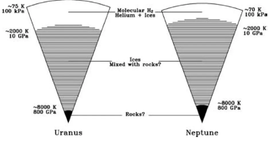
2.3 The interiors of Uranus and Neptune, adapted from Guillot (2005). . 15
2.4 Electrical conductivity versus shock pressure for planetary “ices”, adapted
from (Nellis et al., 1988). . . 17
2.5 Conductivity profiles in the interior of Uranus and Neptune based on
different “ice” mixing ratio in the outer “gas” envelope. (a) Uranus;
(b) Neptune. The solid line corresponds to no “ice” in the outer “gas”
envelope; the dash line represents 0.1% “ice” mixing ratio in the outer
envelope; the dash-dot line expresses 10% “ice” mixing ratio in the
3.1 Plots of U/uc versus (uB/uc)2 for different values of Γ at the radius
whereRm = 1. The solid line corresponds to Γ = 1, and the upper and
lower dash lines correspond to value of Γ≈20 and Γ≈ 2 appropriate
to Jupiter and Saturn. The diamond and circle correspond to values
of U and uB normalized by uc = (F/ρ)1/3, where ρ is evaluated at the
layer where Rm = 1. For Jupiter, U ∼100 m s−1, F ∼ 5 W m−2 and
Bp ∼10 G, so Γ∼20. For Saturn,U ∼400 m s−1,F ∼2 W m−2 and
Bp ∼1 G, so Γ∼2. . . 25
3.2 The current distribution inside the planets arising from the interaction
of a simple zonal flow and a purely axial dipole field. In this illustration,
the zonal flow goes to near zero just inside the dashed line. High
current density corresponds to closely spaced current flow lines, and the
conductivity is lower near the dashed line so that the Ohmic dissipation
is predominantly near the dashed line despite the volume filling nature
of the current. . . 31
3.3 We assume that the observed zonal flow penetrates to the interior along
cylinders until it is truncated at radiusr. The blue curve depicts the
to-tal Ohmic dissipation as a function of the fractional truncation radius.
The dashed curves indicate the range of uncertainty in the electrical
conductivity of hydrogen at a given radius. The horizontal green lines
marks to planet’s net luminosity, which is 3.35×10¹⁷ W for Jupiter
and 0.86×10¹⁷W for Saturn (Guillot et al., 2004). The maximum
pen-etration depth is determined by matching the total Ohmic dissipation
to the net luminosity. . . 33
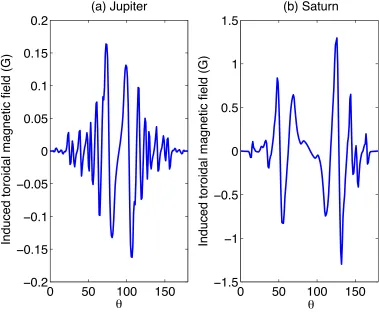
3.4 The induced toroidal magnetic field as a function of co-latitude at the
maximum penetration depth: (a) Jupiter, (b) Saturn. . . 34
3.5 The poloidal current density as a function of co-latitude at the
maxi-mum penetration depth: (a) Jupiter, (b) Saturn. . . 35
3.6 Total Ohmic dissipation rate verses jet half-width. The horizontal lines
3.7 This figure shows the comparison of the magnetic fields: the radial
com-ponent of the magnetic field versus the distance between the spacecraft
and the planets. The solid line is the magnetic field obtained from O6
model; the dash line is the calculated magnetic field with added
con-straints; and the dot indicates the closest approach of the spacecraft.
From this figure, we can see that the differences between two magnetic
field models are large (up to 0.5 G ∼ 50000 nT) close to the planets.
Far away from the planets, the differences are small and cannot be
detected. . . 49
4.1 This figure plots uU c
versus uB
uc
2
for different values of Γ at the
radius where Rm = 1. The solid line corresponds to Γ = 1. From top
to bottom, the dash lines correspond to value of Γ≈20, Γ≈ 2, Γ≈2.3
and Γ ≈ 0.2 appropriate to Jupiter, Saturn, Uranus and Neptune,
respectively. The diamond, star, circle and cross correspond to values
ofU anduB normalized byuc =
F ρ
1
3 whereρis evaluated at the layer
where Rm = 1. For Uranus, U ∼ 200 m s−1, F ∼ 0.06 W m−2 and
Bp ∼0.2 G, so Γ∼2.3. For Neptune,U ∼400 m s−1,F ∼ 0.45 W m−2
4.2 Here we assume that the observed zonal flow penetrates to the deep
interior along the cylinders. The flow has to be truncated at a
cer-tain radius to prevent production of excessive Ohmic dissipation. This
figure shows the total Ohmic dissipation versus the scaled truncation
radius: (a) Uranus; (b) Neptune. The solid blue curves show
calcu-lated total Ohmic dissipation if water-ice is confined in the “ice” layer;
the dash-line show total Ohmic dissipation if the mixing ratio of water
ice in the “gas” layer is 0.1%; the dot-line show total Ohmic
dissipa-tion if the mixing ratio of water ice in the “gas” layer is 10%. The
green horizontal line shows the planetary total luminosity, which is
0.034 ×10¹⁷ W for Uranus and 0.33×10¹⁷ W for Neptune (Guillot,
2005). The maximum penetration depth of the zonal flow is reached
when the total Ohmic dissipation produced by the flow matches the
planet’s net luminosity. For Uranus, the maximum penetration depth
increases from 0.80RU to 0.87RU as the mixing ratio of water ice
in-creases; For Neptune, the maximum penetration depth increases from
0.84RN to 0.85RN as the mixing ratio of water ice increases. . . 66
5.1 (a) The Cartesian geometry; (b) The magnetic field lines after
consid-ering interaction between magnetic field and shear flow. . . 69
5.2 The interaction of the magnetic field and the shear flow for constant
magnetic diffusivity. (a) Velocity versus height; (b) Induced horizontal
magnetic field versus height. The induced magnetic fieldB is scaled to
Rm/Q. For Q 1, the velocity amplitude reduction is proportional
to Q−1/2 and the maximum value of Rm/Q corresponds to balancing
the viscous and Maxwell stress, i.e.,B0B/μ0 ∼σin dimensional units.
The velocity shear is everywhere exponentially small except in the thin
5.3 Interaction of the magnetic field and the shear flow for various magnetic
diffusivities with different scale heights: λ = exp(βz), whereβ is taken
to be: 0.0,2.0,5.0,10.0. Here, Q= 103 and the induced magnetic field
is scaled to Q/Rm. (a) Velocity versus height; (b) Induced toroidal
magnetic field versus height. Reduction of the velocity is concentrated
in the region with large Q. . . 74
5.4 Interaction of magnetic field and shear flow if we drive the flow with
vertically varying body force(See equation (5.17)) for different Q. (a)
Velocity; (b) Induced magnetic field. B is scaled to Rm/Q. The
ve-locity shear is everywhere reduced by 1/Q relative to the zero field
case. . . 76
5.5 Flow velocity versus Chandrasekhar number for different driving forces.
Interaction of flow and magnetic field is characterized byQ. If the flow
is driven by boundary stress, the reduction of the velocity is
propor-tional toQ−1/2. If the flow is driven by body force, the reduction of the
velocity is proportional to Q−1. The fundamental difference between
these two cases is the role of boundary layers. . . 77
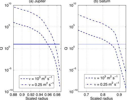
5.6 The Chandrasekhar number as a function of radius for Jupiter and
Sat-urn. (a) Jupiter; (b) SatSat-urn. If the viscosity is taken to be 0.25 m2s−1,
Qis larger than 10 below 0.92RJ for Jupiter and below 0.72RS for
Sat-urn. However, ifν ∼103 m s−2, the reduction of the velocity becomes
5.7 The time evolution of the azimuthal velocity for different Ekman
num-bers Eν at two different separated points in the interior of the fluid
domain far away from boundary. The spherical coordinate (r, θ) for
point one is (0.85R,71◦); and the spherical coordinate for point two is
(0.90R,127◦). (a) At point oneEν = 10−3; (b) At point twoEν = 10−3;
(c) At point oneEν = 10−4; (d) At point two Eν = 10−4. The Ekman
number Eν = ΩLν2 is the ratio of the rotational timescale to viscous
timescale. For Eν = 10−3, the viscous timescale is 103 times of the
rotation timescale. From figure (5.7a), we see that the system reaches
the steady state at 500 rotation timescale. Similarly, for Eν = 10−4,
the viscous timescale is 104times of the rotation timescale and the
sys-tem reaches the steady state at 5000 rotation timescale. The timescale
for reaching the steady state is proportional to inverse Ekman number
(T ∝ E1
ν). . . 86 5.8 The general solution of the velocity in steady state forEν = 10−3. (a)
The scaled zonal flow velocityUφ; (b) the meridional stream function.
Here the driving force is confined in the layer r > Ro, where Ro is
taken to be 0.95R. And, Γ = 1.0. The magnitude of the flow is not
zero outside of the surface layer despite the zero driving force in this
region. . . 88
5.9 The magnitude of the azimuthal flow along the rotation axis for
differ-ent cylindrical radius: s = 0.7R and s = 0.8R. Here Eν = 10−3 and
Γ = 1.0. . . 89
5.10 The ratio of the zonal flow on the surface to the penetrating flow for
differentEν. It is roughly independent ofEν providedEν is sufficiently
5.11 The solution with the deep-seated dipolar magnetic field and the
vari-able magnetic diffusivity distribution: λ = exp(βz). Here the
dimen-sionless numbers are taken to be: Γ ∼ 1.0, Λ ∼ 1.0, Eν ∼ 10−3 and
Eλ ∼ 10−3. (a) Ur; (b) Uθ; (c) Uφ; (d) meridional stream function
of velocity; (e) Br; (f) Bθ; (g) Bφ; (h) meridional stream function of
magnetic field. The interaction between the magnetic field and zonal
flow reduces the magnitude of the velocity shear and induces toroidal
magnetic field at the high electrical conducting region. . . 92
5.12 The magnitude of the zonal flow along the cylinders for different
cylin-drical radius. (a) Without the magnetic field. (b) with the magnetic
field, λ = λ0exp 20(r−ri), Λ = 0.2 and Eλ = 10−3. In both cases,
we take Eν = 10−3 and Γ = 1.0. For the case with magnetic field, the
curves for different cylindrical radiussnearly coincide at small z. This
demonstrates the reduction of velocity shear by the magnetic field in
the region with high electrical conductivity. The zonal flow at depth
in this case should be identified with the rotation of the core. . . 93
5.13 Relative velocity distribution in the equatorial plane. For the case with
the magnetic field,λ =λ0exp 20(r−ri), Λ = 0.2, Γ = 1.0, Eν = 10−3
and Eλ = 10−3. For the case without magnetic field Γ = 1.0,Eν = 10−3. 94
5.14 The relative velocity distribution in the equatorial plane for different
Λ. Here, λ = λ0exp 20(r−ri), Γ = 1.0, Eν = 10−3 and Eλ = 10−3.
For large Λ, the Lorentz force is strong and the velocity shear reduction
is more. . . 95
5.15 The relative velocity distribution in the equatorial plane as a function
of Chandrasekhar number for different Λ. Here: λ=λ0exp 20(r−ri),
Γ = 1.0, Eν = 10−3 and Eλ = 10−3. For large enough Q, the velocity
distribution is roughly proportional to the inverse of Chandrasekhar
6.1 The magnitude of the x-dependent magnetic field bz as a function of
heightz for differentRm. Here, thex-dependent vertical magnetic field
(bz = exp(ikx)) is imposed at the bottom boundary and the horizontal
wavenumber k is taken to be: k = 1. The attenuation effect is strong
for largeRm. . . 103
6.2 Magnetic field lines. (a) Without the flow; (b) with the flow fork = 1
and Rm = 103. With the flow, the magnetic field lines are dragged by
the flow and move together with the fluid in the high electric
conduct-ing region. . . 105
6.3 Demonstrate the mechanism of attenuating the x-dependent magnetic
field by the shear flow. . . 106
6.4 The attenuation of the x-dependent field by the specified shear flow
with variable magnetic diffusivity: λ=λ0exp(βz). Here k = 1, Rm =
103 and β is: β = 0.0; β = 5.0; β = 20.0. The attenuation effect is
concentrated in the region with low magnetic diffusivity. . . 107
6.5 Magnetic field line advected by the fluid for variable magnetic
diffusiv-ity: λ = exp(βz). Here Rm = 104, k = 1 and β = 10. The magnetic
field lines will only be advected by the flow in the region with low
magnetic diffusivity. . . 108
6.6 The relation between the physical attenuation factor and height for
different magnetic diffusivities: (a) drive the flow by boundary stress;
(b) drive the flow by variable body forces (see equation (6.25)). We
6.7 The attenuation for the tilted dipole produced by fluid motion in the
deep interior. (a) Jupiter; (b) Saturn. Here we assume that Jupiter and
Saturn have similar dipole tilt without being attenuated by the flow.
The solid line shows the scaled non-axisymmetric magnetic field
with-out being attenuated by the flow, where the magnetic field is scaled
by the maximum value of tilted dipole along the meridional
direc-tion. The circle corresponds to the external field after being
attenu-ated by the flow with U0 = 10−3 m s−1 and the hexagon represents
U0 = 2×10⁻³ m s−1, where U0 is the magnitude of the flow without
being reduced by the magnetic field. The flow has negligible effect in
reducing Jupiter’s outgoing tilted dipole. However, U0 = 10−3 m s−1
makes Saturn’s titled dipole 102 times smaller than that without the
attenuation; and U0 = 2×10⁻³ m s−1 makes it 104 times smaller. . . 118
6.8 Comparison between using constant B0 and B0(θ) as a function of θ.
(a)U0 = 0.02 cm s−1, (b) U0 = 0.05 cm s−1. The solid line corresponds
to the scaled non-axisymmetric magnetic field without attenuated by
the flow. The circle corresponds to external magnetic field with
con-stant B0 and the hexagon represents to external magnetic field with
B0 as a function of θ. B0(θ) is taken to be the observed value. . . 119
7.1 Comparison between the conductivity profile of Jupiter to that of the
earth. The dash line expresses the conductivity profile of Earth, and
the solid line is the conductivity profile of Jupiter. . . 126
7.2 The attenuation effect produced by the semi-conducting layer. The
outer boundary of the dynamo generation region is taken to be 0.84RJ,
which corresponds to the electrical conductivity 2×10⁵ S m−1. (a)
The absolute value of the attenuation factor; (b) the phase shift of the
attenuation factor. . . 131
7.4 The absolute value of the reduction factor versus the period of the
magnetic field for the different assumption of the magnitude of the
Chapter 1
Introduction
Jupiter, Saturn, Uranus and Neptune are giant planets in our solar system. They
are made of a fluid envelope and possibly a small dense central core. For Jupiter
and Saturn, the fluid envelope is composed of hydrogen (∼92% atomic) and helium
(∼8%), and a small amount of heavy elements. For Uranus and Neptune, the fluid
envelope may be divided into two layers: the gas layer, which is mainly composed
of hydrogen and helium; and the ice layer, which is primarily made of “ices”
in-cluding molecular species such as water, methane, and ammonia in the fluid state. In
contrast to the terrestrial planets, the viscosity can be neglected in the fluid envelope.
The interiors of giant planets are expected to evolve with time from a high entropy,
hot initial state to a low entropy, cold degenerate state. They have hot interiors and
emit more energy than they absorb from the Sun (Guillot, 2005). The heat source
is mainly gravitational-either in the form of primordial heat generated during the
collapse leading to planetary formation, or in the form of outgoing differentiation of
heavy material from light material. The heat from the interior can be transported
through diffusion, radiation and convection. Since the opacity is too high for effective
radiative transfer and the thermal diffusivity is too small for effective diffusion,
ther-mal convection was identified to be the main transport mechanism (Hubbard, 1968).
Furthermore, the presence of alkali metals ensures convective interiors (Burrows et al.,
2000; Guillot et al., 2004; Guillot, 2005).
1.1
Main observation data
Table 1.1 indicates the characteristics of the gravitational fields and orbits for giant
planets. The masses of the giant planets can be determined from their external
with great accuracy: 317.834, 95.161, 14.538, 17.148 times the mass of the Earth
for Jupiter, Saturn, Uranus, and Neptune, respectively (Campbell & Synnott, 1985;
Campbell & Anderson, 1989; Anderson et al., 1987; Tyler et al., 1989). These four
giant planets comprise about 99.5% of the planetary mass in our solar system.
The radii of the giant planets corresponding to the 1 bar pressure level are obtained
by radio occultation experiments (Lindal et al., 1981, 1985; Lindal, 1992). Figure (1.1)
shows their relative sizes. All four giant planets are relatively fast rotators, with
peri-ods of approximately 10 hours for Jupiter and Saturn and approximately 17 hours for
Uranus and Neptune. For Jupiter, Uranus and Neptune, the rotation rate is taken
to be the magnetic field rotation rate, which is tied to the deep interior (Dessler,
1983; Davies et al., 1986; Warwick et al., 1986, 1989). However, Saturn’s observed
magnetic field is nearly axisymmetric, which prevents a rotation rate determination
by Pioneer 11. The flyby of Voyager I and II detected period Saturn’s kilometric
radio emission (SKR), which had led to a magnetically defined rotation period for
that planet (Desch & Kaiser, 1981). Since then the SKR period has varied by 1%
(Galopeau & Lecacheux, 2000) and is currently 10 hour 45 min 45 s (Gurnett et al.,
2005). It is unclear that SKR emission really represents Saturn’s rotation and the
reason for the period drift between 1980-1981 and 1994-2000 is unknown.
The mean density ¯ρlisted in table 1.1 provides an important constraint on internal
composition. The ¯ρ values for Jupiter and Saturn imply that hydrogen is the major
constituent, whereas Uranus and Neptune require more dense constituents.
Table 1.2 shows the energy balance as determined from Voyager IRIS data (Pearl
& Conrath, 1991). Jupiter, Saturn and Neptune are observed to emit significantly
more energy than they receive from the Sun (see Table 1.2). The case of Uranus
is less clear. Its intrinsic heat flux Fint is one to two orders of magnitude smaller
than that of the other giant planets. However, detailed modeling by a
sug-Figure 1.1 The relative size of four giant planets: Jupiter, Saturn, Uranus, and Nep-tune. Adapted from Ingersoll (1990).
Table 1.1. Characteristics of the gravity fields and orbits.
Parameter, symbol Jupiter Saturn Uranus Neptune
Mass,M(M⊕) 317.834 a 95.161 b 14.538c 17.148 d Equatorial radius, re
103 km 71.4 e 60.3 f 25.6g 24.8 g
Equatorial gravity, g( m s−1) 22.9 9.1 8.8 11.1 Mean density, ¯ρ( g cm−3) 1.3275 0.6880 1.2704 1.6377 Rotation frequency, Ω(10−4 s) 3.57297(41) h 3.83577(47) h 6.206(4)i 5.800(20) j
Orbital period, 2πΩ−o1 (year) 11.9 29.5 84.0 164.8
aCampbell & Synott, 1995
bCampbell & Anderson, 1989
cAnderson et al., 1987
dTyler et al., 1989
eLindal et al., 1981
fLindal et al., 1985
gLindal, 1992
hDavis et al., 1986
iWarwick et al., 1986
Table 1.2. Energy balance as determined from Voyager IRIS dataa.
Parameter, symbol Jupiter Saturn Uranus Neptune
Absorbed power [1023 erg s−1] 50.14(248) 11.14(50) 0.526(37) 0.204(19)
Emitted power [1023 erg s−1] 83.65(84) 19.77(32) 0.560(11) 0.534(29) Intrinsic power [1023 erg s−1] 33.5(26) 8.63(60) 0.034(38) 0.330(35) Intrinsic flux [ erg s−1 cm−2] 5440.(430) 2010.(140) 42.(47) 433.(36)
Effective temperature [ K] 124.4(3) 95.0(4) 59.1(3) 59.3(8) 1-bar temperatureb[ K] 165.(5) 135.(5) 76.(2) 72.(2)
aPearl & Conrath, 1991
bLindal, 1992
gests thatFint≥60 erg cm−2 s−1 (Marley & McKay, 1999). Following this result, all
four giant planets can be said to emit more energy than they receive from the Sun.
In the outer shells of giant planets, hydrogen (the dominant component) is
su-percritical, which indicates that there is no gas-liquid or gas-solid phase transition at
that region. These planets have bottomless atmospheres, which is fundamentally
dif-ferent from terrestrial planets. The circulation in the atmosphere is powered by solar
energy and internal energy left over from the formation of solar system. The observed
zonal winds are very strong and stable. They reache ∼ 100 m s−1 and ∼ 400 m s−1
in the equatorial region of Jupiter and Saturn respectively. Uranus’ zonal winds peak
in the mid-latitude reaching ∼ 200 m s−1. Neptune’s zonal flows peak in equatorial
region reaching∼400 m s−1 (Ingersoll et al., 1995). The profiles of zonal (azimuthal)
velocity versus latitude for all four giant planets are shown in figure (1.2).
Prograde equatorial jets have been observed for Jupiter and Saturn’s equatorial
re-gion, whereas Uranus and Neptune have retrograde equatorial jets. At mid-latitudes,
Jupiter’s jets exhibit alternating prograde and retrograde bands, whereas Saturn’s
major jets are all prograde. Uranus and Neptune have smoother profiles than Jupiter
For the deep winds, the Galileo probe descended at 7.4◦N on Jupiter and
mea-sured the speed from 0.4 to 22 bars. At the 0.4 bar level, the measured wind speed is
90 m s−1 (Atkinson et al., 1997, 1998). The velocity of winds increased with depth to
180 m s−1 and remained nearly constant until 22 bars. Although these measurements
indicate that winds increase below the cloud level, they are not deep enough to reveal
the vertical structure except for less than 1% of the planetary radius.
Giant planets have strong and complex magnetic fields. The observed dipole
component of the surface field for Jupiter is about 4.2 G; and it is about 0.2 G for
Saturn, Uranus and Neptune. The observed magnetic field is predominantly dipolar
for Jupiter and Saturn. The tilt of the dipole relative to the rotation axis is on the
order of 10◦ for Jupiter and near zero for Saturn. For Uranus and Neptune, the field
is about equally dipole and quadrupole and the tilt of the dipole is 40◦-60◦, which
demonstrates large variation on the surface (Connerney, 1993).
As in Earth, the observed magnetic field is generated in the high electrical
con-ducting region. In the interiors of giant planets, the pressure and temperature increase
with depth. Shockwave experiments have measured the electrical conductivity of
hy-drogen from 0.93 Mbar to 1.8 Mbar and an estimated temperature at 3000 Kelvin,
representative of conditions inside Jupiter and Saturn (Nellis et al., 1996). Since
hydrogen is expected to be in thermal equilibrium in this measurement, the results
are applicable to the planetary interior. This experiment suggests that hydrogen
undergoes a continuous transition from semi-conducting molecular state to metallic
state as the pressure increases. The electrical conductivity increases exponentially
to 2.0×10⁵ S m−1 at 1.4Mbar where hydrogen becomes metallic. This
conductiv-ity of metallic hydrogen is one to two orders of magnitude lower than that of good
metals (such as copper) at room temperature, and is about the lowest possible value
for a metal. For Uranus and Neptune, measurements were made of electrical
and “synthetic Uranus” at shock pressures and temperatures up to 75 GPa and
5000 K. The electrical conductivity increases with depth and reaches a constant
value of 2×10³ S m−1 above 40 GPa (Nellis et al., 1988).
For Jupiter, Uranus and Neptune, the magnitude of the wind speeds is
deter-mined relative to the planetary magnetic field, which is called System III (Dessler,
1983; Davies et al., 1986; Warwick et al., 1986, 1989). In the deep interior, the
con-ductivity of metallic hydrogen is high, which implies the magnetic diffusivity is low.
The magnetic field lines are fixed in the fluid and advected by the flow. The
rel-ative velocity between the magnetic field and the fluid is small, i.e., the magnetic
field is nearly in a solid rotating state in this region. Comparing the measurements
from Voyager and Galileo, the dipole tilt increases 0.3 deg and the magnitude of the
dipole moment increases up to 1.5% over the period from 1975 to 2000 (Russell et
al., 2001ab), inferring an upper bound for the relative velocity between the
mag-netic field and the flow in the deep interior to be about 0.1 cm s−1 (Guillot et al.,
2004). For Saturn, the magnitude of the wind speeds is determined relative to SKR
since Saturn’s observed magnetic field is nearly axisymmetric (Desch & Kaiser, 1981).
1.2
Fundamental questions
How deep do the zonal winds extend? What are the possible generation mechanisms
for the zonal winds? If the observed flow penetrates to the deep interior along the
Taylor-Proudman cylinders as suggested by Busse (1976, 1983, 1994), the azimuthal
flow will interact with the pre-existing poloidal magnetic field, produce toroidal
mag-netic field and the associated Ohmic dissipation. The total Ohmic dissipation cannot
be larger than the planetary net luminosity, which gives a constraint for the maximum
penetration depth of the zonal flow. The zonal wind has to be truncated before
reach-ing the maximum penetration depth to avoid producreach-ing excessive Ohmic dissipation.
col-umn, we give a constraint for the depth of the zonal wind, as well as the generation
mechanism.
On the other hand, the deeper and higher conductivity region would force the
magnetic field lines to be almost fixed in the fluid and advected with the flow. The
relative velocity between the fluid and the field is small. The magnetic field behaves
like elastic strings. A large velocity between the fluid and magnetic field is not allowed
since it produces large elastic stress acting on the fluid and reduces the velocity shear.
Also, the velocity outside of the dynamo generation region is able to attenuate the
temporal variation of the outgoing magnetic field, as well as the non-axisymmetric
magnetic field. So, the following competing effects exist: The magnetic field is able
to reduce the shear flow; and the shear flow is able to attenuate the temporal
vari-ation of the outgoing magnetic field and the non-axisymmetric magnetic field. Can
the magnetically limited shear flow significantly attenuate the temporal variation of
magnetic field and the non-axisymmetric magnetic field?
In this thesis, we explore the interaction of magnetic field and flow in the outer
shells of giant planets. This study is motivated by the following fundamental
ques-tions:
1. Does the observed zonal flow penetrate to the deep interior along Taylor
cylin-ders?
2. How does the interaction between the magnetic field and zonal flow change the
Taylor cylinders?
3. Does the zonal flow attenuate the non-axisymmetric magnetic field? How?
4. Does the zonal flow attenuate the temporal variation of the outgoing magnetic
field? How?
5. What are the characteristics of dynamo generation in a region with rapidly
Chapter 2
Electrical conductivity
distribution in the interior of giant planets
2.1
Electrical conductivity distribution in the
in-terior of Jupiter and Saturn
The electrical conductivity in the interiors of Jupiter and Saturn is due mainly to
hydrogen. Near their surfaces it might be significantly enhanced relative to pure
hydrogen by heavier elements because they are more readily ionized. Helium is
unim-portant due to its high ionization energy.
Condensed molecular hydrogen is a wide band-gap insulator at room temperature
and pressure, with a band gap, Eg, of about 15 eV, corresponding to the ionization
energy of the hydrogen molecule. As the pressure increases, this gap is expected to
diminish and finally close to zero, resulting in an insulator-to-metal transition. In
ex-periments, this transition appears to be gradual. As the energy gap closes, hydrogen
molecules begin to dissociate to monatomic hydrogen and electrons start to be
delo-calized from H+2 ions (Nellis et al., 1996; Weir et al., 1996). The insulator-to-metal
transition is expected to occur even though the hydrogen molecules have not been
fully pressure-dissociated. At much higher pressure and temperature, molecular
dis-sociation becomes complete and it is presumed that pure monatomic hydrogen forms
a metallic Coulomb plasma (Stevenson & Ashcroft, 1974; Hubbard et al., 1997), but
this is irrelevant to our analysis.
The conductivity of hydrogen has been measured in reverberating shockwave
and from 0.1−0.2 Mbar (Nellis et al., 1992).1 In these experiments, hydrogen is
in thermal equilibrium at pressures and temperatures similar to those in the
inte-riors of giant planets. From 0.93 to 1.8 Mbar, the measured electrical conductivity
of hydrogen increases four orders of magnitude. Above 1.4 Mbar up to 1.8 Mbar,
the conductivity is constant at 2×10⁵ S m−1, similar to that of liquid Cs and Rb
at 2000 K and two orders of magnitude lower than that of a good metal (e.g., Cu)
at room temperature. The constant conductivity suggests that the energy gap has
been thermally smeared out (Weir et al., 1996). Temperatures of shock-compressed
liquid hydrogen have been measured optically in separate experiments (Nellis et al.,
1995; Holmes et al., 1995). At the highest obtained pressure of 0.83 Mbar, the
mea-sured temperature of 5200 K falls below that predicted for pure molecular hydrogen.
This is due to the dissociation of molecular hydrogen and enables us to estimate the
fractional dissociation as a function of pressure. At 1.4 Mbar and 3000 K, the
dis-sociation fraction is ∼ 5%. Thus metallization of hydrogen occurs in the diatomic
molecular phase and is caused by electrons delocalized from H+2 ions (Nellis et al.,
1996; Ashcroft, 1968).
The electrical conductivity of a semiconductor can be expressed in the form:
σ =σ0(ρ) exp
−Eg(ρ)
2KBT
, (2.1)
where σ is electrical conductivity, Eg(ρ) is the energy of the density dependent
mo-bility gap, KB is Boltzmann constant, T is the temperature, and exp (−Eg/2KBT)
expresses the fractional occupancy of the current carrying states.
Between 0.2 Mbar and 1.8 Mbar, we adopt the electrical conductivity profile
inter-polated by Nellis et al. (1996) based on the experimental data. The relation between
the energy gap and volume density is taken to be Eg = 20.3−64.7ρ, where Eg is in
eV, ρ in mol cm−3, and σ
Nellis et al. (1996) calculate the conductivity profile along an isentrope of hydrogen
starting from conditions deduced from observations of Jupiter’s atmosphere, namely
T = 165 K andp= 1 bar. This isentrope has the same entropy as one that has
com-monly been used to construct interior models of Jupiter (Guillot, 1999). However, it
has a lower T for p > 0.4 Mbar because the one used in these models neglects the
latent heat of hydrogen molecule dissociation (Nellis et al., 1995).2 For consistency,
we use the relation between conductivity and pressure obtained by Nellis et al. (1996).
For somep, theσbased on the commonly used isentrope (Guillot, 1999) is about one
order of magnitude different near the metallic conducting region and this difference
diminishes towards the surface.
Eg(ρ) has also been measured in shockwave experiments from 0.1 to 0.2 Mbar
(Nellis et al., 1992). We can interpolate between these measurements of Eg(ρ) and
its value at ambient pressure and temperature using σ0 = 0.5×10⁸ S m−1 (which
gives the smooth connection of the conductivity measured in two pressure ranges) to
extend the conductivity of hydrogen to the surface pressure level.
Based on the p(r) from interior models of Jupiter and Saturn (Guillot, 1999) and
σ(p) from Nellis et al. (1996), we obtain the electrical conductivity of hydrogen as a
function of radius (see figure 2.1). A clear signature of a smooth transition from the
semi-conducting to metallic state (withσ = 2×10⁵ S m−1) is observed at 0.84R
J and
0.63RS.
Figure (2.1) may underestimate the electrical conductivity at low pressure because
it neglects the contribution from impurities. The electrical conductivity is
propor-tional to the total number density of electrical charge carriers: σ∝ne, which includes
0.8 0.85 0.9 0.95 1 10−12
10−10 10−8 10−6 10−4 10−2 100 102 104 106
Scaled radius
Eletical conductivity (S/m)
(a) Jupiter
0.5 0.6 0.7 0.8 0.9 1 10−12
10−10 10−8 10−6 10−4 10−2 100 102 104 106
Scaled radius
Eletical conductivity (S/m)
[image:31.612.138.504.195.492.2](b) Saturn
Figure 2.1 Electrical conductivity inside giant planets: (a) Jupiter; (b) Saturn. The solid line is the mean electrical conductivity of hydrogen and the dashed lines bound the range of uncertainty in the measurements. Additional uncertainties at the upper range of pressure arise from the difficulty of associating T and p as measured in the experiment with that inside the planet. Metallization is responsible for the plateau at 2×10⁵ S m−1 which occurs near 0.84R
a contribution from impurities x in addition to that from hydrogen:
ne =nH2exp
− Eg
2KBT
+
x
nxexp
− Ex
2KBT
, (2.2)
where nx and Ex express the number density of the electrons and the energy gap
due to an impurity. Alkali metals are sources of small band gap impurities. They
may also contribute to the radiative opacity thus insuring adiabaticity (Guillot et al.,
2004; Guillot, 2005). The mixing ratio of an alkali metal in the interior of a giant
planet is presumably similar to that determined from its cosmic abundance. With
these abundances, a band gap of a few electron volts would lead to a conductivity of
10−6 ∼10−4 S m−1 atT ∼1000 K, significantly above the value due to hydrogen.
In magnetohydrodynamics it is conventional to characterize the electrical
conduc-tivity σ in terms of the magnetic diffusivity λ = (μ0σ)−1, where μ0 is the magnetic
permeability. Figure (2.1) shows that the electrical conductivity of hydrogen
de-creases exponentially outward from the metallic conducting region. Therefore, the
magnetic diffusivity increases exponentially outward (see fig. 2.2) We will make use
of the scale height of magnetic diffusivity,
Hλ(r) =
λ(r)
dλ(r)/dr. (2.3)
2.2
Electrical conductivity distribution in the
in-terior of Uranus and Neptune
Estimations based on mass, radius, rotational rate, and gravity field of the planets
indicate that Uranus and Neptune have similar internal structures (Stevenson, 1982).
0.8 0.9 1 100
102 104 106 108 1010 1012 1014
Scaled radius
Magnetic diffusivity (m
2 s
−
1 )
(a) Jupiter
0.6 0.8 1
100 102 104 106 108 1010 1012 1014
Scaled radius
Magnetic diffusivity (m
2 s
−
1 )
[image:33.612.128.503.214.515.2](b) Saturn
Figure 2.3 The interiors of Uranus and Neptune, adapted from Guillot (2005).
core region lie close to that of ices (a mixture initially composed of H2O, CH4 and
N H3, which rapidly becomes an ionic fluid of uncertain chemical composition in the
planetary interior), except in the outermost layers, which have a density closer to that
of hydrogen and helium (Marley et al., 1995; Podolak et al., 2000). As illustrated in
Figure (2.3), a three-layer model of Uranus and Neptune consists of a central rock
core (magnesium-silicate and iron material), an ice layer, and a hydrogen-helium gas
envelope (Podolak et al., 1991; Hubbard et al., 1995).
To interpret the origin of the planetary magnetic field, measurements were made
of electrical conductivity and equation of state of the planetary “ices”: water,
am-monia, methane and “synthetic Uranus” at shock pressures and temperatures up to
75 Gpa and 5000 K (See fig. 2.4). The electrical conductivities of the planetary
“ices” all approach a constant value of 2000 S m−1 above 40 GPa. This upper limit
is only weakly sensitive to chemical species (Nellis et al., 1988). The high electrical
ioniza-tion. Above 20 GPa, water has been said to be totally ionized intoOH−1 and H 3O+.
Using a classical conductivity model and a mean free path of a molecular dimension,
the degree of dissociation of water has been estimated to be between 10% and 100%
above 20 GPa and 1200 K (Nellis et al., 1988).
We calculate the electrical conductivity for the interior of Uranus and Neptune
with a three-layer model (Hubbard et al., 1991). In this model, both Uranus and
Neptune are assumed to have a central rocky core with chondritic bulk proportions of
iron, oxygen, magnesium, and silicon. The intermediate envelope is composed of “ice”,
which “ice” is defined as a mixture of the molecules H2O, CH4, and N H3 in solar
proportions, and almost certainly in liquid phase because of elevated temperatures.
The outer shell is mainly made of hydrogen and taken to have a pressure density
relation appropriate to solar composition (or to solar composition with a small density
enhancement) and at constant specific entropy with the entropy fixed to the value
near 1-bar pressure at a temperature of 70 K. The transition radius between the
intermediate “ice” layer and the outer gas envelope is taken to be ∼ 0.8 Uranus
radius and ∼ 0.84 Neptune radius, respectively. In the intermediate “ice” layer,
which ranges from ∼ 0.3Mbar at ∼ 3000 K to ∼ 6Mbar at ∼ 7000 K, we use the
conductivity profile for water ice to approximately express the planetary conductivity
profile. With p(r) in Hubbard’s model (Hubbard et al., 1991) and the conductivity
profile of water iceσ(p) (Mitchell and Nellis, 1982; Nellis et al., 1988), we obtainσ(r)
for the ice in Uranus and Neptune respectively. The outer “gas” envelope is mainly
composed of hydrogen with a small amount of heavy elements. We mainly consider
the influence of hydrogen and water ice to the total conductivity. In this case, the
number density of the electrical charge carriersne can be written as
ne =nH2exp
−(Eg)H2
2KBT
+nH2Oexp
−(Eg)H2O
2KBT
. (2.4)
Since the electrical conductivity is proportional to the number density of electrical
et al., 1996), and σ(p) for water ice (Mitchell and Nellis, 1982; Nellis et al., 1988).
The conductivity profile σ(r) largely depends on the mixing ratio of water ice in the
outer “gas” envelope. In figure (2.5), we demonstrate the conductivity profiles for a
different assumption of the water ice mixing ratio range from 0% to 10%. If “ice”
is present at 10% mixing ratio in the outer envelope, the electrical conductivity of
material in the outer envelope is significantly increased by many orders of magnitude.
On the other hand, the mixing of hydrogen in the intermediate “ice” layer can
significantly increase the electrical conductivity up to 100 times larger. In this thesis,
we are mainly interested in the conductivity profile in the outer envelope of the
planets. Therefore, we will not investigate the enhancement of electrical conductivity
0.7
0.75
0.8
0.85
10
−1510
−1010
−510
0scaled radius
conductivity (S m
−
1
)
(a). Uranus
0 %
0.1 %
10 %
0.75
0.8
0.85
0.9
10
−1510
−1010
−510
0scaled radius
conductivity (S m
−
1
)
(b). Neptune
[image:38.612.92.534.156.535.2]0 %
0.1 %
10 %
Chapter 3
Impossibility of deep-seated
zonal winds in Jupiter and Saturn
3.1
Abstract
The atmospheres of Jupiter and Saturn exhibit strong (∼100 m s−1) and stable (over
decadal time scales) zonal winds. Busse (1976, 1983, 1994) suggested that they might
be the surface expression of deep flows on cylinders. Wind velocities deduced from
the motion of the Galileo probe as it descended through Jupiter’s atmosphere offer
some support for Busse’s suggestion. However, the deep flow hypothesis experiences
difficulty when account is taken of the electrical conductivity of molecular hydrogen as
measured in shockwave experiments. The deep zonal flow of an electrically conducting
fluid would produce a toroidal magnetic field, an associated poloidal electrical current,
and Ohmic dissipation. In steady state, the total Ohmic dissipation cannot exceed the
planet’s net luminosity. If we assume that the observed zonal flow penetrates along
cylinders until it is truncated to (near) zero at some spherical radius, the upper bound
on Ohmic dissipation constrains this radius to be no smaller than 0.95 of Jupiter’s
radius and 0.86 of Saturn’s radius. At these radii, the electrical conductivity of
hydrogen is about 0.1 S m−1. The truncation of the cylindrical flow in the convective
envelope requires an appropriate force to break the Taylor-Proudman constraint. We
have been unable to identify any plausible candidate. The Lorentz force is much
too weak. Although we lack a convincing model for turbulent convection, order of
magnitude considerations suggest that both divergence of the Reynolds stress and the
buoyancy force are also inadequate. Thus we conclude that deep-seated cylindrical
flows do not exist. However, equatorial jets could maintain constant velocities on
cylinders through the planet provided their half-widths were no greater than ≈ 21◦
3.2
Introduction
Jupiter and Saturn are composed primarily of hydrogen and helium with small
ad-ditions of heavier elements. Their atmospheres exhibit strong, stable zonal winds
composed of multiple jets associated with azimuthal cloud bands (Ingersoll, 1990).
Zonal winds peak in the equatorial region reaching ∼ 100 m s−1 on Jupiter and
∼400 m s−1 on Saturn.1 The latitudes of Jupiter’s jets have not changed for at least 80 years (Smith & Hunt, 1976) and their velocities have been constant within 10%
over 25 years (Porco et al., 2003).
The depth of the zonal winds is unknown. Both deep and shallow flow models
have been proposed. Wind speeds measured by the Galileo probe at 7.4◦N on Jupiter
increased from 90 m s−1 at 0.4 bar to 180 m s−1 at∼ 5 bar and then remain nearly
constant until 22 bar (Atkinson et al., 1997, 1998). It is important to bear in mind
that these measurements only sample the winds in the outer 1% of the planet’s radius.
Where the electrical conductivity is high, the magnetic field lines are frozen into the
fluid. Thus winds in these regions would cause changes in the external magnetic field.
By comparing Galileo and Pioneer/Voyager data, Russell et al.(2001a,b) find that
increases of 0.3 deg in the dipole tilt and 1.5% in the dipole moment may have taken
place between 1975 and 2000. The former could be accounted for by meridional flow
speeds on the order of 0.1 cm s−1 in the deep interior of Jupiter (Guillot et al., 2004).
Busse (Busse, 1976, 1983, 1994) advocates deep flows. Since Jupiter’s interior is
believed to be convective (Hubbard, 1968; Guillot et al., 2004), he asserts that the
Taylor-Proudman theorem (Taylor, 1923) applies throughout the molecular hydrogen
envelope. It follows that the zonal flows extend along cylinders centered on, and
parallel to, the rotation axis, which terminates at the outer boundary of the metallic
hydrogen core. Hydrogen is assumed to undergo a first order phase transition at
the core-envelope boundary at which it abruptly changes from electrically insulating
to electrically conducting.2 In Busse’s model, the magnetic field is generated in the
metallic core and passes through the molecular envelope without interaction. But
data from shock wave experiments shows that hydrogen undergoes a continuous
tran-sition from a semi-conducting molecular state to a highly conducting metallic state
as the pressure increases. This contradicts the assumption of a first order phase
tran-sition at the core-envelope boundary.
Recently, a modified deep flow model for Jovian zonal flows has been proposed
based on simulations of convection in a thin shell with a lower boundary near 0.9RJ
(Aurnou & Heimpel, 2004; Heimpel et al., 2005). The physical meaning of the lower
boundary in the modified deep flow model is obscure. Hydrogen cannot undergo a
phase change at that radius (Guillot et al., 2004). So how might the Taylor-Proudman
constraint be violated in order to reduce the zonal flow to a near zero value below
that boundary? We demonstrate later that the Lorentz force is much too weak to
accomplish this.
In shallow flow models, the observed high-speed flow is confined to a thin,
baro-clinic layer near the cloud level; the interior flow is much slower. Even if the high
velocity flow is confined to a shallow layer, its forcing may occur at depth. For
ex-ample, if the flow were to arise from a process that conserved angular momentum
per unit volume, ρU would be approximately conserved, where ρ is the density and
U is the magnitude of the flow velocity. Since the density in the interior is several
orders of magnitudes larger than that near the surface, the flow velocity could then
be much greater near the surface. On the other hand, the observed zonal flow might
be generated by shallow forcing due to the turbulence injected at the cloud level by
moist convection, differential latitudinal solar heating, latent heat release from
con-densation of water, or other weather layer processes (Vasavada & Showman, 2005).
From the thermal wind equation, a latitudinal temperature gradient of about 5-10K
2In earlier models, this radius was estimated to be about 0.75R
J for Jupiter and 0.55RS for
across a few pressure scale heights below the cloud level would cause substantial
ver-tical shear, which makes the flow velocity much greater near the surface than deeper
down (Ingersoll & Cuzzi, 1969; Ingersoll et al., 1984; Vasavada & Showman, 2005).
In this paper, we examine the consequences of assuming a deep azimuthal flow
consistent with the Taylor-Proudman theorem for an adiabatic interior. We calculate
the total Ohmic dissipation associated with the flow and compare it to the planet’s
net luminosity. This constrains the depth to which the flow can extend. We consider
two flow patterns, one in which the flow is truncated to zero at a spherical radius,
and the other in which the flow is constant along the entire cylinder but confined to
an equatorial jet.
3.3
Order of magnitude analysis
We use order of magnitude analysis to illustrate the relation between the total Ohmic
dissipation and the planetary net luminosity. This clarifies the regime in which Jupiter
and Saturn operate. Three characteristic velocities are: U, the magnitude of the
ob-served zonal flow; uc = (F/ρ) 1/3
, a characteristic convective velocity based on the
heat flux,F, and density,ρ; uB=
B2
p/μ0ρ
1/2
, a characteristic Alfven velocity based
on the magnitude of the observed poloidal magnetic field, Bp. We note that the
defi-nition of the convective velocity does not take into account the influences of rotation
and magnetic field.
Consider a zonal flow of amplitude U that extends to a depth d∗ = R−r∗ and
weakens below. Define the magnetic Reynolds numberRm =U Hλ/λ. The magnitude
of the electrical field associated with the penetrating zonal flow is ∼ U Bp and the
resulting current density is ∼ σU Bp. Thus we can estimate the magnitude of the
toroidal field Bφ to be
Bφ∼
U Hλ
Since the magnitude of the flow below the penetration depth is several orders of
magnitude smaller than U and the magnetic diffusivity is an exponential function of
radius, the majority of the total Ohmic dissipation is generated within a spherical
shell with thickness Hλ around the penetration depth. Thus the Ohmic dissipation
per unit area isHλσU2Bp2 ∼RmU u2Bρ. Its ratio to the planet’s heat flux
Γ∼ RmU u
2
Bρ
F =Rm
U
uc u
B
uc 2
=Rm
U Bp2 μ0F
(3.2)
is determined by the magnetic Reynolds number, Rm, and the observable quantities
U,B, andF. The total Ohmic dissipation cannot exceed the planet’s net luminosity.
Thus the flow cannot penetrate below the radius at which Γ≈1. At the level where
Rm ∼ 1, Γ is independent of λ, Hλ and ρ. Can the surface zonal flow penetrate to
this depth? For parameters appropriate to Jupiter and Saturn, the answer is no, as
shown in figure (3.1). At the level where the total Ohmic dissipation matches the
planet’s net luminosity, Rm ∼0.05 for Jupiter and Rm ∼0.5 for Saturn.
3.4
Detailed formulation
The current density is
J=σ(E+U×B) , (3.3)
where Eis the electrical field in the reference frame in which U is measured. As
dis-cussed earlier, we take the reference frame to be fixed in the approximately uniformly
rotating core of the planet.
We decompose the flow velocity U and the magnetic field B into the sum of
poloidal and toroidal (φ) components: U=UP +UT and B=BP +BT. Then
10−4 10−3 10−2 10−1 100 100
101 102 103 104 105 106
(u
B/uc) 2
U/u
c
Figure 3.1 Plots of U/uc versus (uB/uc)2 for different values of Γ at the radius where
Rm = 1. The solid line corresponds to Γ = 1, and the upper and lower dash lines
correspond to value of Γ ≈ 20 and Γ ≈ 2 appropriate to Jupiter and Saturn. The diamond and circle correspond to values of U and uB normalized by uc = (F/ρ)1/3,
where ρ is evaluated at the layer where Rm = 1. For Jupiter, U ∼ 100 m s−1,
F ∼5 W m−2 andBp ∼10 G, so Γ∼20. For Saturn,U ∼400 m s−1, F ∼2 W m−2
where σ(E+UT ×BP +UP ×BT) and σ(UP ×BP) are the poloidal and toroidal
components of J. Jupiter and Saturn are rotating rapidly so the large Coriolis force
inhibits motions along the radial and latitudinal directions. Based on the mixing
length estimation, the magnitude of the poloidal velocity field is about ∼ 1 cm s−1
(Guillot et al., 2004), four orders of magnitude smaller than the observed zonal flow
speeds ∼100 m s−1. Thus |UP ×BP| |UT ×BP|.
Inside the planet, the poloidal magnetic field interacts with the toroidal
compo-nent of the flow to produce a toroidal magnetic field with magnitude|BT| ∼Rm|BP|.
Later we will discover that the magnetic Reynolds number is small (Rm < 10)
in the region of relevance to our investigation. So it is reasonable to assume that
|UP ×BT| |UT ×BP|, which implies
J ≈σ(E+UT ×BP) . (3.5)
In steady state, the electrical field can be written as the gradient of the electrical
potential; E = −∇ϕ. Substituting this equation and the definition of magnetic
diffusivity into equation (3.5), we arrive at
J = 1
μ0λ
(−∇ϕ+UT ×BP) . (3.6)
The current density is divergence free,
∇ ·J= 0. (3.7)
Henceforth we asume that the magnetic field is axisymmetric. This approximation
is not bad for Jupiter and quite good for Saturn. Jupiter’s dipole tilt is about 10◦
and Saturn’s is less than 0.1◦ (Connerney, 1993). Since we are concerned with Ohmic
the poloidal magnetic field: P ∝ |J|2 ∝ |BP|2. Due to the orthogonality of spherical
harmonics, a 10% contribution to the field from a dipole tilt gives two orders of
magnitude less Ohmic dissipation. Substituting equation (3.6) into equation (3.7),
and expanding in spherical coordinates (r, θ, φ), we obtain
1
r ∂ ∂r
r2
μ0λ
−∂ϕ
∂r + (UT ×BP)r
+ 1
rsin(θ)
∂ ∂θ
sin(θ)
μ0λ
−∂ϕ
∂θ + (UT ×BP)θ
= 0. (3.8)
The magnetic diffusivity increases rapidly outward from the conducting core in the
semi-conducting envelope. Therefore, the dominant term in equation (3.8) involves
the radial derivative of the magnetic diffusivity. There are no other terms that can
balance the magnitude of this term. Therefore,
1
μ0λ2
dλ dr
−∂ϕ
∂r + (UT ×BP)r
≈0. (3.9)
As can be seen from equation (3.6), this relation implies that the radial component
of the current density is much smaller that the θ component. Physically, this makes
sense. The current that flows radially from deep regions is forced to flow
meridion-ally in a thin layer, thereby having large amplitude. There is a close analogy to the
standard