Vine Pruning for Efficient Multi Pass Dependency Parsing

Vine Pruning for Efficient Multi-Pass Dependency Parsing

Alexander M. Rush∗

MIT CSAIL

Cambridge, MA 02139, USA

[email protected]

Slav Petrov

Google

New York, NY 10027, USA

[email protected]

Abstract

Coarse-to-fine inference has been shown to be a robust approximate method for improving the efficiency of structured prediction models while preserving their accuracy. We propose a multi-pass coarse-to-fine architecture for de-pendency parsing using linear-time vine prun-ing and structured prediction cascades. Our first-, second-, and third-order models achieve accuracies comparable to those of their un-pruned counterparts, while exploring only a fraction of the search space. We observe speed-ups of up to two orders of magnitude compared to exhaustive search. Our pruned third-order model is twice as fast as an un-pruned first-order model and also compares favorably to a state-of-the-art transition-based parser for multiple languages.

1 Introduction

Coarse-to-fine inference has been extensively used to speed up structured prediction models. The gen-eral idea is simple: use a coarse model where in-ference is cheap to prune the search space for more complex models. In this work, we present a multi-pass coarse-to-fine architecture for graph-based de-pendency parsing. We start with a linear-time vine pruning pass and build up to higher-order models, achieving speed-ups of two orders of magnitude while maintaining state-of-the-art accuracies.

In constituency parsing, exhaustive inference for all but the simplest grammars tends to be pro-hibitively slow. Consequently, most high-accuracy constituency parsers routinely employ a coarse grammar to prune dynamic programming chart cells

∗_{Research conducted at Google.}

of the final grammar of interest (Charniak et al., 2006; Carreras et al., 2008; Petrov, 2009). While there are no strong theoretical guarantees for these approaches,1 _{in practice one can obtain significant} speed improvements with minimal loss in accuracy. This benefit comes primarily from reducing the large grammar constant|G_|that can dominate the runtime

of the cubic-time CKY inference algorithm. De-pendency parsers on the other hand do not have a multiplicative grammar factor|G_|, and until recently

were considered efficient enough for exhaustive in-ference. However, the increased model complex-ity of a third-order parser forced Koo and Collins (2010) to prune with a first-order model in order to make inference practical. While fairly effective, all these approaches are limited by the fact that infer-ence in the coarse model remains cubic in the sen-tence length. The desire to parse vast amounts of text necessitates more efficient dependency parsing algorithms.

We thus propose a multi-pass coarse-to-fine ap-proach where the initial pass is a linear-time sweep, which tries to resolve local ambiguities, but leaves arcs beyond a fixed length b unspecified (Section

3). The dynamic program is a form ofvine parsing

(Eisner and Smith, 2005), which we use to compute parse max-marginals, rather than for finding the 1-best parse tree. To reduce pruning errors, the param-eters of the vine parser (and all subsequent pruning models) are trained using thestructured prediction

cascades of Weiss and Taskar (2010) to optimize

for pruning efficiency, and not for 1-best prediction (Section 4). Despite a limited scope ofb = 3, the

1_{This is in contrast to optimality preserving methods such as}

A* search, which typically do not provide sufficient speed-ups (Pauls and Klein, 2009).

vine pruning pass is able to preserve>98% of the

correct arcs, while ruling out∼86% of all possible

arcs. Subsequent i-th order passes introduce larger

scope features, while further constraining the search space. In Section 5 we present experiments in multi-ple languages. Our coarse-to-fine first-, second-, and third-order parsers preserve the accuracy of the un-pruned models, but are faster by up to two orders of magnitude. Our pruned third-order model is faster than an unpruned first-order model, and compares favorably in speed to the state-of-the-art transition-based parser of Zhang and Nivre (2011).

It is worth noting the relationship to greedy transition-based dependency parsers that are also linear-time (Nivre et al., 2004) or quadratic-time (Yamada and Matsumoto, 2003). It is their success that motivates building explicitly trained, linear-time pruning models. However, while a greedy solu-tion for arc-standard transisolu-tion-based parsers can be computed in linear-time, Kuhlmann et al. (2011) recently showed that computing exact solutions or (max-)marginals has time complexityO(n4_),

mak-ing these models inappropriate for coarse-to-fine style pruning. As an alternative, Roark and Holling-shead (2008) and Bergsma and Cherry (2010) present approaches where individual classifiers are used to prune chart cells. Such approaches have the drawback that pruning decisions are made locally and therefore can rule out all valid structures, despite explicitly evaluatingO(n2)chart cells. In contrast,

we make pruning decisions based on global parse max-marginals using a vine pruning pass, which is linear in the sentence length, but nonetheless guar-antees to preserve a valid parse structure.

2 Motivation & Overview

The goal of this work is fast, high-order, graph-based dependency parsing. Previous work on con-stituency parsing demonstrates that performing sev-eral passes with increasingly more complex mod-els results in faster inference (Charniak et al., 2006; Petrov and Klein, 2007). The same technique ap-plies to dependency parsing with a cascade of mod-els of increasing order; however, this strategy is limited by the speed of the simplest model. The algorithm for first-order dependency parsing (Eis-ner, 2000) already requiresO(n3) time, which Lee

1 2 3 4 5 6 7 8 9 modifier index 0

1 2 3 4 5 6 7 8 9

head

inde

x

(a)

dependency length

frequenc

y

1 2 3 4 5 6

0.0 0.1 0.2 0.3 0.4

0.5 ADJNOUN

VERB

(b)

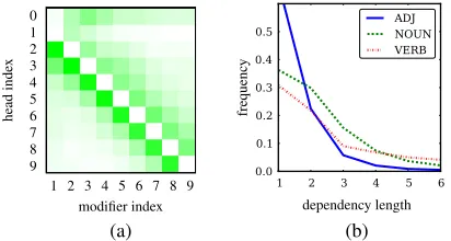
Figure 1: (a) Heat map indicating how likely a par-ticular head position is for each modifier position. Greener/darker is likelier. (b) Arc length frequency for three common modifier tags. Both charts are computed from all sentences in Section 22 of the PTB.

(2002) shows is a practical lower bound for parsing of context-free grammars. This bound implies that it is unlikely that there can be an exhaustive pars-ing algorithm that is asymptotically faster than the standard approach.

We thus need to leverage domain knowledge to obtain faster parsing algorithms. It is well-known that natural language is fairly linear, and most head-modifier dependencies tend to be short. This prop-erty is exploited by transition-based dependency parsers (Yamada and Matsumoto, 2003; Nivre et al., 2004) and empirically demonstrated in Figure 1. The heat map on the left shows that most of the probability mass of modifiers is concentrated among nearby words, corresponding to a diagonal band in the matrix representation. On the right we show the frequency of arc lengths for different modifier part-of-speech tags. As one can expect, almost all arcs involving adjectives (ADJ) are very short (length3

or less), but even arcs involving verbs and nouns are often short. This structure suggests that it may be possible to disambiguate most dependencies by con-sidering only the “banded” portion of the sentence.

We exploit this linear structure by employing a variant of vine parsing (Eisner and Smith, 2005).2 Vine parsing is a dependency parsing algorithm that considers only close words as modifiers. Because of this assumption it runs in linear time. Of course, any parse tree with hard limits on dependency lengths will contain major parse errors. We therefore use the

2_{The term vine parsing is a slight misnomer, since the}

As McGwire neared , fans went wild

* * As McGwire neared , fans went wild * As McGwire neared , fans went wild

modifiers

heads

As McGwire neared , _{fans went wild} *

As McGwire neared , fans went wild

modifiers

heads

As McGwire neared , _{fans went wild} *

As McGwire neared , fans went wild

modifiers

heads

As McGwire neared , _{fans went wild} *

As McGwire neared , fans went wild

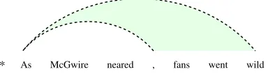
Figure 2: Multi-pass pruning with a vine, first-order, and second-order model shown as dependencies and filtered index sets after each pass. Darker cells have higher max-marginal values, while empty cells represent pruned arcs.

vine parser only for pruning and augment it to allow arcs to remain unspecified (by including so called

outer arcs). The vine parser can thereby eliminate

a possibly quadratic number of arcs, while having the flexibility to defer some decisions and preserve ambiguity to be resolved by later passes. In Figure 2 for example, the vine pass correctly determined the head-word ofMcGwireasneared, limited the

head-word candidates for fans to neared and went, and

decided that the head-word forwentfalls outside the

band by proposing an outer arc. A subsequent first-order pass needs to score only a small fraction of all possible arcs and can be used to further restrict the search space for the following higher-order passes.

3 Graph-Based Dependency Parsing

Graph-based dependency parsing models factor all valid parse trees for a given sentence into smaller units, which can be scored independently. For in-stance, in a first-order factorization, the units are just dependency arcs. We represent these units by an in-dex set I and use binary vectors Y ⊂ {0,1_}|I| to

specify a parse treey∈ Ysuch thaty(i) = 1iff the

indexiexists in the tree. The index sets of

higher-order models can be constructed out of the index sets of lower-order models, thus forming a hierarchy that we will exploit in our coarse-to-fine cascade.

The inference problem is to find the 1-best parse treearg maxy_∈Yy·w, wherew ∈R|I|is a weight

vector that assigns a score to each indexi(we

dis-cuss how w is learned in Section 4). A

general-ization of the 1-best inference problem is to find the max-marginal score for each index i.

Max-marginals are given by the functionM :_{I → Y}

de-fined asM(i;_Y, w) = arg max_y∈Y:y(i)=1y_·w. For

first-order parsing, this corresponds to the best parse utilizing a given dependency arc. Clearly there are exponentially many possible parse tree structures, but fortunately there exist well-known dynamic pro-gramming algorithms for searching over all possible structures. We review these below, starting with the first-order factorization for ease of exposition.

Throughout the paper we make use of some ba-sic mathematical notation. We write[c]for the

enu-meration{1, . . . , c}and[c]afor{a, . . . , c}. We use 1[c] for the indicator function, equal to 1 if

con-dition c is true and 0 otherwise. Finally we use [c]+= max{0, c}for the positive part ofc.

3.1 First-Order Parsing

The simplest way to index a dependency parse struc-ture is by the individual arcs of the parse tree. This model is known as first-order or arc-factored. For a sentence of lengthnthe index set is:

I1 ={(h, m) :h∈[n]0, m∈[n]}

Each dependency tree hasy(h, m) = 1iff it includes

an arc from headhto modifierm. We follow

com-mon practice and use position0as the pseudo-root

(∗) of the sentence. The full set I1 has cardinality

(a)

h m

← I

h r

+ C

m r+ 1

C

(b)

h e

← C

h m

+ I

m e

C

Figure 3: Parsing rules for first-order dependency

pars-ing. The complete itemsCare represented by triangles

and the incomplete itemsIare represented by trapezoids.

Symmetric left-facing versions are also included.

The first-order bilexical parsing algorithm of Eis-ner (2000) can be used to find the best parse tree and max-marginals. The algorithm defines a dy-namic program over two types of items:

incom-plete items I(h, m) that denote the span between

a modifier m and its head h, and complete items C(h, e)that contain a full subtree spanning from the

head h and to the word e on one side. The

algo-rithm builds larger items by applying the composi-tion rules shown in Figure 3. Rule 3(a) builds an incomplete itemI(h, m)by attachingmas a

modi-fier toh. This rule has the effect thaty(h, m) = 1in

the final parse. Rule 3(b) completes itemI(h, m)by

attaching item C(m, e). The existence of I(h, m)

implies thatmmodifiesh, so this rule enforces that

the constituents ofmare also constituents ofh.

We can find the best derivation for each item by adapting the standard CKY parsing algorithm to these rules. Since both rule types contain three variables that can range over the entire sentence (h, m, e∈[n]0), the bottom-up, inside dynamic

pro-gramming algorithm requiresO(n3)time.

Further-more, we can find max-marginals with an additional top-down outside pass also requiring cubic time. To speed up search, we need to filter indices from I1

and reduce possible applications of Rule 3(a).

3.2 Higher-Order Parsing

Higher-order models generalize the index set by us-ing siblus-ingss(modifiers that previously attached to

a head word) and grandparentsg(head words above

the current head word). For compactness, we useg1

for the head word andsk+1for the modifier and

pa-rameterize the index set to capture arbitrary

higher-(c) V←

0 e

←C

0 e−1 +

e e−1 C

(d)

0 e

←

V←

0 m

+ V←

e m I

(e)

0 e

←

V→

0 e

V←

(f)

0 e

←

V→

0 m

+ V→

e m I

(g)

0 e

←

C

0 e−1 + V→

e−1 e C

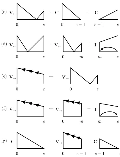
Figure 4: Additional rules for vine parsing. Vine left (V←) items are pictured as right-facing triangles and vine

right (V→) items are marked trapezoids. Each new item

is anchored at the root and grows to the right.

order decisions in both directions:

Ik,l ={(g, s) :g∈[n]l0+1, s∈[n] k+1

}

where k+ 1 is the sibling order, l+ 1 is the

par-ent order, and k +l+ 1 is the model order. The

canonical second-order model usesI1,0, which has

a cardinality ofO(n3). Although there are several

possibilities for higher-order models, we useI1,1as

our third-order model. Generally, the parsing index set has cardinality |Ik,l| = O(n2+k+l). Inference

in higher-order models uses variants of the dynamic program for first-order parsing, and we refer to pre-vious work for the full set of rules. For second-order models with index setI1,0, parsing can be done in O(n3) time (McDonald and Pereira, 2006) and for

third-order models inO(n4)time (Koo and Collins,

2010). Even though second-order parsing has the same asymptotic time complexity as first-order pars-ing, inference is significantly slower due to the cost of scoring the larger index set.

that can be pruned using a coarse pruning model. For example, to use a first-order model for pruning, we would map the higher-order index to the individ-ual indices for its arc, grandparents, and siblings:

pk,l→1(g, s) = {(g1, sj) :j∈[k+ 1]} ∪ {(gj+1, gj) :j∈[l]}

The first-order pruning model can then be used to score these indices, and to produce a filtered in-dex setF(I1)by removing low-scoring indices (see

Section 4). We retain only the higher-order indices that are supported by the filtered index set:

{(g, s)∈ Ik,l :pk,l→1(g, s)⊂F(I1)}

3.3 Vine Parsing

To further reduce the cost of parsing and produce faster pruning models, we need a model with less structure than the first-order model. A natural choice, following Section 2, is to only consider “short” arcs:

S ={(h, m)∈ I1 : |h−m| ≤b}

wherebis a small constant. This constraint reduces

the size of the set to|S|=O(nb).

Clearly, this index set is severely limited; it is nec-essary to have some long arcs for even short sen-tences. We therefore augment the index set to in-cludeouterarcs:

I0 =S ∪ {(d, m) :d∈ {←,→}, m∈[n]} ∪ {(h, d) :h∈[n]0, d∈ {←,→}}

The first set lets modifiers choose an outer head-word and the second set lets head head-words accept outer modifiers, and both sets distinguish the direction of the arc. Figure 5 shows a right outer arc. The size of

I0 is linear in the sentence length. To parse the

in-dex setI0, we can modify the parse rules in Figure 3 to enforce additional length constraints (|h₋e_{| ≤}b

forI(h, e)and_|h₋m_{| ≤}bforC(h, m)). This way,

only indices inSare explored. Unfortunately, this is not sufficient since the constraints also prevent the algorithm from producing a full derivation, since no item can expand beyond lengthb.

Eisner and Smith (2005) therefore introduce vine parsing, which includes two new items, vine left,

As McGwire neared , fans went wild *

Figure 5: An outer arc(1,_→)from the word “As” to

pos-sible right modifiers.

V_←(e), andvine right,V_→(e). Unlike the previous

items, these new items are left-anchored at the root and grow only towards the right. The itemsV_←(e)

and V_→(e) encode the fact that a word e has not

taken a close (withinb) head word to its left or right.

We incorporate these items by adding the five new parsing rules shown in Figure 4.

The major addition is Rule 4(e) which converts a vine left itemV_←(e)to a vine right itemV_→(e). This

implies that wordehas no close head to either side,

and the parse has outer head arcs,y(←, e) = 1 or y(_→, e) = 1. The other rules are structural and

dic-tate creation and extension of vine items. Rules 4(c) and 4(d) create vine left items from items that can-not find a head word to their left. Rules 4(f) and 4(g) extend and finish vine right items. Rules 4(d) and 4(f) each leave a head word incomplete, so they may set y(e,_←) = 1 or y(m,_→) = 1

respec-tively. Note that for all the new parse rules,e_∈[n]0

andm _{∈ {}e₋b . . . n_}, so parsing time of this so

called vine parsing algorithm is linear in the sen-tence lengthO(nb2).

Alone, vine parsing is a poor model of syntax - it does not even score most dependency pairs. How-ever, it can act as a pruning model for other parsers. We prune a first-order model by mapping first-order indices to indices inI0.

p1→0(h, m) =







{(h, m)_} if_|h₋m_{| ≤}b {(_→, m),(h,_→)_} ifh < m {(←, m),(h,←)} ifh > m

The remaining first-order indices are then given by:

{(h, m)_{∈ I1} :p1→0(h, m)⊂F(I0)}

4 Training Methods

Our coarse-to-fine parsing architecture consists of multiple pruning passes followed by a final pass of 1-best parsing. The training objective for the pruning models comes from the prediction cascade framework of Weiss and Taskar (2010), which ex-plicitly trades off pruning efficiency versus accuracy. The models used in the final pass on the other hand are trained for 1-best prediction.

4.1 Max-Marginal Filtering

At each pass of coarse-to-fine pruning, we apply an index filter functionF to trim the index set:

F(_I) =_{i_{∈ I} :f(i) = 1_}

Several types of filters have been proposed in the literature, with most work in coarse-to-fine pars-ing focuspars-ing on predicates that threshold the poste-rior probabilities. In structured prediction cascades, we use a non-probabilistic filter, based on the max-marginal value of the index:

f(i;_Y, w) =1[M(i;_Y, w)_·w < tα(_Y, w) ]

where tα(Y, w) is a sentence-specific threshold

value. To counteract the fact that the max-marginals are not normalized, the thresholdtα(_Y, w)is set as

a convex combination of the 1-best parse score and the average max-marginal value:

tα(Y, w) = αmax y∈Y (y·w)

+ (1₋α) 1 |I|

X

i∈I

M(i;_Y, w)_·w

where the model-specific parameter0 ≤ α ≤ 1is

the tradeoff betweenα= 1, pruning all indicesinot

in the best parse, andα= 0, pruning all indices with

max-marginal value below the mean.

The threshold function has the important property that for any parsey, ify_·w_≥tα(Y, w)theny(i) = 1implies f(i) = 0, i.e. if the parse score is above

the threshold, then none of its indices will be pruned.

4.2 Filter Loss Training

The aim of our pruning models is to filter as many indices as possible without losing the gold parse. In

structured prediction cascades, we incorporate this pruning goal into our training objective.

Letybe the gold output for a sentence. We define

filter loss to be an indicator of whether any iwith

y(i) = 1is filtered:

∆(y,_Y, w) =1[_∃i_∈y, M(i;_Y, w)_·w < tα(Y, w)]

During training we minimize the expected filter loss using a standard structured SVM setup (Tsochan-taridis et al., 2006). First we form a convex, con-tinuous upper-bound of our loss function:

∆(y,Y, w) ≤ 1[y·w < tα(Y, w)] ≤ [1−y·w+tα(Y, w)]+

where the first inequality comes from the proper-ties of max-marginals and the second is the standard hinge-loss upper-bound on an indicator.

Now assume that we have a corpus of P

train-ing sentences. Let the sequence(y(1), . . . , y(P)) be

the gold parses for each sentences and the sequence

(Y(1)_{, . . . ,Y}(P)_{)be the set of possible output}

struc-tures. We can form the regularized risk minimiza-tion for this upper bound of filter loss:

min w λkwk

2₊ 1 P

P

X

p=1

[1−y(p)·w+tα(Y(p)_{, w)]} +

This objective is convex and non-differentiable, due to the max insidet. We optimize using stochastic

subgradient descent (Shalev-Shwartz et al., 2007). The stochastic subgradient at examplep,H(w, p)is 0ify(p)₋1_≥tα(Y, w)otherwise,

H(w, p) = 2λw P −y

(p)_{+αarg max}

y∈Y(p)y·w + (1−α) 1

|I(p)_|

X

i∈I(p)

M(i;Y(p)_{, w)}

Each step of the algorithm has an update of the form:

wk=wk−1−ηkH(w, p)

whereη is an appropriate update rate for

subgradi-ent convergence. Ifα = 1the objective is identical

to structured SVM with 0/1 hinge loss. For other values of α, the subgradient includes a term from

First-order Second-order Third-order

Setup Speed PE Oracle UAS Speed PE Oracle UAS Speed PE Oracle UAS

NOPRUNE 1.00 0.00 100 91.4 0.32 0.00 100 92.7 0.01 0.00 100 93.3

LENGTHDICTIONARY 1.94 43.9 99.9 91.5 0.76 43.9 99.9 92.8 0.05 43.9 99.9 93.3

LOCALSHORT 3.08 76.6 99.1 91.4 1.71 76.4 99.1 92.6 0.31 77.5 99.0 93.1

LOCAL 4.59 89.9 98.8 91.5 2.88 83.2 99.5 92.6 1.41 89.5 98.8 93.1

FIRSTONLY 3.10 95.5 95.9 91.5 2.83 92.5 98.4 92.6 1.61 92.2 98.5 93.1

FIRSTANDSECOND - - 1.80 97.6 97.7 93.1

VINEPOSTERIOR 3.92 94.6 96.5 91.5 3.66 93.2 97.7 92.6 1.67 96.5 97.9 93.1

VINECASCADE 5.24 95.0 95.7 91.5 3.99 91.8 98.7 92.6 2.22 97.8 97.4 93.1

k=8 k=16 k=64

ZHANGNIVRE 4.32 - - 92.4 2.39 - - 92.5 0.64 - - 92.7

Table 1: Results comparing pruning methods on PTB Section 22. Oracle is the max achievable UAS after pruning. Pruning efficiency (PE) is the percentage of non-gold first-order dependency arcs pruned. Speed is parsing time relative to the unpruned first-order model (around 2000 tokens/sec). UAS is the unlabeled attachment score of the final parses.

4.3 1-Best Training

For the final pass, we want to train the model for 1-best output. Several different learning methods are available for structured prediction models including structured perceptron (Collins, 2002), max-margin models (Taskar et al., 2003), and log-linear mod-els (Lafferty et al., 2001). In this work, we use the margin infused relaxed algorithm (MIRA) (Cram-mer and Singer, 2003; Cram(Cram-mer et al., 2006) with a hamming-loss margin. MIRA is an online algo-rithm with similar benefits as structured perceptron in terms of simplicity and fast training time. In prac-tice, we found that MIRA with hamming-loss mar-gin gives a performance improvement over struc-tured perceptron and strucstruc-tured SVM.

5 Parsing Experiments

To empirically demonstrate the effectiveness of our approach, we compare our vine pruning cascade with a wide range of common pruning methods on the Penn WSJ Treebank (PTB) (Marcus et al., 1993). We then also show that vine pruning is effective across a variety of different languages.

For English, we convert the PTB constituency trees to dependencies using the Stanford dependency framework (De Marneffe et al., 2006). We then train on the standard PTB split with sections 2-21 as training, section 22 as validation, and section 23 as test. Results are similar using the Yamada and Matsumoto (2003) conversion. We additionally se-lected six languages from the CoNLL-X shared task

(Buchholz and Marsi, 2006) that cover a number of different language families: Bulgarian, Chinese, Japanese, German, Portuguese, and Swedish. We use the standard CoNLL-X training/test split and tune parameters with cross-validation.

All experiments use unlabeled dependencies for training and test. Accuracy is reported as unlabeled attachment score (UAS), the percentage of tokens with the correct head word. For English, UAS ig-nores punctuation tokens and the test set uses pre-dicted POS tags. For the other languages we fol-low the CoNLL-X setup and include punctuation in UAS and use gold POS tags on the set set. Speed-ups are given in terms of time relative to a highly optimized C++ implementation. Our unpruned first-order baseline can process roughly two thousand to-kens a second and is comparable in speed to the greedy shift-reduce parser of Nivre et al. (2004).

5.1 Models

Our parsers perform multiple passes over each sen-tence. In each pass we first construct a (pruned) hy-pergraph (Klein and Manning, 2005) and then per-form feature computation and inference. We choose the highest α that produces a pruning error of no

more than 0.2 on the validation set (typicallyα ≈ 0.6) to filter indices for subsequent rounds (similar

to Weiss and Taskar (2010)). We compare a variety of pruning models:

LENGTHDICTIONARY a deterministic

head-modifier POS pair.

LOCAL an unstructured arc classifier that chooses

indices from I1 directly without enforcing parse constraints. Similar to the quadratic-time filter from Bergsma and Cherry (2010). LOCALSHORT an unstructured arc classifier that

chooses indices from I0 directly without

en-forcing parse constraints. Similar to the linear-time filter from Bergsma and Cherry (2010). FIRSTONLY a structured first-order model trained

with filter loss for pruning.

FIRSTANDSECOND a structured cascade with

first- and second-order pruning models. VINECASCADE the full cascade with vine,

first-and second-order pruning models.

VINEPOSTERIOR the vine parsing cascade trained

as a CRF with L-BFGS (Nocedal and Wright, 1999) and using posterior probabilities for fil-tering instead of max-marginals.

ZHANGNIVRE an unlabeled reimplementation of

the linear-time, k-best, transition-based parser of Zhang and Nivre (2011). This parser uses composite features up to third-order with a greedy decoding algorithm. The reimplemen-tation is about twice as fast as their reported speed, but scores slightly lower.

We found LENGTHDICTIONARY pruning to give

significant speed-ups in all settings and therefore al-ways use it as an initial pass. The maximum number of passes in a cascade is five: dictionary, vine, first-, and second-order pruning, and a final third-order 1-best pass.3 _{We tune the pruning thresholds for each} round and each cascade separately. This is because we might be willing to do a more aggressive vine pruning pass if the final model is a first-order model, since these two models tend to often agree.

5.2 Features

For the non-pruning models, we use a standard set of features proposed in the discriminative graph-based dependency parsing literature (McDonald et al., 2005; Carreras, 2007; Koo and Collins, 2010).

3_{For the first-order parser, we found it beneficial to employ a}

reduced feature first-order pruner before the final model, i.e. the cascade has four rounds: dictionary, vine, first-order pruning, and first-order 1-best.

sentence length

10 20 30 40 50 No Prune [2.8] Length [1.9] Cascade [1.4]

mean

time

first-order

sentence length

10 20 30 40 50 No Prune [2.8] Length [2.0] Cascade [1.8]

mean

time

second-order

sentence length

10 20 30 40 50 No Prune [3.8] Length [2.4] Cascade [1.9]

mean

time

third-order

sentence length

10 20 30 40 50 Length [1.9]

Local [1.8] Cascade [1.4]

mean

time

pruning methods

Figure 6: Mean parsing speed by sentence length for first-, second-, and third-order parsers as well as

differ-ent pruning methods for first-order parsing. [b]indicates

the empirical complexity obtained from fittingaxb_.

Included are lexical features, part-of-speech tures, features on in-between tokens, as well as fea-ture conjunctions, surrounding part-of-speech tags, and back-off features. In addition, we replicate each part-of-speech (POS) feature with an additional fea-ture using coarse POS representations (Petrov et al., 2012). Our baseline parsing models replicate and, for some experiments, surpass previous best results. The first- and second-order pruning models have the same structure, but for efficiency use only the basic features from McDonald et al. (2005). As fea-ture computation is quite costly, fufea-ture work may investigate whether this set can be reduced further. VINEPRUNEand LOCALSHORT use the same

fea-ture sets for short arcs. Outer arcs have feafea-tures of the unary head or modifier token, as well as features for the POS tag bordering the cutoff and the direc-tion of the arc.

5.3 Results

A comparison between the pruning methods is shown in Table 1. The table gives relative speed-ups, compared to the unpruned first-order baseline, as well as accuracy, pruning efficiency, and ora-cle scores. Note particularly that the third-order cascade is twice as fast as an unpruned first-order model and >200 times faster than the unpruned

poste-1-Best Model

Round First Second Third

Vine 37% 27% 16%

First 63% 30% 17%

Second - 43% 18%

Third - - 49%

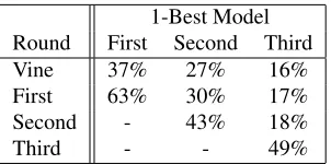
Table 2: Relative speed of pruning models in a multi-pass cascade. Note that the 1-best models use richer features than the corresponding pruning models.

rior pruning is less pronounced. Filter loss train-ing is faster than VINEPOSTERIOR for first- and

third-order parsing, but the two models have similar second-order speeds. It is also noteworthy that ora-cle scores are consistently high even after multiple pruning rounds: the oracle score of our third-order model for example is 97.4%.

Vine pruning is particularly effective. The vine pass is faster than both LOCAL and FIRSTONLY

and prunes more effectively than LOCALSHORT.

Vine pruning benefits from having a fast, linear-time model, but still maintaining enough structure for pruning. While our pruning approach does not pro-vide any asymptotic guarantees, Figure 6 shows that in practice our multi-pass parser scales well even for long sentences: Our first-order cascade scales almost linearly with the sentence length, while the third-order cascade scales better than quadratic. Ta-ble 2 shows that the final pass dominates the compu-tational cost, while each of the pruning passes takes up roughly the same amount of time.

Our second- and third-order cascades also signif-icantly outperform ZHANGNIVRE. The

transition-based model withk = 8is very efficient and

effec-tive, but increasing thek-best list size scales much

worse than employing multi-pass pruning. We also note that while direct speed comparison are difficult, our parser is significantly faster than the published results for other high accuracy parsers, e.g. Huang and Sagae (2010) and Koo et al. (2010).

Table 3 shows our results across a subset of the CoNLL-X datasets, focusing on languages that dif-fer greatly in structure. The unpruned models per-form well across datasets, scoring comparably to the top results from the CoNLL-X competition. We see speed increases for our cascades with almost no loss in accuracy across all languages, even for languages with fairly free word order like German. This is

First-order Second-order Third-order

Setup Speed UAS Speed UAS Speed UAS

BG B 1.90 90.7 0.67 92.0 0.05 92.1

V 6.17 90.5 5.30 91.6 1.99 91.9

DE B 1.40 89.2 0.48 90.3 0.02 90.8

V 4.72 89.0 3.54 90.1 1.44 90.8

JA B 1.77 92.0 0.58 92.1 0.04 92.4

V 8.14 91.7 8.64 92.0 4.30 92.3

PT B 0.89 90.1 0.28 91.2 0.01 91.7

V 3.98 90.0 3.45 90.9 1.45 91.5

SW B 1.37 88.5 0.45 89.7 0.01 90.4

V 6.35 88.3 6.25 89.4 2.66 90.1

ZH B 7.32 89.5 3.30 90.5 0.67 90.8

V 7.45 89.3 6.71 90.3 3.90 90.9

EN B 1.0 91.2 0.33 92.4 0.01 93.0

V 5.24 91.0 3.92 92.2 2.23 92.7

Table 3: Speed and accuracy results for the vine pring cascade across various languages. B is the un-pruned baseline model, and V is the vine pruning cas-cade. The first section of the table gives results for

the CoNLL-X test datasets for Bulgarian (BG), German

(DE), Japanese (JA), Portuguese (PT), Swedish (SW),

and Chinese (ZH). The second section gives the result

for the English (EN) test set, PTB Section 23.

encouraging and suggests that the outer arcs of the vine-pruning model are able to cope with languages that are not as linear as English.

6 Conclusion

We presented a multi-pass architecture for depen-dency parsing that leverages vine parsing and struc-tured prediction cascades. The resulting 200-fold speed-up leads to a third-order model that is twice as fast as an unpruned first-order model for a vari-ety of languages, and that also compares favorably to a state-of-the-art transition-based parser. Possible future work includes experiments using cascades to explore much higher-order models.

Acknowledgments

References

S. Bergsma and C. Cherry. 2010. Fast and accurate arc

filtering for dependency parsing. InProc. of COLING,

pages 53–61.

S. Buchholz and E. Marsi. 2006. CoNLL-X shared task

on multilingual dependency parsing. InCoNLL.

X. Carreras, M. Collins, and T. Koo. 2008. Tag, dynamic programming, and the perceptron for efficient,

feature-rich parsing. InProc. of CoNLL, pages 9–16.

X. Carreras. 2007. Experiments with a higher-order

projective dependency parser. In Proc. of CoNLL

Shared Task Session of EMNLP-CoNLL, volume 7, pages 957–961.

E. Charniak, M. Johnson, M. Elsner, J. Austerweil, D. Ellis, I. Haxton, C. Hill, R. Shrivaths, J. Moore, M. Pozar, et al. 2006. Multilevel coarse-to-fine PCFG

parsing. InProc. of NAACL/HLT, pages 168–175.

M. Collins. 2002. Discriminative training methods for hidden markov models: Theory and experiments with

perceptron algorithms. InProc. of EMNLP, pages 1–8.

K. Crammer and Y. Singer. 2003. Ultraconservative

on-line algorithms for multiclass problems. The Journal

of Machine Learning Research, 3:951–991.

K. Crammer, O. Dekel, J. Keshet, S. Shalev-Shwartz, and Y. Singer. 2006. Online passive-aggressive

algo-rithms. The Journal of Machine Learning Research,

7:551–585.

M.C. De Marneffe, B. MacCartney, and C.D. Manning.

2006. Generating typed dependency parses from

phrase structure parses. InProc. of LREC, volume 6,

pages 449–454.

J. Eisner and N.A. Smith. 2005. Parsing with soft and

hard constraints on dependency length. In Proc. of

IWPT, pages 30–41.

J. Eisner. 2000. Bilexical grammars and their

cubic-time parsing algorithms. Advances in Probabilistic

and Other Parsing Technologies, pages 29–62. L. Huang and K. Sagae. 2010. Dynamic programming

for linear-time incremental parsing. InProc. of ACL,

pages 1077–1086.

D. Klein and C.D. Manning. 2005. Parsing and

hy-pergraphs. New developments in parsing technology,

pages 351–372.

T. Koo and M. Collins. 2010. Efficient third-order

de-pendency parsers. InProc. of ACL, pages 1–11.

T. Koo, A.M. Rush, M. Collins, T. Jaakkola, and D. Son-tag. 2010. Dual decomposition for parsing with

non-projective head automata. InProc. of EMNLP, pages

1288–1298.

M. Kuhlmann, C. G´omez-Rodr´ıguez, and G. Satta. 2011. Dynamic programming algorithms for

transition-based dependency parsers. In Proc. of ACL/HLT,

pages 673–682.

J. Lafferty, A. McCallum, and F.C.N. Pereira. 2001. Conditional random fields: Probabilistic models for

segmenting and labeling sequence data. In Proc. of

ICML, pages 282–289.

L. Lee. 2002. Fast context-free grammar parsing

re-quires fast boolean matrix multiplication. Journal of

the ACM, 49(1):1–15.

M.P. Marcus, M.A. Marcinkiewicz, and B. Santorini.

1993. Building a large annotated corpus of

en-glish: The penn treebank. Computational linguistics,

19(2):313–330.

R. McDonald and F. Pereira. 2006. Online learning of

approximate dependency parsing algorithms. InProc.

of EACL, volume 6, pages 81–88.

R. McDonald, K. Crammer, and F. Pereira. 2005. Online

large-margin training of dependency parsers. InProc.

of ACL, pages 91–98.

J. Nivre, J. Hall, and J. Nilsson. 2004. Memory-based

dependency parsing. InProc. of CoNLL, pages 49–56.

J. Nocedal and S. J. Wright. 1999.Numerical

Optimiza-tion. Springer.

A. Pauls and D. Klein. 2009. Hierarchical search for

parsing. InProc. of NAACL/HLT, pages 557–565.

S. Petrov and D. Klein. 2007. Improved inference for

unlexicalized parsing. InProc. of NAACL/HLT, pages

404–411.

S. Petrov, D. Das, and R. McDonald. 2012. A universal

part-of-speech tagset. InLREC.

S. Petrov. 2009. Coarse-to-Fine Natural Language

Processing. Ph.D. thesis, University of California at Bekeley, Berkeley, CA, USA.

B. Roark and K. Hollingshead. 2008. Classifying chart cells for quadratic complexity context-free inference. InProc. of COLING, pages 745–751.

S. Shalev-Shwartz, Y. Singer, and N. Srebro. 2007. Pe-gasos: Primal estimated sub-gradient solver for svm. InProc. of ICML, pages 807–814.

B. Taskar, C. Guestrin, and D. Koller. 2003. Max-margin

markov networks. Advances in neural information

processing systems, 16:25–32.

I. Tsochantaridis, T. Joachims, T. Hofmann, and Y. Al-tun. 2006. Large margin methods for structured and

interdependent output variables. Journal of Machine

Learning Research, 6(2):1453.

D. Weiss and B. Taskar. 2010. Structured prediction

cas-cades. InProc. of AISTATS, volume 1284, pages 916–

923.

H. Yamada and Y. Matsumoto. 2003. Statistical

depen-dency analysis with support vector machines. InProc.

of IWPT, volume 3, pages 195–206.

Y. Zhang and J. Nivre. 2011. Transition-based

depen-dency parsing with rich non-local features. InProc. of