Optimized Feedback Control of Vortex Shedding on an Inclined Flat Plate

Inclined Flat Plate

Thesis by

Won Tae Joe

In Partial Fulfillment of the Requirements for the Degree of

Doctor of Philosophy

California Institute of Technology Pasadena, California

2010

To my parents, JangHo and JaKyung Joe, and

Acknowledgments

My advisor, Professor Tim Colonius, is gratefully acknowledged for his support and teachings throughout my graduate studies. His passion for research and science has been a great inspira-tion. I thank him for all his patience in guiding me through the road to become a better scientist and and also for the countless revisions to my papers. It has been a true joy and an unparalleled learning experience. I would also like to acknowledge Doctor Douglas MacMynowski for his guidance and critical comments on controls and dynamics in order to make the design and implementation of the feedback system possible. Professors Fazle Hussain, Morteza Gharib, and Beverly McKeon have offered enlightening comments and graciously agreed to serve on my committee.

I was also fortunate to have been involved in a multi-disciplinary research initiative (MURI), receiving insightful comments by Professors Clarence Rowley (Princeton Univ), David Williams (Illinois Inst of Tech), Gilead Tadmor (Northeastern Univ), and Doctor William Dickson. Funding for this research was provided by the U.S. Air Force Office of Scientific Research and some of the computations were made possible by the U.S. Department of Defense High Performance Computing Modernization Program. I must also thank Professor Colm Caulfield (University of California, San Diego, now at University of Cambridge) for his guidance during my undergraduate studies. He has been a great motivation for me both, in my rst scientic research project, and in my continued pursuit of graduate-level studies.

have helped immensely in creating a life outside of the lab, which has given me mental and emotional stability throughout my Caltech tenure.

Additionally, I would like to thank my previous roommates from University of California, San Diego, Andy Yoon and Larry Chae, for helping shape my character during our college days and for providing continual emotional and mental support.

Abstract

This thesis examines flow control and the potentially favorable effects of feedback, associated with unsteady actuation in separated flows over airfoils. The objective of the flow control is to enhance lift at post-stall angles of attack by changing the dynamics of the wake vortices. We present results from a numerical study of unsteady actuation on a two-dimensional flat plate at post-stall angles of attack at Reynolds number (Re) of 300 and 3000. At Re = 300, the control waveform is optimized and a feedback strategy is developed to optimize the phase of the control relative to the lift with either a sinusoidal or the optimized waveform, resulting in a high-lift limit cycle of vortex shedding. Also at Re = 3000, we show that certain frequencies and actuator waveforms lead to stable (high-lift) limit cycles, in which the flow is phase locked to the actuation

First, a two-dimensional flat plate model at a high angle of attack at a Re of 300 is considered. With the sinusoidal forcing, we find that certain phase shifts between the forcing and lift signals result in very high period-averaged lifts. We design the feedback to slightly adjust the frequency and/or phase of actuation to lock it to a particular phase of the lift, thus achieving a phase-locked flow with the maximal period-averaged lift over every cycle of acutation.

Optimal control provides a periodic control waveform, resulting in high lift shedding cycle with minimal control input. However, if applied in open loop, the flow fails to phase lock onto the optimal waveform, degrading the lift performance. Thus, the optimized waveform is also implemented in a closed-loop controller where the control signal is shifted or deformed periodically to adjust to the (instantaneous) frequency of the lift fluctuations. The feedback utilizes a narrowband filter and an Extended Kalman Filter to robustly estimate the phase of vortex shedding and achieve phase-locked, high lift flow states. Feedback control of the optimized waveform is able to reproduce the high-lift limit cycle from the optimization, but starting from an arbitrary phase of the baseline limit cycle.

Contents

Acknowledgments iv

Abstract vi

Contents viii

List of Figures xi

Nomenclature xvi

1 Introduction 1

1.1 Background of Flow Control. . . 3

1.2 Open-Loop Control. . . 5

1.3 Feedback Control . . . 6

1.4 Overview of Current Work. . . 7

2 Numerical Methods 10 2.1 Fast Immersed Boundary Method. . . 10

3 Sinusoidal Forcing at Re= 300 16 3.1 Numerical Method . . . 16

3.2 Results. . . 18

3.2.1 Uncontrolled Flow . . . 18

3.2.2.1 Leading-edge actuation . . . 19

3.2.2.2 Trailing-edge actuation . . . 24

3.3 Closed-loop control . . . 26

4 Optimized waveform at Re= 300 37 4.1 Numerical Method . . . 38

4.2 Adjoint-based Optimization . . . 39

4.2.1 Adjoint-based Optimization: Cost Functional and Sensitivity . . . 39

4.2.2 Adjoint-based Optimization: Formulation . . . 40

4.2.3 Adjoint-based Optimization: Numerical Implementation . . . 42

4.2.4 Adjoint-based Optimization: Results . . . 44

4.3 Feedback . . . 45

4.4 Results of Optimized Feedback Control . . . 47

4.5 Sinusoidal Pulse . . . 52

5 Control at Re= 3000 56 5.1 Numerical Method . . . 57

5.2 Uncontrolled flow . . . 61

5.3 Actuation atα= 10◦_{. . . . 62}

5.4 Actuation atα= 20◦_{. . . . 69}

6 Conclusions 83 6.1 Control at Re = 300 . . . 84

6.1.1 Sinusoidal Forcing . . . 84

6.1.2 Optimization of the Control Waveform. . . 85

6.1.3 Feedback Control with the Optimized Waveform . . . 86

6.2 Control atRe= 3000 . . . 87

Appendix A Appendix A 91

A.1 Derivation of Linearized and Adjoint Equations . . . 91

Appendix B Appendix B 94

B.1 Extended Kalman Filter . . . 94

List of Figures

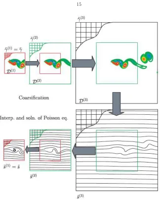
2.1 Multi-domain method to solve the Poisson equation. Figure reproduced with

permis-sion from Colonius & Taira (2008). . . 15

3.1 Schematic of actuation at leading and trailing edge. . . 18

3.2 Vorticity and streamlines of translating flat plate at different angle of attack, α at

Re= 300. . . 20

3.3 Leading-edge actuation: maximum and minimum lift () and its average over time (

◦

for downstream (left) and upstream (right) actuation. Average of the baseline case is

plotted in dashed grey and shaded region is bounded by its maximum and minimum.

Actuation is applied at the natural shedding frequency,ωf =ωn. For cases where the

flow is not phase locked to the forcing signal, variation in period-averaged lift over

each actuation period is plotted with error bar to indicate the range of values over a

subharmonic limit cycle.. . . 22

3.4 Lift as a function of time (a) and jet velocity (b) with upstream actuation at the leading

edge (LE, upstream) at the natural shedding frequency (ωf =ωn) forα= 50◦_{. . . . . 23} 3.5 Trailing-edge actuation: see Figure 3.3 for a description.. . . 27

3.6 Lift with upstream actuation at the trailing-edge at it natural shedding frequency

(ωf=ωn), forα= 50◦_{. . . . . 28} 3.7 Vorticity contour at the time of maximum lift for baseline (thin) and upstream

actua-tion (thick) at the trailing edge at the natural shedding frequency (ωf =ωn). Dashed

3.8 Vorticity contour at the time of maximum lift for baseline (black) and upstream

actu-ation (red) at the trailing edge at the natural shedding frequency (ωf =ωn). . . 29

3.9 Trailing-edge actuation: maximum and minimum lift (), average lift (

◦

period-averaged lift (error bar) over a range of open-loop forcing frequency,ωf. Maximum and

minimum lift of baseline (- - -) case is shown as a reference. . . 30

3.10 Trailing-edge actuation: phase shift of the forcing signal,Uj, relative to the lift signal,

CL, for phase-locked flows, over a range of open-loop forcing frequency,ωf (α= 30◦_{). 31} 3.11 Feedback control configuration. . . 31

3.12 Maximum and minimum lift () and its average over time (

◦

(bottom) of phase-locked limit cycles at different phase-shift,φo, for (a)α= 40◦ _and

(b) 50◦. . . 35

3.13 Comparison between open-loop control case (–), that phase locked the flow at the

highest averageCL(denoted as OL1in Figure 3.9(c)), and the corresponding feedback

control case (–) (denoted as FB1 in Figure 3.12). Forcing frequency of this open-loop

control is denoted asωf,OL1, and the average output frequency of CL of the feedback

control is denoted asωo,FB1. . . 36

3.14 Continuation of feedback control case in figure 3.13 with open-loop control ofωf. . . . 36

4.1 Schematic of upstream actuation at the trailing-edge. . . 39

4.2 Schematic of receding-horizon predictive control. First the optimization of controls

are performed on horizon [t0, t1]. Each iteration of optimization gives the update on

control. Once the convergence of the control on the optimization is achieved, the

flow is ‘advanced’ some portionTa of the periodT, and controls near the end of the

optimization horizon are discarded and the optimization is begun anew on horizon

[t0+Ta, t1+Ta]. . . 44

4.4 Comparison between open-loop control case (grey) and the feedback control case (black)

with optimized waveform (Nk = 10) atα= 40◦_{. . . . . 48} 4.5 Comparison of optimized control (–) with closed-loop sinusoidal forcing(–) atα= 40◦_.

Maximum and minimum lift of baseline (- - -) case is shown as a reference. . . 50

4.6 Vorticity contour at the (a) minimum and (b) maximum lift for baseline (black) and

sinusoidal actuation (blue). Dashed and solid lines represent counterclockwise and

clockwise vorticity. . . 50

4.7 Vorticity contour at the (a) minimum and (b) maximum lift for sinusoidal actuation

(blue) and optimized actuation (red). Dashed and solid lines represent counterclockwise

and clockwise vorticity. . . 51

4.8 Average lift of optimized control () and closed-loop sinusoidal forcing (

◦

values of Cµ at α = 40◦_{. For the optimized control, different values of the control}

weight,Cw is used in (4.4), resulting in corresponding values ofCµ as shown. . . 51

4.9 Comparison between feedback control cases with optimized waveform at α = 40◦_:

Nk= 10 (dashed) and Nk= 4 (solid). . . 52

4.10 Maximum and minimum lift () and average lift (

◦

different phase shift with optimized waveform (Nk = 10) atα= 40◦_{. Maximum and}

minimum lift of baseline (- - -) case is shown as a reference. . . 52

4.11 Sinusoidal pulses of different widths with either a constant maximum (blue) or average

(green) Uj. Duty cycle is defined here as a percentage of the width of a sinusoidal

waveform to the period of actuation. Thus, a duty cycle of 100% gives a continuous

sinusoidal waveform (black). The feedback was used to phase lock the flow near zero

phase shift. This phase shift results in the highest average lift for all cases considered.

For the optimized control (red), different values of the control weight were used in each

4.12 Sinusoidal pulse with constant maximum (blue) and average (green) Uj. Circles and

x-marks indicate higher and lower average CL, respectively, than the maximum lift

achieved by baseline shedding cycle. . . 55

5.1 Schematic of flat plate of thickness-to-chord ratio of 4% and actuation at the leading

edge.. . . 60

5.2 Sinusoidal pulse waveform,Uj(t) and phase,θ(t) with duty cycle,DC= 5% (red), 50%

(blue), 100% (black). θ(t) = 2π is a period of every pulse. Duty cycle is defined here

as a percentage of the width of a sinusoidal waveform to the period of actuation. Thus,

a duty cycle of 100% gives a continuous sinusoidal waveform (black).. . . 60

5.3 Average lift coefficient of the baseline flow, comparing results here with experimental

data by Greenblattet al.(2008) atRe= 3,000 and by Alamet al.(2010) atRe= 5,000

and 10,000. . . 63

5.4 Lift and power spectrum of baseline flow atα= 10◦ _{(black) andα= 20}◦ _{(red). . . . . 64} 5.5 (a) Smoke-visualization by Greenblattet al.(2008), and (b) streaklines and (c) vorticity

field from present simulation of baseline flow (α= 10◦_{). . . . . 65} 5.6 (a) Smoke-visualization by Greenblattet al.(2008), and (b) streaklines and (c) vorticity

field from present simulation of baseline flow (α= 20◦_{). . . . . 66} 5.7 (a) Smoke-visualization by Greenblattet al.(2008) and (b) streaklines of fluid particles

of actuated flow with DC= 5%,F = 0.42 (α= 10◦). . . 67

5.8 Streaklines (top) and vorticity field (bottom) at (a) minimum and (b) maximum lift

and (c) maximum pulse withDC = 5% andF+_{= 0.42 (α= 10}◦_{). . . . . 68} 5.9 Time history of lift and Uj of actuated flow at F+ _{= 0.42 withDC = 5% (α= 10}◦_).

Dashed lines indicate the moment of minimum (min) and maximum (max) lift and

5.10 Sinusoidal pulse with (a) DC = 5% and (b) 100% (α= 10◦_{). Squares represent the}

maximum and minimum lift, and circles represent overall average lift. The

period-averaged lift once per cycle of actuation is plotted in gray(∗), and the flow is observed

to be periodic (phase-locked) when these collapse to a single point (meaning they are

the same each cycle). . . 70

5.11 Time history of lift andUj of actuated flow atF+_{= 1.9 withDC = 100% (α= 10}◦_{). 71} 5.12 Streaklines (top) and vorticity field (bottom) at (a) minimum and (b) maximum lift withDC = 100% andF+_{= 1.90 (α= 10}◦_{). . . . . 71}

5.13 Average lift increase over a range of forcing frequency atα= 20◦ _{with 5% duty cycle} (DC) compared to the results by Greenblattet al. (2008). . . 72

5.14 (a)Smoke-visualization by Greenblattet al.(2008) and (b) streaklines of fluid particles of actuated flow with DC= 5%,F = 0.40 (α= 20◦_{). . . . . 73}

5.15 Streaklines (top) and vorticity field (bottom) at (a) minimum and (b) maximum lift withDC = 5% andF+_{= 0.40 (α= 20}◦_{). . . . . 74}

5.16 Sinusoidal pulse with DC =5%, 10%, 50%, and 100% (α = 20◦_{). Squares represent} the maximum and minimum lift, and circles represent overall average lift. The period-averaged lift once per cycle of actuation is plotted in gray(∗), and the flow is observed to be periodic (phase-locked) when these collapse to a single point (meaning they are the same each cycle). . . 76

5.17 Time history of lift of actuated flow phase-locked atF+_{= 0.5 (α= 20}◦_{). . . . . 77}

5.18 Streaklines of actuated flow phase-locked atF+_{= 0.5 (α= 20}◦_{). . . . . 78}

5.19 Vorticity field of actuated flow phase-locked atF+_{= 0.5 (α= 20}◦_{). . . . . 79}

5.20 Time history of lift of actuated flow phase-locked atF+_{= 0.6 (α= 20}◦_{). . . . . 80}

5.21 Streaklines of actuated flow phase-locked atF+_{= 0.6 (α= 20}◦_{). . . . . 81}

Nomenclature

Greek letters

α angle of attack

hCµi unsteady momentum coefficient

ρ density

c chord length

Cµ momentum coefficient

CD drag coefficient

CL lift coefficient

Acronyms

LEV leading-edge vortex

MAVs micro-air vehicles

Chapter 1

Introduction

Micro-air vehicles (MAVs) operate at Reynolds number as low as Re∼O(104_{) and their operating Re} will continue to decrease (Pines & Bohorquez,2006). Due to operational and weight requirements, these aircraft have unique designs with low-aspect-ratio wings, when compared to conventional aircraft. Moreover, these vehicles fly at low speed and often high angles of attack and experience large perturbations such as wind gusts. Torres & Mueller(2004) have addressed the need for data on the aerodynamics of low-aspect-ratio wings operating at low Re. Taira & Colonius (2009b) investigated three-dimensional flows around low-aspect-ratio wings in pure translation at Re of 300 and 500 and observed that the tip effects in three-dimensional flows can stabilize the flow (steady lift) and also exhibit nonlinear interaction with the shedding vortices (periodic or aperiodic lift behavior).

(Birchet al.,2004;Birch & H.,2001;Wang,2000).

In contrast to flapping flight, the objective of this thesis is to investigate the control of vortex shedding on conventional, purely translating airfoils at low Reynolds number (Re =O(102₎₋₍₁₀3₎₎ using unsteady actuation in order to manipulate the LEV and vortex shedding. Previous work on flow control over an airfoil has used periodic excitation, such as unsteady mass injection and synthetic jets, to show that the oscillatory addition of momentum can eliminate or delay boundary layer separation and reattach a separated flow (Glezer & Amitay, 2002;Greenblatt & Wygnanski,

2000), or delay the shedding of the dynamic stall on a rapidly pitching airfoil (Magillet al.,2003). Unsteady actuation was also shown to change the global dynamics of vortex shedding of post-stall flow, leading to higher unsteady lift than the natural shedding (Rullanet al.,2006;Wuet al.,1998). However, most of the studies on post-stall flow control focus on open-loop actuation, but feedback can be used to change the dynamics of the unsteady shedding to provide even higher lift. For example, Wu et al. (1998) observed that the highest-lift vortex shedding cycle was not in perfect frequency lock-in with open-loop forcing; a subharmonic resonance was also excited. Such higher-lift vortex shedding may not be maintained with conventional open-loop forcing because the flow does not phase lock with the actuation signal. In such cases, feedback may provide continuous modification of the control input, according to the response of the flow system, to achieve higher lift. For example,Pastooret al. (2008) used a phase-locking feedback strategy with zero-net-mass-flux actuation to synchronize the detachment of upper and lower shear layers for the turbulent flow around a D-shaped body, resulting in a 15% drag reduction. A physically motivated phase controller outperformed other approaches based on open-loop forcing and extremum-seeking feedback strategies.

moves upstream to the leading edge, surface curvature or airfoil shape does not play a significant role on the separated flow dynamics. Thus, in order to study the control of two basic constituents of unsteady post-stall flow (i.e. leading-edge and trailing-edge vortices) and develop a physically motivated feedback strategy, we consider a two-dimensional flow, at Re =O(100) toO(1000) over a flat plate. Even though introducing camber or using Eppler airfoil shape would improve uncontrolled performance, the flat plate ensures the separation at the leading edge in the post-stall regime and allows us to avoid additional complications due to the variation of the separation point or curvature effects of a different airfoil geometry. For the lower range of Re, 300 was selected to be sufficiently high to ensure forming and shedding of large coherent structures of opposite signs from the leading and trailing edges, a feature common to fully stalled wings at higher Re. Then the tools developed and the knowledge gained at Re = 300 is applied to a Re of 3000, closer to MAVs operating condition, on a thin airfoil with a thickness-to-chord ratio of 4%.

1.1

Background of Flow Control

Flow control can be divided into passive and active control. Passive control utilizes a change in surface morphology that beneficially modifies the flow dynamics, but is fixed in place and offers no adaptivity once installed. Vortex generators mounted on airplance wings are one example of passive control, in which the slender vanes are thought to re-energize the boundary layer and delay separation resulting in better performance envelopes for ailerons and flaps. On the other hand, active control injects or withdraws mass or momentum from the flow via slots mounted flush to the surface and controlled by actuators.

Traditional boundary layer control is achieved through steady suction or blowing which is effective in increasing lift to drag ratios on airfoils. However steady suction/blowing control has had limited success due to the complexity of the installed system. Added weight and power requirements often negate the aerodynamic benefits (Greenblatt & Wygnanski,2000).

periodic addition of momentum has been a subject of intense research only since the early 1990s. Its most striking feature is that a control goal, e.g., a specific lift increase, can typically be attained by orders of magnitude smaller momentum input compared to steady actuation (Greenblatt & Wygnanski,2000).

Much of the recent research on flow control has been focused on synthetic jets (Glezer & Amitay

(2002)). Synthetic jets are zero-net mass flux oscillatory control devices that are operated with lower power requirements than traditional boundary layer control. Such devices are often very small compared with the length of the body (less than 1% of chord) and are mounted flush with the surface. An oscillating surface, such as a membrane or piston adds momentum to the boundary layer, but only utilizes the fluid already contained in the system.

Frequently used parameters to characterize control are the time averaged momentum input and the excitation frequency. The momentum coefficient,Cµ is defined as the momentum added to the

flow divided by the momentum of the freestream.

Cµ=

ρsu2shs

1 2ρ∞U∞2c

(1.1)

where the variablesρs,us,hs are the density, velocity and width at the control slot andρ∞, U∞,c

are the density, velocity, and characteristic length scale of the freestream flow (c=chord length for flow control over an airfoil). In the case of periodic actuation, unsteady momentum coefficienthCµi

is defined by

hCµi=

ρshusi2hs

1 2ρU∞

2_c (1.2)

and the frequency of oscillation,f is characterized by the reduced frequency

F+₌f Xc

U∞ (1.3)

For the length scaleXc, the length of the separated region or usually the chord length for the flow

1.2

Open-Loop Control

Recent papers (Glezer & Amitay,2002;Greenblatt & Wygnanski,2000) have reviewed a variety of open-loop unsteady actuation strategies to reattach separated flows on airfoil. For example,Seifert

et al. (1993) used oscillatory blowing to delay flow separation from a NACA0015 airfoil at angles of attack fromα= 12◦ _{to 14}◦_{. This results in a 68% increase and a 32% decrease in the mean lift} and drag coefficients, respectively. Zhanget al.(2008) used surface perturbation using piezoceramic actuators on a NACA0012 airfoil to postpone the stall angle by 3◦ _{and significantly improve the} airfoil performance for 12◦_≤α≤20◦_.

The effective range of forcing frequencies in separation control has been investigated computa-tionally and experimentally by many other researchers, whereF+_{≈O(1) can either delay separation} or initiate an earlier flow reattachment (Rajuet al., 2008;Greenblatt & Wygnanski,2000). Seifert

et al.(2004) experimentally studied separation control at Reynolds numbers ranging from 3×104 to 4×107_{and observed perturbations needs to be amplified ove the region susceptible to separation} at effective excitation frequencies that generate one to four vortices over the controlled region at all times, irrespective of Reynolds number. Seifertet al.(2004) indicated that the actuation frequency couples to and, in fact drives the shedding in the near wake. Actuation at these frequencies leads to the formation of vortical structures that scale with the length of the separated flow domain, and the ensuing changes in the rate of entrainment result in a Coanda-like deflection of the separating shear layer toward the surface of the stalled airfoil, such that the layer vortices are effectively advected downstream in close proximity to the surface. Similarly,Sosaet al.(2007) used plasma sheet actua-tors to generate electrohydrodynamic perturbations to the flow around an NACA0015 at Reynolds numbers ofO(105_{) and found the optimal frequencyF}+_≈0.4.

shedding from the leading and trailing edges at post-stallα, leading to higher unsteady lift (Rullan

et al., 2006; Wu et al., 1998). With leading edge actuation by means of pulsed vortex generator jets, Scholz et al. (2008) observed even higher normal forces than in prestall condition when the actuators were positioned in the region of separation. Using a Reynolds-averaged Navier-Stokes (RANS) computation of turbulent flow over a two-dimensional NACA0012 airfoil,Wuet al.(1998) showed that local unsteady forcing near the leading edge can lead to post-stall lift enhancement in a time-averaged sense. Also, Rullan et al. (2006) and Miranda et al. (2005) considered flow over sharp-edged airfoils to show that unsteady actuation can provide an average lift increase on the order of 50%.

1.3

Feedback Control

Feedback control methods are an attractive choice over passive and active open-loop controls in that the control is continuously modified according to the response of the flow system. A salient observation from control theory is that open-loop control cannot modify the dynamics of a linear system, meaning that feedback is required to stabilize a system or alter its fundamental response to inputs. In addition, feedback control is generally less sensitive to disturbances and uncertainties than open-loop methods, and adaptive and gain-scheduled controllers can be designed to adjust to changing flight conditions.

Although most of the references on post-stall flow control focus on open-loop studies, feedback control methods such as the single-sensor linear feedback control (Berger,1967;Huang,1996;Zhang

Feedback has also been successfully applied in the flow over open cavities to suppress the acoustic tones to background sound pressure levels (Rowley & Williams, 2006; Kegerise et al., 2007a,b). For example,Cattafestaet al.(1997) found experimentally that feedback control with piezoelectric actuators required an order of magnitude of less power than open-loop forcing with the same actuator. In the area of post-stall flow control, Pinier et al. (2007) experimentally considered a simple proportional feedback control of turbulent flow over a NACA4412 with leading-edge zero-net-mass-flux actuators. Pinier et al. (2007) validated the use of low-dimensional modeling techniques for developing more sophisticated controller designs as a promising solution for real-time flow separation control.

More recently,Ahuja & Rowley(2010) numerically investigated feedback control of two-dimensional flow over a flat plate at a low Reynolds number and at large angles of attack. Using a reduced-order estimator, Ahuja & Rowley (2010) were able to suppress stable periodic vortex shedding over a two-dimensional flat plate at Re = 100. Also, feedback control around a low-aspect-ratio wing at post-stall angles of attack was numerically investigated by Taira et al. (2010) at a low Reynolds number of 300 with blowing along the trailing edge. Motivated by the existence of time-periodic high-lift states under open-loop control with periodic excitation,Tairaet al. (2010) considered the extremum seeking algorithm for designing feedback control to lock the flow onto such high-lift states.

1.4

Overview of Current Work

In this thesis, we first investigate a simple model of a purely translating flat plate at high angle of attack at a Reynolds number of 300, where strong, periodic vortex shedding occurs. A small amplitude body force intended to mimic oscillatory mass injection is applied near the trailing edge in order to modulate the vortex shedding.

actuation. For sufficiently highα, however, subharmonic frequencies are excited and a more complex limit cycle behavior is obtained. The period-averaged lift over one cycle of actuator forcing varies from cycle to cycle, and it is observed that higher lift is associated with a particular phase shift between the forcing and the lift. This period-averaged lift can exceed the maximum lift achieved during the natural shedding cycle, particularly for upstream blowing at the trailing edge during certain cycles. We show that feedback of the lift signal can be used to phase lock the forcing to the particular phase shift associated with the highest period-averaged lift. This feedback stabilizes the high-lift limit cycles that are otherwise unstable with open-loop control. Similar phase-locking feedback control has been used in the aforementioned study ofPastooret al.(2008) and byTadmor

(2004).

Rather than optimizing the phase of the control relative to the lift using only a sinusoidal wave-form, we investigate the possibility of optimizing the lift using more general (non-sinusoidal) actua-tion waveforms. We utilize a gradient-based approach that has been used previously in simulaactua-tions to reduce the turbulent kinetic energy and drag of a turbulent flow in a plane channel (Bewleyet al.,

2001), or to reduce free-shear flow noise (Wei & Freund, 2006). Given the DNS for a particular actuator waveform, we solve the adjoint of the perturbed linearized equations backward in time to determine the sensitivity of the lift to the actuator input, and subsequently use this information to iteratively improve the control.

lock an arbitrary waveform at a particular phase shift, enabling us to investigate the lift response to various control waveform. Motivated by the pulsatile waveform the optimization provided, we investigate the lift response to pulses of different duty cycles. The feedback is used to enforce the optimal phase shift (approximately in phase) for each control waveform. We find that the pulse with a duty cycle of 25% achieves similar average lift enhancement as a continuous sinusoid when the forcing is in phase with the lift.

Finally, we consider a higher Re of 3000 and investigate the lift response to different waveforms motivated by the nature of the optimal forcing found at Re = 300. Geometry of flat plate with a thickness-to-chord ratio of 4% and Re are chosen to match the experiments by Greenblattet al.

(2008). We consider different frequencies and actuation waveforms with different duty cycles. We show that for certain frequencies and actuator waveforms, there occur stable limit cycles in which the flow is phase locked to the actuation. Forcing with duty cycle of 5% is as effective as higher duty cycles or a continuous sinusoidal. Also, as the duty cycle is increased, the range of forcing frequencies for the phase-locked limit cycles decreases.

In the next chapter, we present the simulation methodology and the actuation scheme. Results from sinusoidal forcing will be discussed in Chapter3. Once the objective of our control is defined, we formulate an adjoint-based optimization in Chapter 4. Then we design a feedback algorithm where the optimized waveform is shifted or deformed periodically to adjust to the output frequency of the flow. We show that the feedback controller achieves as high lift as the optimization, and can be started from any phase of the natural shedding cycle. Then the feedback control with optimized waveform is directly compared to the sinusoidal forcing case.

Chapter 2

Numerical Methods

2.1

Fast Immersed Boundary Method

The numerical scheme used is a fast immersed boundary method developed by Colonius & Taira

(2008), and is briefly described here. Consider the following form of the incompressible Navier-Stokes equations, based on the continuous analog of the immersed boundary formulation introduced byPeskin(1972):

∂u

∂t +u·▽u=−▽p+ 1 Re▽

2_u+

Z

f(ξ)δ(ξ−x)dξ, (2.1)

▽·u= 0, (2.2)

u(ξ) =

Z

u(x, t)δ(x−ξ)dx=uB, (2.3)

whereu,p, andf are the appropriately non-dimensionalized fluid velocity, pressure and surface force respectively. The forcef acts as a Lagrange multiplier that imposes the no-slip boundary condition on the Lagrangian pointsξ, which arise from the discretization of a body moving with velocityuB.

We consider the body to be a stationary flat plate at an angle of attack α; that is, here uB = 0,

except at the actuation points whereuB=Uj.

viscosity. The other quantities pressure p, force f, and timetare consistently non-dimensionalized as p/ρU2

∞,f /ρU∞2c, andU∞t/c, respectively. Equations (2.1-2.3) are discretized in space using a second-order finite-volume scheme on a staggered grid, which results in the following semi-discrete equations:

Mdq

dt +Gp−Hf =n(q) +Lq+dc1, (2.4)

Dq=bc2, (2.5)

Eq= 0, (2.6)

where q, p, and f are the discrete velocity flux, pressure, and force respectively. The operator n(q) is the discretized nonlinear term u·▽u, L is the discrete Laplacian, and M is the diagonal mass matrix, which is the identity for a uniform grid. The operators G and D are the discrete gradient and divergence operators constructed such that G =−DT_{, and the operators E and H} are interpolation and regularization operators that smear the Dirac delta functions in equation (2.1) over a few grid points. In order to obtain a symmetric matrix in the Poisson solve obtained on temporal discretization, theses operators are also constructed such that E = −HT _{(see Taira &}

Colonius(2007) for details). The terms bc1 and bc2 depend on the particular choice of boundary conditions. For example, for a 2-D flow past a stationary object, uniform flow conditions can be applied at the inlet and at the lateral walls, and convective boundary conditions can be applied at the outflow.

A fast algorithm of the above immersed boundary method was developed byColonius & Taira

(2008) by employing a nullspace approach and a multi-domain method for applying the far-field boundary conditions. The discrete streamfunctionsis introduced, which is related to the fluxqby a discrete curl operationC constructed as the nullspace of the divergenceD:

q=Cs,where, DC,0. (2.7)

Thus, the incompressibility condition (2.5) is satisfied at all times. The transpose operator CT relates the discrete circulationγ to the discrete flux by:

γ=CTq. (2.8)

Pre-multiplying (2.4) by CT _{eliminates the pressure, since C}T_{G = −C}T_DT _{= 0, resulting in a} semi-discrete formulation in terms of the circulationγ:

dγ dt +C

T_ET_f˜=−βCT_Cγ+CT_{n(q) +bc}

γ, (2.9)

ECs=ujet, (2.10)

(2.11)

where a uniform grid is assumed (that is M = I) in (2.4). In (2.9), the discrete Laplacian is represented by −CT_{Cγ, using the identity ▽}2_{γ = ▽(▽·γ)−▽×(▽×γ) = −▽×(▽×γ); the} constantβ = 1/Re∆2_{, where ∆ is the uniform grid spacing. The nonlinear termn(q) is the spatial} discretization of q×γ. From (2.7) and (2.8), the discrete stream functionsand circulationγ can be related by

The boundary conditions specified are Dirichlet and Neumann for the velocity components normal and tangential to the domain boundaries, which for the flow past a flat plate imply a uniform flow in the far field. With a uniform grid and these boundary condition, the Laplacian CT_{C can be} diagonalized using the fast Sine transform:

L=CTC=SΛS, (2.13)

where, S is the symmetric operator representing the discrete Sine transform and Λ is a diagonal matrix containing eigenvalues ofCT_{C. Equations (2.9,2.10) are then discretized in time, using the} trapezoidal rule for the linear terms and the second-order Adams-Bashforth for the nonlinear terms to obtain the timestepping scheme:

S(1 +β∆t 2 Λ)Sγ

∗ _{= (I−}β∆t

2 C

T_C)γn _(2.14)

+∆t 2 (3n(q

n_)−n(qn−1_{)) + ∆tbc}

γ,

EC(SΛ−1_{(1 +}β∆t 2 Λ)

−1_S)(EC)T_{f˜ = ECSΛ}−1_Sγ∗_−un+1

B , (2.15)

γn+1 _{= γ}∗_{−S(1 +}β∆t 2 Λ)

−1_S(EC)T_{f ,˜ (2.16)}

where the index n represents the fields at time tn =n∆t. The dimension of the Poisson equation

(2.15) to solve for the force ˜f, is much smaller than the corresponding equation to solve for pressure prequired in the scheme resulting from a similar temporal discretization of (2.4-2.6). This results in an algorithm that is much faster (for stationary bodies) than that resulting from the temporal discretization of (2.4-2.6).

Chapter 3

Sinusoidal Forcing at

Re

= 300

In this chapter, we first investigate open-loop control at the leading and trailing edges directed upstream or downstream parallel to the freestream. We find that, for upstream actuation at the trailing edge, certain phase shifts between the forcing and lift signals result in very high period-averaged lifts. Thus, we design the feedback in order to adjust the frequency of the actuation accordingly to keep the phase shift constant and reproduce the high-lift shedding cycles.

3.1

Numerical Method

Simulations of flow over a two-dimensional flat plate atRe= 300 are performed with the immersed boundary projection method combined with a multi-domain technique (Taira & Colonius (2007);

Colonius & Taira(2008) described in Chapter2). This method is capable of resolving incompressible flows over an arbitrarily-shaped body in motion and deformation. Here we employ this method with the flat plate being stationary. In what follows, all velocities and length scales are nondimensionalized by the freestream velocity and the chord,U∞and c, respectively.

difference between the full velocity and a uniform free stream was zero. Selected cases were run on finer grids and with larger extents to demonstrate convergence and independence to far-field boundary conditions.

The lift and drag coefficient on the flat plate is defined by

CL= Fy

1 2ρU∞

2_c and CD= Fx

1 2ρU∞

2_c, (3.1)

whereρis the freestream density of the fluid andFyandFxare lift and drag on the plate, respectively,

obtained by summing over surface forces in y-direction, ˜fy or in x-direction, ˜fx. Since the force

obtained is normal to the plate and Fy is only the vertical component of the normal force, the

increase of the normal force increases both the lift and drag. As the angle of attack increases, the drag component of the normal force is increased while the lift component is reduced. For high angles of attack, this might result in decrease of the lift-to-drag ratio even in the presence of lift enhancement. However, for the purpose of demonstrating the control algorithm to achieve high lift, we will pay closer attention to the lift component of the normal force,CL.

In practice, actuators produce a jet-like flow that can lead to complex spatial and temporal characteristics. However, for the purpose of investigating the control of shedding, we model the actuation as a point body force regularized across 3 cells in bothx−andy−directions with a discrete delta function (Taira & Colonius,2009a) and define its strength by specifying the magnitude of its velocity, Uj in the direction of forcing. In defining the momentum injection added by the forcing, the width of the actuator is estimated as the grid spacing, ∆x. The momentum coefficient, defined in Eq. (3.2), is the ratio between the momentum injected by the forcing and that of the freestream.

Cµ=

ρUj(t) 2

∆x 1

2ρU∞

2_c C

′

µ=

ρhUj(t)i2∆x 1

2ρU∞

2_c . (3.2)

The values ofCµ Cµ′ reported are based on the average and the root mean square of control input,

corre-Trailing edge actuator Leading edge actuator

c

α x

y

U_∞

U_j (t) (downstream

blowing) (upstream

blowing)

Figure 3.1: Schematic of actuation at leading and trailing edge.

sponds to a fixed Cµ of 0.01 for all of the cases considered here. For each actuation location, two

cases of blowing angles are considered, one directed downstream and the other directed upstream as illustrated in Figure4.1.

3.2

Results

In this section, uncontrolled flow is first described followed by results from open-loop control with periodic pulsing for various actuator configurations over a range ofα.

3.2.1

Uncontrolled Flow

For the translating flat plate atRe= 300, steady attached flow is observed forα <10◦_{. Atα= 10}◦_, the flow is observed to be separated but remains steady. The flow undergoes a Hopf bifurcation between angles of attack of 12◦ _{and 15}◦_{, Coloniuset al. (2006) after which vortex shedding occurs} with natural shedding frequency,ωn, which varies from 3.65 atα= 15◦ to 1.39 atα= 50◦. Using the vertical projection of the airfoil to the freestream, we find thatωn can be scaled, forα≥30◦, to a Strouhal number ofSt=fncsin(α)/U∞≈0.2, wherefn=ωn/(2π). This agrees with the wake Strouhal number for vortex shedding behind two-dimensional bluff bodies (Roshko,1961;Bearman,

exerted on the plate. Forα≥30◦_{, the vortex structure on the suction side of the plate is observed} to be created from the leading edge and can be viewed as a transient LEV, or, similarly, a dynamic stall vortex (DSV) that occurs during a rapid pitch up. Maximum lift is found when the LEV is brought down to the suction side of the plate as it grows in strength. The lift decreases as the new vortex structure of the opposite sign is formed at the trailing edge. This trailing-edge vortex (TEV) pushes up the LEV sitting on the suction side of the plate, and finally halts its growth causing it to pinch-off and shed into the wake.

3.2.2

Open-loop control

In order to investigate the effect of unsteady blowing on these vortex shedding cycles, we first consider open-loop control using periodic pulsing with different blowing angles at the leading and trailing edge of the plate. The nondimensional jet velocity is set as Uj = ¯Uj+Uj′sin(ωft), where

¯

Uj= 0.5 andUj′= 0.5. Since this study is focused on maximizing lift from shedding of the coherent vortex structures rather than the suppression of shedding or separation,ωf is initially chosen to be the natural shedding frequency for eachα, at which the unsteady shedding of the large coherent vortex structure will likely be amplified the most (Glezer et al., 2005;Amitay & Glezer,2002). In the next two sections we examine leading and trailing edge actuation, respectively.

3.2.2.1 Leading-edge actuation

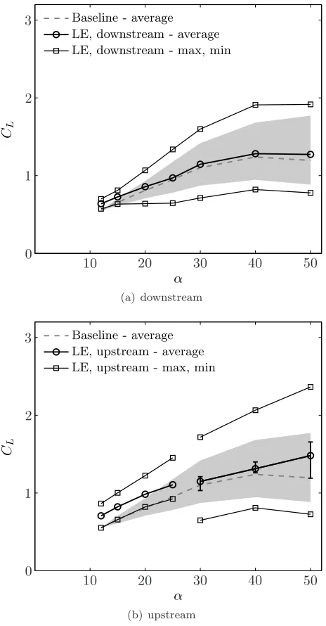
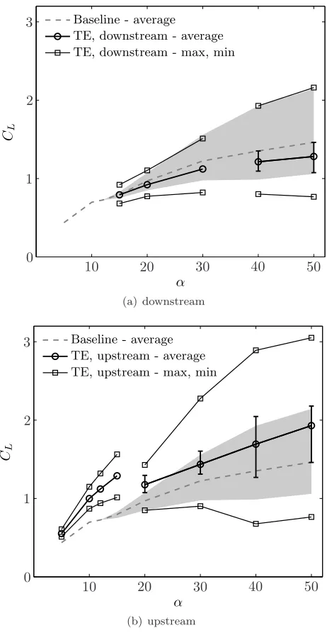
Figure 3.3 shows the lift coefficient with actuation at the leading edge directed downstream (top) and upstream (bottom). In each figure, the uncontrolled flow (baseline) is overlaid in grey with its average in dashed grey and its maximum and minimum bounding the shaded region. Squares show the minimum and maximum of the lift signal whose overall average is shown in the circles in between. For cases where the lift is not phase locked to the forcing signal, variation in the period-averaged lift (averaged over each actuation period) is also plotted with an error bar.

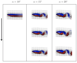
α= 10◦ _{α= 15}◦ _{α= 20}◦

(a) Vorticity flowfield atα= 10◦_{, 15}◦_{, and 20}◦

α= 30◦ _{α= 40}◦ _{α= 50}◦

(b) Vorticity flowfield atα= 30◦_{, 40}◦_{, and 50}◦

of the lift fluctuations. The forced flow exhibits higher maximum lift but also lower minimum lift, below that of the baseline flow. As a result, blowing downstream does not significantly benefit the overall average lift.

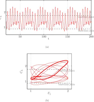
However, when the actuation is directed upstream, the resulting amplification of the unsteady shedding has a more positive effect on the average lift. Forα <25◦_{, the flow locks onto the forcing} 2 ∼3 periods after the actuation is initiated. However at higher α, the flow fails to lock onto the forcing frequency and displays a more complicated limit cycle, with subharmonics of the forcing frequency also excited. An example is shown in Figure 3.4, atα = 50◦ _{where each subharmonic} limit cycle consists of several periods with a different period-averaged lift. Figure3.4also shows the lift as a function of the jet velocity, and shows that the actuation produces the highest lift when Uj is in phase with theCL (maximumCL whenUj is maximum). However, the succeeding period becomes slightly out of phase and the lift decreases. Each period within the subharmonic limit cycle is observed to be associated with a particular phase shift,φ, between the forcing signal and the lift, yielding a particular period-averaged lift. The actuation period associated with the highest average lift is plotted in a thicker line. At eachα, there is a particularφ, resulting in the highest average lift over an actuation period. If the feedback allows us to accordingly adjust the frequency of actuation to phase lock the flow at theseφ, then we could repeatedly produce the highest average lift period. This feedback design will be revisited later.

It might be counter-intuitive that upstream actuation at the leading edge achieves such a lift enhancement and performs better than downstream actuation. However, experiments at Reynolds number of the order of 3×105_{byRullanet al.(2006) demonstrated that unsteady blowing upstream,} parallel to the chord at the leading-edge of a sharp-edged, circular arc airfoil at variousαbeyond stall leads to averaged pressure distribution that resulted in higher lift than that of the baseline flow. They achieved lift increase as high as 30% with momentum coefficient of Cµ′ =Cµ/sin(α)≈1%,

α CL

Baseline - average LE, downstream - average LE, downstream - max, min

10 20 30 40 50

0 1 2 3

(a) downstream

α CL

Baseline - average LE, upstream - average LE, upstream - max, min

10 20 30 40 50

0 1 2 3

(b) upstream

t CL

baseline,min baseline,max

50 100 150 200

1 2

(a)

Uj

CL

baseline,min baseline,max

1 2

1 2

(b)

3.2.2.2 Trailing-edge actuation

In Figure3.5, the lift performance of the open-loop actuation at the natural shedding frequency at the trailing edge is investigated in a similar manner as in Figure3.3. Blowing downstream exerts a negative effect on the average lift, yielding a lower minimum lift than that of the baseline flow with a similar maximum lift. However, when the forcing is directed upstream, the forced flow displays a significant lift enhancement. The forcing excites the vortex shedding cycle even forαbelow the Hopf bifurcation. Forα≤15◦_{, the flow locks onto the forcing after 2∼3 periods. However, forα≥20}◦_, the subharmonic resonance is excited. This is similar to the observation with upstream blowing at the leading edge, but the subharmonic resonance is excited at a lower α for the trailing-edge actuation than that for the leading-edge actuation.

Each period within the subharmonic limit cycle is again observed to be associated with a partic-ularφ, resulting in a particular period-averaged lift. We denote theφ associated with the highest period-averaged lift at each αas φbest. Particularly atα= 30◦, 40◦, and 50◦, φbest was observed to be approximately −0.25, −0.05, and 0.0 radians, respectively. For trailing-edge actuation, the period-averaged lift at high α is, in many cases, greater than the maximum lift occurring in the baseline flow. This suggests a greater potential for the trailing-edge feedback actuation to sustain the flow with the highest period-averaged lift. Consequently, we would obtain a phase-locked flow that has an average lift as high as the maximum lift of the baseline flow (or even higher).

that the actuation near the trailing-edge on the upper surface, 0.8cfrom the leading edge, improves lift and drag characteristics by manipulating the circulation of the TEV.

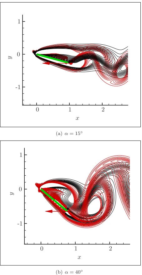
In order to understand the lift-enhancing mechanism of upstream actuation at the trailing edge, we compare the vorticity contours at the time of maximum lift for the cases of baseline and upstream actuation at the trailing edge, for 40◦ _{in Figure 3.8. Actuation feeds extra circulation to the TEV} which induces a stronger downwash near the trailing edge. As a result, the vortex structure on the suction side is pulled down closer to the plate and the backflow near the trailing edge is reduced. Particularly atα= 40◦_{, this delays the interference of the newly forming TEV with the LEV residing} on the suction side. It also lengthens the duration over which the vortex structure is formed from the leading edge. These results also agree with the observations that the period associated with the highest lift within a subharmonic cycle in Figure3.5(b)has a longer period than that of the baseline flow. This might indicate that there exists a forcing frequency belowωn, at which the flow becomes phase locked to the forcing at a higher lift than that of the baseline flow.

Thus, we next investigate the possibility of the existence of shedding cycles that are phase locked to the open-loop forcing signal. Figure 3.9 shows the lift response to the variation in open-loop forcing frequency for 20◦_≤α≤50◦_{, above which upstream actuation atω}

f=ωn fails to phase lock the flow.

Over a range of frequency belowωn, the flow is phase locked to the actuation with its average lift near the maximum period-averaged lift of the flow actuated at ωf =ωn. As we go deeper into stall by increasingα, the domain of attraction for the phase-locked limit cycle decreases, and finally atα= 50◦_{, actuation failed to phase lock the flow over the range of forcing frequencies considered.} Figure3.10shows the corresponding phase shift,φ, over this range ofωf that achieves a phase-locked flow forα= 30◦_{. Recall that the subharmonic cycle (excited with upstream blowing atω}

φ, closer to φbest with higher average lift. Finally, at ωf/ωn ≈0.87, the actuation is able to lock the flow at the best period achieved with forcing atωn. This indicates that each phase-locked limit cycle of the vortex shedding could be characterized by its frequency and the phase shift, yielding a particular maximum, minimum, and average lift.

If the feedback allows us to adjust the frequency of the actuation accordingly to keep the phase shift between the forcing signal and the lift constant (for example atφ=φbest), we should be able to reproduce the high-lift shedding cycles over a wide range ofα. Thus in order to achieve the desired phase-locked shedding cycle, we feedback lift into the controller, whose details are described in the next section.

3.3

Closed-loop control

Open-loop periodic forcing can lead to limit cycles with a high average lift, but with a decreasing domain of attraction asαincreases. Our goal with closed-loop control is to obtain forced limit cycles with the maximum average lift. This involves stably maintaining limit cycles that are not stable without feedback.

Since the actuated flows with the highest average lift seem to be characterized by a distinct phase shift of the forcing relative to the lift at eachα, we feedbackCLin an attempt to phase lock the flow

at these high-lift states. Direct feedback ofCL with appropriate gain would only allow us to force

α CL

Baseline - average

TE, downstream - average TE, downstream - max, min

10 20 30 40 50

0 1 2 3

(a) downstream

α CL

Baseline - average TE, upstream - average TE, upstream - max, min

10 20 30 40 50

0 1 2 3

(b) upstream

t CL

baseline,min baseline,max

50 100 200

1 2 3

(a)

Uj

CL baseline,max

baseline,min

0 1

1 2 3

(b)

Figure 3.6: Lift with upstream actuation at the trailing-edge at it natural shedding frequency (ωf=ωn), forα= 50◦.

x

y

x

y

0 1 2

-1 0

1

(a)α= 15◦

x

y

0 1 2

-1 0 1

(b)α_{= 40}◦

ωf/ωn

CL

phase-locked limit cycle

0.8 1

1 2 3

(a)α= 20◦

ωf/ωn

CL

phase-locked limit cycle

0.8 1

1 2 3

(b)α_{= 30}◦

ωf/ωn

CL

OL1

phase-locked limit cycle

0.8 1

1 2 3

(c)α_{= 40}◦

ωf/ωn

CL

0.8 1

1 2 3

(d)α= 50◦

ωf/ωn

φ

0.8 0.9 1

-0.4 -0.2 0

Figure 3.10: Trailing-edge actuation: phase shift of the forcing signal,Uj, relative to the lift signal,

CL, for phase-locked flows, over a range of open-loop forcing frequency,ωf (α= 30◦).

U

{

U

(

t

)

Plant

U

(

t

)

C

(

t

)

Controller

φ

ω

φ

ω

C

(

t

)

Figure 3.11: Feedback control configuration.

can be expressed as

CL(t) = a0+ALcos(ωit+θ),

= a0+a1cos(ωit) +b1sin(ωit). (3.3)

Assuming that AL andθ are slowly varying in time, we can estimate a1 and b1 to be the Fourier mode over a moving window,

a1(t) = 2 Ti

Z t

t−Ti

L(t′) cos(ωit′)dt′, (3.4)

b1(t) = 2 Ti

Z t

t−Ti

L(t′) sin(ωit′)dt′, (3.5)

ωi =

2π Ti

. (3.6)

appropriate gain,Kp,

Uj(t) =a0+Kp(a1(t) cos(ωit+φi) +b1(t) sin(ωit+φi)), (3.7)

wherea0is the average value of the outputUj, which can be prescribed as 0.5 to fixCµ= 0.01. We

also adjustKp continuously, such that the rms amplitude ofUjremains steady and similar to that of open-loop control, i.e. Uj varies from 0 to 1.

The configuration of our feedback control is shown in Figure3.11. Lift is fed back to the controller which has two parameters: demodulation frequency,ωi, and the desired phase shiftφi. The controller outputs a sinusoidal Uj that is phase shifted relative to the dominant frequency of the lift signal. The flow system outputs CL, which has a frequencyωo and a phase shiftφo relative to the input signalUj.

IfCL is phase-locked toUj, the frequency ofUjwill always be the same as the frequency ofCL.

However, if the demodulation frequency,ωi is not equal to the frequency of the lift signal, ωo, then φo will be different fromφi (unless ωo=ωi in which case φo=φi). Thus, it is necessary to add an integral part to the algorithm to adjustωi, such that,

ω_ik+1=ωik+β(ωok−ωki). (3.8)

We can adjust ωi until it reaches ωo, and thus obtain the exact desired phase shift and allow the frequency content to be determined only by the flow. Then we have a robust compensator to explore different limit cycles that are phase locked at variousφat different α.

Figure 3.12 investigates the sensitivity of the lift and the frequency of the forced phase-locked limit cycles to the changes in the phase shift, φ at α= 40◦ _{and 50}◦_{. Feedback was able to phase} lock the flow at any desired phase shift after 2 ∼5 periods over a wide range of−0.5≤φ ≤0.5. At α = 40◦_{, as shown in figure 3.12(a), FB}

even higher-lift limit cycle was achieved near zero phase shift, resulting in as high as 83% increase in the average lift coefficient. A broad range of φ (-0.28≤ φ ≤0.06) resulted in average lift that was higher than the maximum lift of the baseline flow, that is more than 45% in the average lift enhancement. Atα= 50◦_{, the highest average lift occurred near zero phase shift, and over a range} ofφ,−0.3≤φ≤0.16 the actuation achieved at least 25% enhancement over the average lift of the natural flow. At bothα’s, a larger range of negative phase shift contributed more to lift enhancement than the positive phase shift. Particularly atα= 40◦_{, there was a sharp decrease in the lift after} φ = 0.06 whereas the lift decrease was more gradual at the negative phase shift. In other words, having most of the control effort prior to the maximum lift (negative phase shift) does not penalize the average lift significantly. However, having the control peak after the maximum lift (positive phase shift) can significantly degrade the lift performance. Thus, forcing seems more effective as the newly forming LEV is pulled down by the TEV (lift-increasing phase). On the other hand, forcing seems the least effective after the maximum lift occurs; when the LEV sits closest to the plate and is pushed away by the growing TEV (lift-decreasing phase). Asφapproaches 0.5 or -0.5 (out of phase), the forced flow results in the average lift similar to that of an unforced flow, but with a slightly smaller magnitude of oscillation in lift coefficient. This sensitivity of the lift to the control effort during different phases of the vortex shedding cycle (particularly lift-increasing and -decreasing phases) will be revisited in the context of optimized waveform in the next Chapter.

Recall in Figure3.9(c), we observe a very small domain of attraction nearωf≈0.8 for the phase-locked limit cycle and the resulting limit cycle has a positive phase shift,φ≈+0.3. However, the phase-locked limit cycles achieved by this feedback have a wide range of frequencies, varying from 0.8 to 0.95 with the corresponding phase shifts ranging from−0.5 to 0.5. These limit cycles were not achieved by any of the forcing frequencies of the open-loop control in Figure3.9(c). The feedback algorithm results in phase-locked limit cycles that are not attainable by the open-loop forcing.

lift cycle during earlier periods, with its phase shift closer to φbest. But after a few periods, φ drifts away fromφbest and the flow eventually locks onto the lower average lift cycle. On the other hand, the feedback compensator prevents φ from drifting away and sustains the phase at φbest producing higher average lift than the open-loop control. Thus, we can conclude that this feedback algorithm stabilizes the limit cycle with a significant lift enhancement that cannot be obtained with the open-loop control.

To ensure that the feedback is still required to sustain the achieved phase-locked limit cycle, FB1 is investigated further. Feedback is turned off after the phase-locked limit cycle has been achieved for a long time, and the forcing signal is continued with the open-loop forcing at a fixed frequency, ωf, as shown in Figure3.14. This behavior of unstable phase relationship has also been shown with a open- and closed-loop control model of an oscillating cylinder wake byTadmoret al.(2004). Notice that when the forcing signal is continued with the actuation ofωf =ωo,OL1, the flow drifts back to

the previous open-loop limit cycle. When it is continued with actuation oscillating atωf=ωo,FB1,

FB1

CL

ωo

/

ωn

φo

-0.5 -0.2 0 0.2 0.5

0.8 0.9 1 1 2 3

(a)α= 40◦

125% baseline,ave CL

ωo

/

ωn

φo

-0.5 -0.2 0 0.2 0.5

0.8 0.9 1 1 2 3

(b)α_{= 50}◦

t CL

100 150

1 2 3

Figure 3.13: Comparison between open-loop control case (–), that phase locked the flow at the highest averageCL (denoted as OL1 in Figure3.9(c)), and the corresponding feedback control case (–) (denoted as FB1in Figure3.12). Forcing frequency of this open-loop control is denoted asωf,OL1,

and the average output frequency ofCL of the feedback control is denoted asωo,FB1.

t CL

open-loop control feedback control

100 200 300

1 2 3

(a)ω_f=ω_o,FB1

t CL

open-loop control feedback control

100 200 300

1 2 3

(b)ω_f =ω_f,OL1

Chapter 4

Optimized waveform at

Re

= 300

4.1

Numerical Method

Simulations of flow over a two-dimensional flat plate atRe= 300 and an angle of attack of 40◦ are performed with the immersed boundary projection method combined with a vorticity-streamfunction multi-domain technique (Taira & Colonius,2007;Colonius & Taira,2008). We model the actuation as unsteady velocity boundary conditionsφ=Ujapplied at the control point (trailing edge)C.

For clarity, the incompressible viscous flow equations ((2.9) and (2.10)) is presented here in operator form by (4.2) and (4.3). The control is implemented as a velocity boundary conditions φ(x, t) applied at the actuation pointsC shown in Figure4.1. In the case of our interest, control is a function only of time, andφ(x, t) =φ(t) =Uj(t), which is the prescribed velocity at the actuation point.

Three vector fields are first defined: the flow state q, the flow perturbation state q′, and the adjoint stateq∗:

q= γ ˜ f

, q′=

γ′ ˜ f′

, q∗=

γ∗ ˜ f∗ . (4.1)

whereq is a vector of flow variables and the motivation for introducingq′ anadq∗ will be obvious later in the control derivation.

For clarity, all differential equations are written in operator form in this section. Incompressible viscous Navier-Stokes equation can be written in operator form as

N (q) =Fφ (4.2)

where the (nonlinear) operatorN (q) is

N (q) =

dγ dt +C

T_ET_f˜+βCT_Cγ−CT_n(q)−bc

γ

ECs

. (4.3)

γ is the discrete circulation and ˜f = [ ˜fx f˜y]Tis a vector of surface forces on the Lagrangian body

for the actuation points. The vector F = [Fγ F_f˜]T allocates the control action. Thus Fγ =0

and F_f˜ has a single non-zero entry that corresponds to the actuator location associated with the appropriate element of the surface force, ˜f.

Ω α

C

U∞

φ

Figure 4.1: Schematic of upstream actuation at the trailing-edge.

4.2

Adjoint-based Optimization

We compute the optimal control over a time horizon, using the receding-horizon approach (Bewley

et al.,2001). The procedure is simlar to previous studies (Bewleyet al.,2001;Wei & Freund,2006) and is only outlined briefly here.

4.2.1

Adjoint-based Optimization: Cost Functional and Sensitivity

To maximize lift, we define a cost functional to be minimized

J =−

Z t1

t0 Z

Ω ˜ f2

y(φ(t), x, t)dx dt+Cw

Z t1

t0 Z

C

φ2_{(t)dx dt, (4.4)}

wheret0andt1 are the start and end times of the optimization horizon and Ω is the surface of the body (see Figure4.1). φis the control input, in this caseφ(t) =Uj(t). Again, ˜fy is they component

of forces on the plate calculated in the immersed boundary projection method. The first term is the total squared lift over the optimization horizon. The second term penalizes the actuator amplitude in order to keepCµ to a value commensurate with the open-loop control discussed previously. The

control weight,Cw, is determined by trial and error and is held fixed throughout the optimization.

perturbation φ′ _{to the control φ. The quantity J}′ _{may be defined by a limiting process as the} Fr´echet differential (Vainberg,1964) of the cost functionalJ with respect toφsuch that

J′,lim

ǫ→0

J(φ+ǫφ′_)−J(φ)

ǫ ,

Z t1

t0 Z

Ω

DJ(φ)

Dφ φ

′_{dx dt. (4.5)}

In the case of our cost functional as in (4.4), this sensitivity of the cost functionalJ′ resulting from a control perturbationφ′ _{may be written as}

J′=−

Z t1

t0 Z

Ω

2( ˜fy(φ(t), x, t)) ˜fy′dx dt+Cw

Z t1

t0 Z

C

2φ(t)φ′dx dt, (4.6)

where ˜f′

y is the Fr´echet differential ofφas defined in the following subsection.

4.2.2

Adjoint-based Optimization: Formulation

Now consider the linearized perturbationq′ to the flow q resulting from a perturbationφ′ _{to the} controlφ. The quantityq′ _{may be defined by the limiting process of a Frechet differential such that}

q′ ,lim

ǫ→0

q(φ+ǫφ′)−q(φ)

ǫ . (4.7)

We takeq′to be the still unknown perturbation to a solutionqof the flow equation due to a control perturbationφ′_{. Mathematically, this means that}

N (q+q′) =F(φ+φ′) (4.8)

where the notation for the term on the right-hand side indicates that the vector F multiplies the scalarφ+φ′. Linearizing (4.8) inq′, or equivalently taking the differential of the governing equation (4.2), yields

The operatorN ′_(q)q′ _{is linear in q}′_{, thoughN} ′_{(q) is itself a nonlinear function ofq. Using the} same Inner product defined as (A.4) in AppendixA,

hc, di=

Z t1

t0 Z

γc·(CTC)−1·γddx dt+

Z t1

t0 Z

˜

fc·f˜ddx dt, (4.10)

c= _γ c ˜ fc

, d=

_γ d ˜ fd , (4.11)

consider the following identity

hN ′(q)q′,q∗i=hq′,N ∗(q)q∗i+b, (4.12)

where the operationN∗(q)q∗is a linear operation on the adjoint fieldq∗and the operatorN∗(q) is itself a function of the solutionqof the Navier-Stokes problem. The boundary termbis eliminated by choosing appropriate boundary and initial conditions for the adjoint problem. Causality eliminates the time boundary term at the inital time t = t0: there can be no perturbation to the flow (i.e.

q′ = 0) due to the control before the control is applied. The condition at the end time t = t1 is eliminated by simply starting withq∗_{= 0 att=t}

1and solving the adjoint system backward in time. Integration by parts may be used to move all differential operations fromq′_{on the left-hand side of} (4.12) toq∗ on the right-hand side, resulting in the same adjoint operator derived in Appendix A:

N∗(q) =

₋dγ∗

dt +C

T_ET_f˜∗_+βCT_Cγ∗_−(CT_C)n

L(γ0)Tqa

ECf˜∗

. (4.13)

We can now choose a source termF∗for our adjoint system

so that the adjoint solution provides the gradient DJ/Dφ. We start by substituting (4.9) and (4.23) into (4.12) withb= 0, which becomes,

hFφ′,q∗i=hq′,F∗i. (4.15)

Comparing (4.15) with (4.6) and (4.5), we would like to obtain

hq′,F∗i=

Z t1

t0 Z

Ω

2( ˜fy(φ(t), x, t)) ˜fy′dx dt, (4.16)

so that

hFφ′,q∗i=

Z t1

t0 Z

Ω

DJ(φ)

Dφ φ

′_{dx dt+C}

w

Z t1

t0 Z

Ω0

2φ(t)φ′dx dt. (4.17)

The adjoint source termF∗ that gives (4.16) is

F∗γ = 0, F∗_f˜_x = 0, F∗_f˜_y = 2( ˜fyφ(t), x, t), (4.18)

and (4.6) and (4.5) becomes,

J′, Z t1

t0 Z

Ω

DJ(φ)

Dφ φ

′_{dx dt=}Z t

1

t0 Z

Ω0

(2Cwφ(t) +F_f˜·f˜∗)φ′dx dt. (4.19)

Then, by (4.17) the gradient becomes

g(φ) = DJ(�