Specification and Construction of Control Flow Semantics : a generic approach using graph transformations

(1)

Specification and Construction

of

Control Flow Semantics

a generic approach using graph transformations

R.M. Smelik

Master of Science Thesis

Enschede, 26th January 2006

Twente Research and Education on Software Engineering ()

Dept. of Electrical Engineering, Mathematics and Computer Science University of Twente, the Netherlands

(2)

(3)

Abstract

The semantics of programming languages lack a formal, standardized specification lan-guage. We focus on control flow semantics and propose a graphical specification framework for these semantics, consisting of three elements: a graphical control flow specification lan-guage, a rule-based approach for constructing flow graphs and transformations from the former to the latter.

In this thesis we introduce a control flow specification language () with which a language designer can specify the control flow semantics of all constructs that are featured in the programming language he or she designs. A control flow specification inconsists of a set of specification graphs that adhere to themeta-model.

We also presents a structured, rule-based approach for constructing a flow graph () for a program written in a particular programming language. In this approach, we use graph transformations to transform an abstract syntax graph representation () of the program into a . Such a graph transformation system consists of a set of programming language specificconstruction rules.

(4)

(5)

Introduction

Like natural languages, all programming languages have a grammar, which specifies the legal syntactical structures of the language. This grammar is typically specified in a formal notation called Extended Backus-Naur Form ( [9]). Besides a syntactical structure, a programming language has semantics. The semantics of a programming language, contrary to the syntax, is typically specified informally, using natural language. The absence of a formal specification language for the semantics of programming languages might in some cases introduce ambiguity in the interpretation of the semantics of a programming construct. But the main problem is that it makes automated reasoning or correctness proving of, for instance, refactoring operations more difficult.

These problems also play a role in Model Driven Architecture () [12]. In the approach several, preferably automatic, transformation steps are developed in order to transform a platform independent specification model of a system to a model which depends more on a specific platform or technology. This process ideally ends at the level of an executable model. In order to assure the correctness of any of these transformations, we need a formal specification of the semantics of both the source language and the target language of the transformation step. These are then used to prove that the transformation step preserves the semantics of the source model.

It is therefore clear that it is desirable to have a standard, formal specification language for the semantics of programming languages, comparable to thestandard that we have for the syntax of languages.

This thesis will introduce a specification language that focusses on a subset of the se-mantics of programming languages, namely thecontrol flow semantics. To put it simply, control flow defines theorderin which individual operations in a program are executed. The control flow semantics of a programming construct is described in terms of the influence this construct has on this execution order in a program.

1.1 Goal

The goal of this thesis is:

(8)

2 Introduction

1.2 Approach

Our research has resulted in a framework for formal specification of control flow semantics, consisting of:

1. A control flow specification language (the main goal of this research project);

2. A flow graph construction approach;

3. Transformations between the above two elements.

All the elements of this framework have been implemented, using graphs and graph transformations. Below, we give a brief introduction to each element. The coming chapters will treat them in far more detail and present an instantiation of this framework for our example programming language.

1.2.1 Control flow specification language

The purpose of our control flow specification language (to which we will often refer as) is for a language designer to be able to formally specify the control flow semantics of the programming language he or she is designing. The most important requirements for  are the following:

1. The language should have formal semantics;

2. The language should be programming language independent, i.e. generic;

3. A control flow specification for a particular programming language inshould have a close relation to the syntax of the programming language;

4. The language should be powerful enough to be able to specify all control flow semantics for any imperative programming language (including object-oriented languages with imperative programming constructs).

When we specify the control flow semantics of a particular programming language in , we design acontrol flow specificationfor each individual programming construct in the programming language. Such a control flow specification states the influence the construct has on the flow of control of any program that features this construct. Together, this set of control flow specifications forms a specification of the control flow semantics of the entire programming language.

Regarding requirement 1, ouris based on the mathematicalgraphdatatype: control flow specifications inare graphs which adhere to themeta-model. The meta-model consists of programming language independent (requirement 2) graph elements (i.e. nodes and edges) we use to denote control flow in a specification.

(9)

Introduction 3

Regarding requirement 3, the close relation with programming language syntax is re-alised by the fact that we use a graph representation of abstracted syntax of a particular programming language construct as the base of a control flow specification for this construct. For this base graph we specify the control flow of the programming construct with (graph) elements present in themeta-model.

It is not straightforward to show that requirement 4 is fulfilled by. At the end of this thesis, we present a critical evaluation of the applicability ofto imperative programming languages.

1.2.2 Flow graph construction

In the previous section we introducedin which we can specify the control flow semantics of aprogramming language. We now consider constructing the control flow of aprogramwritten in some programming language.

In our framework, we represent the control flow of a program as aflow graph. For program analysis and measurements of the structural complexity of a code fragment, programs are often represented as flow diagrams or flow graphs [5]. The properties of these graphs (like the number of independent paths in a flow graph) can provide the necessary information for this kind of analysis [20].

There are many possible ways of modeling flow graphs, ranging from detailed and accurate (with respect to real program execution) representations to abstract representations that are more suitable for (mathematical) analysis of complexity properties. We use a detailed flow graph model, which is based on an abstract graph representation of syntax to which we introduce control flow information. We present an elaborate flow graph meta-model that accommodates for the different types of control flow we discern.

We present a structured, rule-based way of introducing control flow information. For each type of programming construct, we design a rule that decorates its abstract syntax representation with our representation of its control flow semantics. We apply a set of these rules in order to transform an abstract syntax graph representation into our flow graph representation.

The abstract syntax representation we use is a graph, i.e. anabstract syntax graphand, of course, our flow graph is also a graph. Because of this we are able to use a transformation technique known asgraph transformations[15]. When using graph transformations, we have a graph grammar or graph production system, which consists of a set of graph production rulesand astart graph. The start graph is, in this case, an abstract syntax graph representation of some program (fragment) for which we want to construct a flow graph. This program is written in a specific programming language. For each programming construct that is featured in this language, the set of production rules provides a rule that transforms a matchingpart of the abstract syntax representation into a partial flow graph. In other words, for each type of statement we have a rule that introduces the control flow information of this statement to the abstract syntax graph of the program that features this statement. After applying all matching rules to the abstract syntax start graph, we end up with a completed flow graph.

(10)

4 Introduction

this case study, we have developed and applied several different approaches, before coming to the final approach and meta-models that we use in this thesis.

1.2.3 From specifications to construction rules

As we mentioned earlier, we present as a means for a language designer to formally specify the control flow semantics of a programming language. A language designer specifies for each programming construct of the language he or she is designing the control flow semantics as a control flow specification. This results in a set of formal specifications that can accompany the formal syntax specification of the programming language.

We also mentioned the purpose and benefits of representing a program as a flow graph and having a structured way for constructing such graphs. As follows from the case study, designing flow graph construction rules by hand is time-consuming and not a trivial task. Fortunately, graph transformations can aid us here (again).

Our control flow specification framework includes a set offlow graph meta-rules: graph production rules that transform graphs intro graph production rules. The source graphs of these meta-rules are a set of hand-designed control flow specifications in. The production rules that result from the application of these meta-rules are the corresponding flow graph construction rules. Therefore, there is no need to design these flow graph construction rules by hand.

1.2.4 Running example: the Java programming language

To provide concrete examples for bothas our flow graph construction approach, we have chosen for the Java programming language [19], a modern and widespread programming language. We have composed an abstract grammar which features most Java constructs. For these constructs we present a set of control flow specifications in. We also present a corresponding set of flow graph construction rules for these constructs in this thesis, which were generated by our flow graph meta-rules.

1.3 The big picture

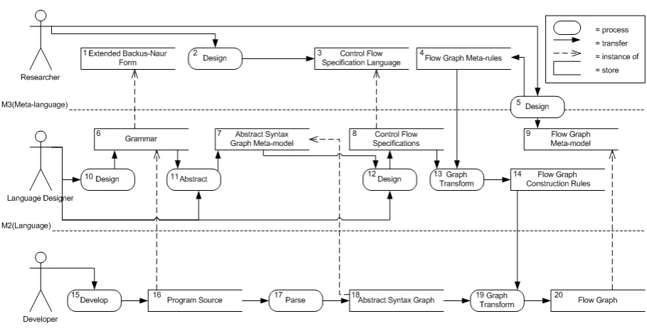
It is time to present an overview of all elements of this research mentioned above (the big picture). For this, we look at Figure 1.1.

This figure features three meta-levels. Level 1 is at the level of program defined in a specific programming language. Level 2 is at the level of a specific programming language, of which a program of course is an instance. Level 3 is at the level of meta-languages, the level in which parts of a specific programming language are defined.

Three types of actors play a role in this figure. We have aresearcherwho designs meta-languages and meta-models. Next we have alanguage designer; he or she designs the syntax and semantics of a specific programming language. And last, we have adeveloper; he or she develops a program in this specific language.

(11)

Introduction 5

Figure 1.1: Overview of the chain of the elements involved in this thesis and the levels on which they reside.

Next he or she specifies the control flow semantics of the language, not in natural lan-guage, but in formal specifications (8) in our control flow specification language (3).

Graph transformations (13) are performed on these specifications using thetool set [14], which applies our designed set of flow graph meta-rules (4). The performed graph transformations result in a set of corresponding flow graph construction rules (14).

Now we examine the role of the developer. The developer writes (15) some program (16) in this new programming language, conforming to the grammar of the language (6). The program is parsed (17), resulting in an abstract syntax graph (18) that conforms to the abstract syntax graph meta-model that is specific for this programming language (7). The abstract syntax graph is input for thetool (19), were the generated set of flow graph construction rules (14) are applied. The resulting transformations result in flow graphs (20) that have been attached to the input abstract syntax graph and adhere to the flow graph meta-model (9).

1.4 Overview

We now give a brief overview of the chapters in this thesis.

Chapter 2 introduces the formal notion of graphs and explains the aspects related to the graph transformation technique and production rule application.

(12)

6 Introduction

Chapter 5 introduces our control flow specification language, the main result of this thesis. As an example for our specification language, we present a large number of example control flow specifications of Java statements.

In Chapter 6 we present our set of flow graph meta-rules that transform control flow specifications into corresponding flow graph construction rules.

Chapter 7 evaluates our control flow specification language and identifies its applicability and limitations.

(13)

Chapter 2

Graph Transformations

This chapter gives an introduction to graph transformations as they are used in this thesis. In the big picture (Figure 1.1) of this thesis, presented in Chapter 1, we have seen that graph transformations are applied to transform control flow specifications into flow graph construction rules (13)1and to construct a flow graph given an abstract syntax graph (19).

Graph transformations are a systematic, rule-based transformation technique. They have a solid research foundation [17] and have many areas in computer science for which they are found suitable to apply (e.g. [15, 3, 7]).

In the next section we introduce the formal definitions of the graphs we use. In the last section, we introduce graph transformations and conclude this chapter with an introduction example to graph transformations.

2.1 Graphs

Graphs are our mainly used datastructure, in fact we represent all components of the frame-work we introduce as graphs. All our graphs conform to the following formal definition.

Definition 2.1.1. [15] A graph is a tupleh_Nod,_Edgi_where • _{Graphs are specified over a global, finite set}_Lab_{of labels;} • _Nod_{is a finite set of nodes;}

• _Edg_{is a subset of}_Nod × _Lab × _Nod_{, i.e. a (finite) set of edges.}

Our graphs aredirectedgraphs, meaning that we discern for each edge asourceand atarget

node. As a result, our edges can only representbinaryrelations (i.e. we have nohyperedges). As follows from the definition, edges are labeled. Nodes are not labeled by definition, but we can have edges with the same source and target node. These edges are calledself-edges

of a node and, for practical purposes, can be considered as the labels of a node (as a result, a node can have several labels). As we use asetof edges, we do not have multiple edges with the same source, target and label (i.e. noparalleledges).

Graphically, nodes are represented as black rectangles and edges as black arrows. Self-edges can be represented as labels of nodes (graphically depicted inside the rectangle), or as arrows with the same start and end node.

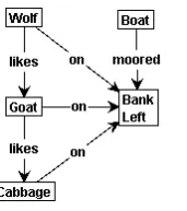
Figure 2.1 shows an example graph. This graph is part of the Ferryman Problem example that will be elaborated in Section 2.2.4. Note that we have represented self-edges as labels of nodes in this figure.

(14)

8 Graph Transformations

Figure 2.1: An example graph that conforms to our definitions.

2.2 Graph transformations

Now that we have made clear what type of graph we use in this thesis, we introduce the graph transformations technique and show how we can apply this technique to our graphs. Agraph transformation system, or graph grammar [17], consists of a set ofgraph productions rulesand a start source graph.

A graph transformation system can transform a graph called thesource graph, into an-other graph called thetarget graph. The target graph is a transformed version of the source graph. What the changes to this source graph are depends on what is specified in the graph production rules that were applied to this source graph.

2.2.1 Graph production rules

A graph production rule consist of two graphs, aleft hand side Land aright hand side R. A production rulep has the form: L→r _R_{. The left hand side} _L _{is matched to (a part of) the}

source graph and the occurrence ofLin the source graph is replaced by R, resulting in the target graph. Thus, the left hand sideLis matched on the source graph and the right hand side specifies elements (nodes or edges) of the matching sub graph (of the source graph) to be preserved, elements to be removed and new elements to be introduced in the target graph. r is apartial graph morphism, which identifies which elements (nodes or edges) in L

correspond to which elements inR. Note that we use the Single Pushout Approach, were in the Double Pushout Approach the correspondence of elements is, among others, identified using acommon interface graphorgluing graph[17].

Matching of a left hand side L of a graph production rule on a source graph G is  -complete.

The technical details of our production rules and how they are applied are treated more thoroughly in [17] and, more specifically, in [15].

The production rules are made up from four different kinds of elements:

Readers The readers are elements that are present in bothLandR. They have to be present in the source graph in order forLto match and are preserved in the target graph. Erasers The erasers are elements present inLbut not inR. Thus, they have been matched in

the source graph but are not found in the target graph, i.e. they are removed.

(15)

Graph Transformations 9

Embargoes The embargoes (or negative application conditions) are neither present inLand

Rbut are in fact an extension to standard graph transformations [15]. These elements have to be absent in the source graph and in a matching of Lon the source graph for the production rule to apply.

We give an example application (Pushout) of a graph production rule to a graph in Figure 2.2. The matched nodes and edges in the source graph are depicted bold. By comparingL

andRwe can see that a node and two edges are erased by this production rule. Note that the representation of the negative application conditionmooredinLis technically incorrect. In practice, after a match ofLhas been found in the source graph, the negative application elements are added to this matching graph. Only when this extended matching graph does not (again) match the source graph the rule applies.

Figure 2.2: An application of a graph production rule to a graph.

In our graphical presentation of graph production rules, the left and right hand side are combined in a single graph. To discern the four types of rule elements, each element has a distinct color and form, listed below. Figure 2.3 shows the combined version of the graph production rule presented in Figure 2.2.

Readers Readers are presented as black rectangles and arrows;

Erasers Erasers are presented as dashed, blue (darker gray in black and white presentations) rectangles and arrows;

Creators Creators are presented as bold, green (light gray in black and white presentations) rectangles and arrows;

Embargoes Graphically, they are represented by bold, dashed, red (dark gray in black and white presentations) rectangles and arrows.

(16)

Figure 2.3: An example of the graph production rule depicted withLandRcombined.

x::= a|_x _p _x|_x._x|_x ∗ |_?

The Kleene star (∗_{) matches any number of subsequent edges that match the path}

ex-pression that is left to the operator (the direction of the edges is of course relevant). The choice-operator (|_{) matches a path that matches the path expression left of the operator or the}

path expression right of the operator. The path construction operator (.), matches a path that matches the path expression on the left side of the operator followed by the path expression on the right side (the direction of the edges is again relevant). The wilcard operator (?) matches an edge with any label.

Another operator we often use is the equality operator=which can be the label of a creator or embargo. When it is used as the label of a creator, itmergesthe two nodes it connects to one node, which receives all incident edges of the original nodes. When it is used as the label of an embargo, it states that the two nodes it connects may not be matched to the same node for a matching to be valid. This is sometimes useful, as the matching of elements in the production rule on elements in the source graph can be non-injective (e.g. two nodes in a production rule may be matched onto one node in the source graph).

2.2.2 Rule applications

In a graph transformation system, a set of graph production rules are applied to a start source graph. After each application, the original start graph will be somewhat changed (i.e. transformed). This transformation process typically continues until none of the production rules are applicable anymore to the changed intermediate graph; we can then say that the transformation is complete.

However, at any moment during the transformation process, several rules may apply to the intermediate graph. We can choose to apply one of these rules arbitrarily or explore all applications. This results in a tree-like structure of rule applications and resulting inter-mediate graphs. Because we check each interinter-mediate graph on isomorphism with all other intermediate graphs and connect rule application paths when they result in isomorph result-ing graphs, a tree-structure is not suitable. We represent rule applications usresult-ing a Labeled Transition System (), in which each node is an intermediate graph (the root node is that start graph) and each edge represents a rule application (and is labeled with the name of the rule).

(17)

to a different final graph. When this is the case, the order in which the applicable rules are applied to the intermediate graph influences the resulting final graph.

In our case this is not desirable. We normally design production rules, which will eventually lead to the same target graph, independent of the order in which the rules are applied. Such rules are calledconfluent.

As the order in which applicable production rules is not important when the rules are confluent, we can explore the rule applications in a linear fashion: for each intermediate graph, one applicable rule is chosen arbitrarily. When the order of the applicable production rules is important, we have to perform afullexploration of the rule applications state space to end up with all possible final graphs.

We have another (primitive) mechanism for guiding the applications of production rules: rulepriorities. When a production rule has been given a higher application priority than other rules, the other applicable rules can only be applied in case the rule with higher priority is not applicable.

2.2.3 Graph transformation tool

For graph transformation, we us the[14] tool, which consists of an editor for creating graphs and graph production rules and a simlator for performing graph transformations.

2.2.4 Example: The Ferryman Problem

As an introduction example to graph transformations we consider a classical problem called the Ferryman Problem. We have a ferryman who wants to transport his wolf, his goat, and his cabbage to the other side of a river. The problem is that he has a boat which is only large enough for himself and one other animal or vegetable. Matters are complicated even more for this ferryman by the fact that his possessions have created their own small food chain: his wolf would very much like to devour his goat, while his goat has an interest in his cabbage vegetable. Both the wolf and the goat behave while the ferryman is there to watch them, but will start eating that what they like the moment the ferryman rows away.

We represent this problem as a graph transformation system. Such a system consists, as mentioned above, of a start graph and a set of graph production rules. The start graph (Figure 2.4) is the representation of the start scenario of the Ferryman Problem. The river to cross has twoBanks: oneLeftand oneRight(remember, nodes can have several labels which are actually labeled self-edges of the node).

(18)

The ferryman itself has no explicit representation in our graph, as we are only concerned with the position of theBoat. TheBoatcan bemooredon eitherBankor begoing to the other side of the river.

The two animals and the vegetable are represented as nodes labeled Wolf, Goat and Cabbage. As we know, theWolf likestheGoatand theGoat likestheCabbage. All three can be eitheronone of bothBanks or loadedintheBoat. The start graph states that all three areon the left bank and theBoatis moored on this bank too.

The goal of the ferryman is to transport the wolf, goat and cabbage to the other side of the river. The corresponding goal state graph (Figure 2.5) is the mirrored version of the start graph. There are many possible states which are considered a failure. All fail states have in common that either theGoat or theCabbage or both have been devoured by some animal. An example fail state graph is shown in Figure 2.6. Here we see that, although theWolfhas been transported across the river, both theGoatand theCabbageare no more.

Figure 2.5: The goal state of the Ferryman problem.

Figure 2.6: A fail state of the Ferryman problem.

Now that we have treated the graph representations of states of the Ferryman Problem, we treat the set of graph production rules that are part of the graph transformation system for this problem.

The first production rule we treat is theeatrule (this rule was already depicted in Figure 2.3). This rule performs eating actions according to the food chain. We use a simple and standard technique to make this rule more general: we do not match the pairs (Wolf,Goat) and (Goat, Vegetable), but instead only match on the likesrelation between two unlabeled nodes. As the nodes have no labels, the rule matches on any two nodes that are connected with alikesedge. This way, one rule suffices for both pairs in the food chain. Both elements should of course beon the sameBank in order for the eating process to commence. And, another important condition is that theBoatisnotmoored on thisBank, we therefore have an embargo. The result of theeatrule is that one animal or vegetable will be devoured when applying this rule, i.e. erased.

(19)

shown as separate graphs). In thesource graphfor the rule application, the matching nodes and edges are depicted bold. We can see that theeatrule applies to this source graph, as the Boatis moored on the other side of the river, while theCabbageandGoatare left unattended on the left bank of the river. The figure also shows thetarget graph, the state graph that results from the eating of theCabbage. We see that theCabbagenode and his outgoingon and incominglikesedges have been deleted.

Figure 2.7 shows production rules for the four actions the ferryman can perform:

Load This rule loads one possession that is present on the same bank as theBoatismoored in theBoat(itsonedge is deleted and a newinedge is created) and starts the rowing (by creating agoedge) to the other side (an embargo=specifies that the banks may not be the same node);

Unload This rule unloads one possession on to theBank to which was rowed; theBoatis mooredthere too;

Go empty This rule rows theBoatto the other side (again this cannot be the sameBanknode) without loading any cargo;

Arrive empty This rule mores theBoatwithout unloading any cargo (theBoatmust be empty, i.e. there cannot be any nodeintheBoat).

(a) Load (b) Unload (c) Go - empty (d) Arrive - empty

Figure 2.7: The graph production rules for loading and moving the boat.

Figure 2.8 features the somewhat peculiar rulefinal: it consists only of readers, meaning that the source and target graph of an application of this rule will be equal. This rule is used to indicate that the goal has been reached, i.e. if this rule applies to the current state graph, the Ferryman Problem has been solved.

Figure 2.8: The graph production rule that applies when the success-state is reached.

(20)

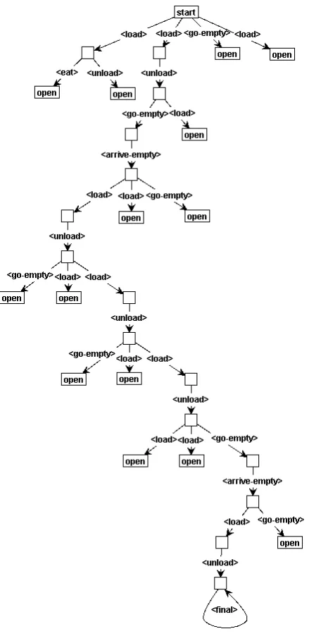
finalrule applies cannot be reached. Rule applications sequences that lead to a state graph in which thefinal rule applies are solutions to the Ferryman Problem. Figure 2.9 shows a (partial) rule applicationin which a sequence of rule applications lead to a graph to which thefinalrule applies. This sequence is a solution for the Ferryman Problem. Exploring any sequence from a state graph labeledopenmight lead to other solutions or failures.

(21)

Chapter 3

Graph Representations

This chapter treats two important graph representations in this thesis: abstract syntax graphs (’s) and the flow graphs (’s). Related to the big picture of this thesis (Figure 1.1), this chapter presents the abstract syntax meta-model (7) and the flow graph meta-model (9) and gives examples of an abstract syntax graph (18) and flow graph (20) for a Java program.

3.1 Abstract syntax graphs

The (context-free) grammar of a programming language is typically specified in (extended) Backus-Naur Form (()) [9]. When parsing the source code of a program written in this language using thegrammar, the result is a concrete syntax tree: a tree structure representing the program’s source, containing all syntactic elements (terminals) of the source as leaf nodes and the non-terminals as intermediate nodes.

Syntactic details are often irrelevant to the control flow semantics of the parsed program. Therefore, as is often done in compilers [21], we use an abstract representation of the concrete syntax. In this representation most syntactic tokens (terminals) can be omitted.

A well-known abstract version of the concrete syntax tree is the abstract syntax tree (). This tree-structure is often enhanced in another pass with extra context information: bindings of used variables to their declarations, unification of labels for labeled statements, etc. These enhanced (or “decorated” [21])’s are in fact no longer trees, butgraphs.

Our abstract syntax representation is also a graph, hence we call it anabstract syntax graph

(). Yet the original tree-structure is still clearly visible in these’s. The non-terminal symbols in the production rules of a programming language grammar appear as nodes of our’s. The syntax tree structure is represented by edges labeledchildbetween parent and child nodes.

Unlike most compiler’s, our’s are not based on a programming language’s grammar, but on an adaptedversion thereof.

An issue with anproduction rule is that the right hand side may feature elements that are optional (enclosed in square brackets). The presence or absence of these elements in a concrete program fragment may affect the control flow semantics of that particular statement. As a concrete example, consider the if-statement that is featured in the Java programming language. The control flow semantics of this statement depends on whether the optional else-part is present. Therefore, when considering the control flow semantics of the if-statement, we actually discern two different statements: an if-then-statement and an if-then-else-statement.

(22)

16 Graph Representations

we combine using the standard or-operator (denoted by|). In other words, we introduce new non-terminals for each variation of a statement due to optional parts. This actually means that we use plainwithout extensions for our abstract syntax.

When considering the if-statement in Java again, our abstract syntax has the following production rules (we use<and>to indicate terminals):

Statement ::= IfStatement | .. | .. IfStatement ::= IfThen | IfThenElse

IfThenElse ::= <IF> <LPAR> Expression <RPAR> Statement <ELSE> Statement

Appendix A presents an abstract, plain , grammar we have composed for a large portion of the Java programming language (based on thegrammar presented in [6]).

We represent the non-terminals in our abstract syntax as nodes in our abstract syntax graph. Thus, the name of a non-terminal is represented as the label of the corresponding node.

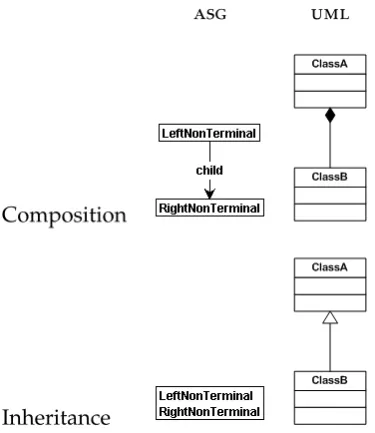
Often, the left hand side of a rule evaluates to one or more non-terminals. There are two possible ways of representing this in our abstract syntax graph, which are similar to two concepts that feature object-oriented programming:compositionorinheritance. If we use composition, the left hand side non-terminal is represented as the parent node and the right hand side non-terminal(s) as child node(s). If we use inheritance, we use the fact that a node can have several labels (represented as self-edges of the node), as we saw in Chapter 2. The left hand side and right hand side non-terminal both appear as labels of the node. Table 3.1 compares both concepts in’s to the correspondingconcepts.

 

Composition

Inheritance

Table 3.1: Composition and inheritance for representing abstract syntax, compared to the correspondingconcepts.

(23)

Graph Representations 17

1 i f ( x >= 5 )

2 x = 0 ;

3 e l s e

4 x = x + 1 ;

Listing 3.1: Example of an if-then-else-statement in Java.

in the grammar above). In this thesis, we make arbitrary choices for using composition or inheritance.

As an example, the IfStatementrule for Java, presented above, is represented using inheritance: an abstract syntax node, labeled IfStatement, also features the label IfThen or IfThenElse(depending on whether it features an else-part).

Beside the tree-structure parent-child relations, represented by child edges, the syntax representation is decorated with additional information. We annotate the relations between parent and child syntax nodes with edges with labels that explain the role of a child syntax node with respect to its parent. We introduce these annotations to our abstract syntax rules using the following notation: label:NonTerminal. Taking Java as an example again, ourrule for the if-then-else-statement in Java therefore becomes:

IfThenElse ::= <IF> <LPAR> condition:Expression <RPAR> thenPart:Statement <ELSE> elsePart:Statement

In our graph representation, an IfThenElsenode has an edge labeled conditionto its Ex-pressionchild syntax node, an edge labeledthenPart to its then-part Statementsyntax node and an edge labeledelsePartto its else-partStatementsyntax node.

Figure 3.1 shows the abstract syntax graph representation for if-then-else statements in Java. Note that in this representation, terminals likeifandelse and parentheses are not present.

Figure 3.1: The abstract syntax graph representation of theIfThenElsestatement.

(24)

Figure 3.2: An abstract syntax graph of the code fragment in Listing 3.1.

3.1.1 Generic meta-model

As we saw in the big picture (Figure 1.1), an abstract syntax graph conforms to a language-specific abstract syntax model (7). All language language-specific abstract syntax graph meta-models adhere to a prescribed structure. We have specified this structure in agenericabstract syntax meta-model, specific abstract syntax graph meta-models are specializations of this meta-model.

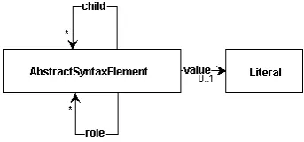
The generic abstract syntax meta-model (Figure 3.3) specifies that an AbstractSyntaxEle-ment (i.e. any node representing a non-terminal) can have any number of children (child) and any number of annotated role edges for these children. The number ofchildedges and annotated role edges need not coincide: achildedge is mandatory for any child of an abstract syntax element, but the annotated roles are optional.

AnAbstractSyntaxElementcan optionally have avaluerelation with a literal value terminal. For instance, aBooleanLiteralin Java has avaluerelation with either theTrueor theFalsenode.

Figure 3.3: The generic abstract syntax meta-model.

(25)

such graphs for the abstract syntax grammar we composed for Java (see Appendix A).

3.2 Flow graphs

Control flow information describes the order in which the individual, atomic, instructions of a program are executed. Most statements are executed in the order they appear in the program’s source code, i.e.sequentialcontrol flow.

However, some statementschangethis sequential flow of control. These statements are often called control statements. They do not perform calculations or change the program’s state, but determine the order of execution for a group of sequential statements. Most control statements depend in their execution on the value of an associated condition. These statements thereby introduce branches in the program’s execution. Depending on the value of the condition one of these branches is executed, i.e.conditional branchingcontrol flow.

Most languages feature another group of statements that disrupt the control flow of a program. The statements perform local (within the method) or in some cases non-local, unconditional jumps. The most (in)famous example is thegoto _{statement [4], that is}

fea-tured in many programming languages. In Java, these statements are referred to as abrupt completion statements. We refer to this type of control flow asabrupt completioncontrol flow. The flow of control in a program is often shown graphically in control flow diagrams or graphs, where arrows or edges indicate how the control is transferred between statements, which are often presented as rectangles or nodes (e.g. [5]). There are many possible ways of modeling flow graphs, ranging from detailed to abstract. Figure 3.4 shows two examples of abstract models of the control flow of Listing 3.1: a flow diagram and a control graph (see [20]). In these figures, the numbers are related to the line numbers of the corresponding listing.

(a) Flow diagram (b) Control graph

Figure 3.4: Examples of control flow diagrams and graphs of Listing 3.1.

(26)

3.2.1 Meta-model

Figure 3.5 presents our flow graph meta-model. We have developed this meta-model during the case study we have performed on designing flow graph construction rules for Java.

Figure 3.5: The flow graph meta-model.

FlowElement

We consider all abstract syntax elements with control flow semantics to be FlowElements. For each FlowElement, we denote which element is executed when control is transferred to this FlowElement (i.e. its entry) and which element represents the end of the FlowElement’s execution (i.e. its exit). Thus, eachFlowElementhas one entryand one exitedge. The target of these edges can be the FlowElement itself, another FlowElement (most likely some sub statement) or aFlowConnector.

The auxiliary nodes FlowConnector, Branch andAbort inherit from FlowElement. As we have seen in Table 3.1, this means that these auxiliary nodes also feature aFlowElementedge and have anentryandexit, which are defined as self-edges of the auxiliary nodes.

FlowConnector

FlowConnectors serve as connection points for control flow in flow graphs and have no semantics of their own.

Sequential control flow

(27)

Conditional branching control flow

Conditional branching has a more complex representation in our flow graphs. We represent each possible branch with an auxiliaryBranchnode. ABranchhas several possible edges:

branch Indicates at which statement the conditional branching originates;

condition Indicates the conditionFlowElementthat results in the actual value for the condi-tional branching;

branchOn Indicates the literal value to which the condition should evaluate if this branch is to be taken;

branchDefault Indicates that this branch is taken if no other branch can be taken;

flow Indicates to whichFlowElementcontrol is transferred upon taking this branch.

AbranchDefault edge is used when we have the specialdefaultcase with, for instance, switch-statements in Java, it excludes a branchOn edge. From a FlowElement that features conditional branching we have abranchedge to each possible branch (Branch). For example, branching on a Boolean condition is represented by two Branches, one ontrueand one on

false. The statement from which this branching originates has abranchedge to each of the Branches.

Conditional branching and sequential control flow are mutually exclusive; a constraint onFlowElements is that they can have an outgoingflowedge or one or more outgoingbranch edges, but not both types of edges.

Abrupt completion control flow

Abrupt completion is the most complex form of control flow. The precise details on abrupt completion are treated in Chapter 4, for now it suffices to explain the representations and constraints for abrupt completion in flow graphs. Abrupt completion is represented by an auxiliary node labeledAbort. AnAborthas several possible edges:

abort Indicates at which statement the abrupt completion control flow originates;

reason Indicates theFlowElementthat causes the abrupt completion control flow;

resumeAbort Indicates at which statement the abrupt completion control flow resumes;

flow Indicates to whichFlowElementcontrol is transferred (analogous toBranch).

(28)

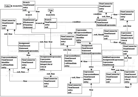
Example flowgraph

As an example flow graph, we consider the Java code fragment in Listing 3.1 again. The abstract syntax graph of this code fragment was presented in Figure 3.2. The flow graph is shown in Figure 3.6, some syntax elements have been grayed out to make the graph more readable. We can clearly see in this graph that the originalhas been decorated by control flow elements. Compared to the models in Figure 3.4 it is clear that our’s are detailed models of the control flow of a program.

Again, the precise details of this flow graph are not important yet. Still, one may wonder where the control flow in this graph starts. Normally, the if-then-else statement is placed in the context of some method that features an ordered list of statements. After execution of the statement ordered before this if-then-else statement, control is transferred to the entry of the if-then-else, in this case theIdentifiernode that is part of the condition. Thus, the statement ordered before the if-then-else would featureflowedge from its exit to theIdentifiernode.

(29)

Chapter 4

Flow Graph Construction Rules

This chapter introduces flow graph construction rules. In the big picture (Figure 1.1) we have seen that flow graph construction rules (14) are applied to an abstract syntax graph (18, see Section 3.1) representation of a program (16) developed in some programming language. The flow graph construction rules are graph production rules (see Chapter 2) that attach a flow graph (20, see Section 3.2) to such an.

Flow graph construction rules construct a flow graph from an abstract syntax graph by introducing elements (nodes and edges) present in the flow graph meta-model (Figure 3.5). There are many possible approaches for this flow graph construction process. The approach we use for flow graph construction and our flow graph meta-model were both developed during an extensive case study on flow graph construction for the Java programming lan-guage.

We first present our flow graph construction approach. Next we illustrate our approach by presenting a large set of example flow graph construction rules for the Java programming language.

4.1 Flow graph construction approach

This section presents our flow graph construction approach. Our approach consist of a number of design choices we have made (during our case study on flow graph construction for Java). We review these choices briefly.

Our approach mainly consist of the following principles:

1. For each type of abstract syntax element, we design one (preferred) or several flow graph construction rules that introduce the necessary control flow elements;

2. Our flow graph construction process operates top-down, starting from the root-node of the flow graph under construction and ending at the level of primitive statements;

3. For each flow element in the graph, we create itsentryandexit(with respect to control flow). Initially, we provide auxiliary flow connectors for these entries and exits;

4. We remove superfluous flow connectors while the flow graph is being constructed;

5. We resolve abrupt completion control flow using a bottom-up resolution process.

(30)

24 Flow Graph Construction Rules

4.1.1 One construction rule per programming construct

Were possible, we designonerule per programming construct. This means that for each con-struct in a programming language, we have a separate production rule that introduces control flow elements to an abstract syntax graph that features that particular type of statement.

We believe that adhering to this standard results in readable and understandable flow graph construction rules, as these rules come close to being a specification of the control flow semantics of a particular statement type (for real control flow specifications, we refer to Chapter 5). Most of the example construction rules for Java (Section 4.2) adhere to this principle and are considered by us to be quite intuitive. In some cases though, we have to break from this principle. An example of this are abrupt completion resolution rules (see Section 4.1.4).

4.1.2 Top-down construction process

Flow graph construction is, in our case, atop-downprocess. By top-down we mean that we start at an abstract syntax node that is defined to be therootof the flow graph we are going to construct. We start flow graph construction at this root node and continue along its abstract syntax children. More concrete, we start by marking the root node as eligible for flow graph construction. The associated flow graph construction rule for the root node removes the marker from this syntax node and marks all its abstract syntax child nodes as eligible. We represent this marking by introducing or removing a self-edge labeledbuildto aFlowElement. Flow graph construction rules for children of the root node match on thisbuildto be present. This way, the application of the flow graph construction rules is ordered top-down.

Figure 4.1 shows how in a flow graph construction rule thebuildmarker is passed on. We have a parent syntax node, for which the marker is removed, andnchild nodes, for which markers are introduced.

Figure 4.1: The top-down flow graph construction process illustrated.

4.1.3 Flow connectors

(31)

Flow Graph Construction Rules 25

The control flow of a parent flow element is, among others, defined as the execution of its flow element children. A result of using a top-down approach is that when a parent flow element is under construction, the control flow of its children has not yet been determined. This fact introduces a problem: the parent flow element production rule introduces control flow that states that one of its child flow elements will be executed upon executing the parent. But, at that time in the construction process, it is unknown where the execution of the child flow element starts (i.e. itsentryis unknown).

Our solution is to provide control flow connector nodes as the (initial) targets for the entryandexitedges of each statement. Parent flow elements can connect their control flow elements to these connector nodes and the child flow elements introduce their internal control flow, starting and ending at their own flow connectors.

During flow graph construction, we introduce entries and exits to each flow element in the flow graph under construction. We connect these edges to auxiliary control flow connectors, represented as nodes labeledFlowConnector. Figure 4.4 shows the generic flow graph construction rule for introducing these elements.

If we were to preserve for every abstract syntax node in a completed flow graph the entry and exit flow connector node, the flow graphs would be somewhat crowded and as a result less readable. Also, in most cases, control flow edges between these flow connectors do not represent actual control flow transfer. In a simulation run of the flow graph these edges would simply be skipped.

We therefore introduce entry and exit flow connectors uniformly to all elements, but we remove superfluous flow connectors during flow graph construction. These flow connectors are merged (see Chapter 2) with other flow connectors or abstract syntax elements, thereby preserving all control flow elements that are connected to the redundant connectors. This merging is performed when the internal control flow structure is known, i.e. when the construction rule associated with the type of flow element is applied.

There are four scenarios in which we consider aFlowConnector obsolete and decide to merge it:

1. A parent flow element’s execution may be defined to start at one of it child elements. In this case, the entry flow connector node is merged with the entry node of the child.

2. A flow element may feature no children (a primitive statement) and define execution to start at the syntax node itself. In this case, the entry flow connector node is merged with the syntax node.

3. A flow element may feature no control flow and therefore can be skipped. In this case, the entry flow connector of the flow element is merged with the exit flow connector.

4. A child flow element may define its exit to be the exit of the parent node. In this case, the exit flow connector of the flow element child is merged with the exit of the parent.

(32)

(a) Scenario 1 (b) Scenario 2 (c) Scenario 3

(d) Scenario 4

Figure 4.2: The different merging operations on flow connectors, corresponding to the four scenarios.

4.1.4 Abrupt completion resolution

Any programming language can feature specific statements that introduce control flow that is not defined with respect to the statement itself or one of its sub statements, but that depends on the context the statement is contained in. The transfer of control they introduce is not a sequential transfer, but a jump to some other statement within the context, thereby terminating prematurely one or, possibly, more statements that enclose this jump statement. We call these statementsabrupt completion statements, as they abruptly complete the execution of one or more enclosing statements.

As these statements disrupt the sequential control flow, flow graph construction rules for these statements are somewhat more involved. The main issue here is that the construction rules have to examine the flow graph context of the abrupt completion statement in order to determine the target statement of the control flow jump that is to be performed. What types of flow elements are eligible to be targets depends on the type of abrupt completion statement.

We refer to the process of finding the correct target flow element for an abrupt completion statement and introducing the abrupt completion control flow to this statement asabrupt completion resolution. The abrupt completion resolution process can be approached in many different ways, as we learned during the case study. As we mentioned, we choose to use a bottom-up resolution process.

When an abrupt completion statement is marked for construction, a corresponding flow graph construction rule introduces abrupt completion flow. As in most cases the target flow element is not immediately known, we use a stepwise resolution process: we propagate an abrupt completion marker element upward in the syntax tree (hence bottom-up) until the target flow element is reached. Next we apply another flow graph construction rule that corresponds both to the type of abrupt completion statement and the type of the target flow element. This rule connects the introduced abrupt completion control flow to the flow element to which control should be transferred.

(33)

control flow, we immediately connect the abrupt completion control flow to the correct flow element.

In some cases, after control is transferred to a flow element because of some abrupt completion statement, after execution of the flow element abrupt completion is reintroduced because of the same abrupt completion statement and another control flow jump is per-formed. We refer to this asabrupt completion resumption(represented byresumeAbortedges).

In our flow graph meta-model (Figure 3.5) we represent abrupt completion control flow with an auxiliary node labeledAbort. As explained in Section 3.2.1, thisAborthas an abrupt completion statement as itsreason. Abrupt completion starts at the flow element that features anabortedge to thisAbortand next the control is transferred to the flow element to which the outgoingflowedge leads. Thus, abrupt completion resolution in flow graphs is finding the correct target node for theAbort’sflowedge.

We mentioned that we propagate an abrupt completion marker bottom-up. This marker is an edge labeledresolvingthat is propagated from child to parent syntax nodes, starting at the origin of the abrupt completion control flow. The propagation of the edge ends when an enclosing statement is reached that terminated prematurely for this reason (i.e. this type of abrupt completion statement). An associated construction rule introduces the flowedge to the flow element to which control should be transferred upon abrupt completion of this enclosing statement and removes the auxiliaryresolvingedge.

As mentioned, in some cases we can immediately resolve abrupt completion. We then directly connect the newly createdAbortwith aflowedge to the target flow element.

In other cases, we resume abrupt completion. If this is the case, we create a newAbort with the samereasonand start a new resolution process from thereon.

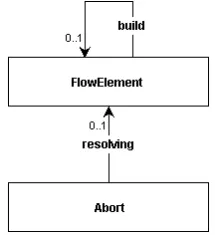
4.1.5 Flow graph construction auxiliaries meta-model

We have two elements that are not present in a completed flow graph, but that we need during its construction: thebuildedge, used for regulating the top-down construction order, and theresolvingedge, introduced for abrupt completion resolution. Figure 4.3 shows the type-graph for these temporary edges.

AFlowElementcan have at most onebuildself-edge, but can have any number of incoming resolvingedges. The source of aresolvingedge always is anAbort.

(34)

4.1.6 Auxiliary production rules for flow graph construction

This section presents several auxiliary rules for flow graph construction that are not specific to a particular programming language, but can be used in flow graph construction systems of any (supported) language.

We have already explained the purpose of the construction rule that introducesentryand exitedges and their initial targets, theFlowConnectors (Figure 4.4).

Figure 4.4: Rule for adding entries and exits to all flow elements.

For conditional branching flow, we often specify that a branch is followed if some condi-tion evaluates totrueorfalse. We assume primitive values to be implicitly present in a flow graph, but due to the fact that thetool [14] does not (yet) support this, they have to be created explicitly by a graph production rule (which is not shown here).

The top-down flow graph construction process has to start at the root-node of a flow graph under construction (for example a MethodBodyin Java). The rule in Figure 4.5 initi-ates the construction process by introducing abuild edge to the root-node (which we label ContextNode). This rule has the highest application priority.

Figure 4.5: Flow graph construction rule for initiating the top-down flow graph construction.

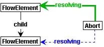
Our abrupt completion resolution process operates bottom-up by propagating the resolv-ingedge from child to parent nodes. Figure 4.6 shows the construction rule that propagates this edge. This rule has the lowest application priority (see Chapter 2), to enable abrupt completion resolution rules to (possibly) match before the propagation is resumed.

(35)

4.2 Flow graph construction rules for Java

As an example of our flow graph meta-model and our approach for designing flow graph construction rules, we have worked out a significant portion of the statements that feature the Java programming language [19].

The statements we have considered are method bodies, blocks of statements, thewhile_, doandforloop statements, the ifandswitchstatement, assignments and several types of expressions, the abrupt completion statementsbreak, continue, return, throw and thetry,

catch_,finally_{exception handling statements.}

For this we have used an abstract graph representation of a partialJava grammar. In Appendix A, this adapted grammar is given. The changes we made to the original Java grammar in the language specification [6] are described in Section 3.1.

In the following sections we present the flow graph construction rules for Java. All construction rules presented below were actually generated by our flow graph meta-rules, which are treated in Chapter 6, from the control flow specifications for Java we will present in Section 5.2.

4.2.1 Method bodies

Method declarations in Java (see [6]) consist of a method signature and a method body. A method body consist of a block of ordered statements. After execution of the method body, control is transferred back to the calling statement (i.e. a method invocation) of the method. TheMethodBodynode is thestartandendpoint of the flow of control in our flow graphs. For eachMethodBodyin an, a flow graph is constructed. TheMethodBodynode is the start point of the top-down flow graph construction process.

The flow graph construction rule of theMethodBody(Figure 4.7) introduces abuildedge to the method’s body. From thereon, thisbuildedge is passed on to sub statements. Theentryof theMethodBodyis merged with theentryof the bodyBlockand thisBlockshares itsexitwith theMethodBody. Thisexitis the end point in the flow graph.

When merging aFlowConnectorwith aFlowElementthe edges of theFlowConnectornode (i.e. its labelFlowConnector, itsentryand itsexit) should be removed (or end up being self-edges of theFlowElement, see Chapter 2). All rules that mergeFlowConnectors feature this eraser edge.

Note that although theBlockin this rule has twoentryedges, these edges will be matched onto the single entry edge of the Block in a flow graph under construction, because the matching can be non-injective.

4.2.2 Blocks of statements

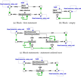
Like most programming languages, Java features sequentially ordered blocks of statements (see [6] p. 361). These statements are executed in order first to last. For convenience, we repeat the relevantrules from our Java grammar in Appendix A.

Block ::= BlockFull | BlockEmpty

BlockFull ::= <LCUR> orderFirst:BlockStatements <RCUR> BlockEmpty ::= <LCUR> <RCUR>

(36)

Figure 4.7: Flow graph construction rule for method-bodies.

BlockStatementsNext ::= Statement orderNext:BlockStatements BlockStatementLast ::= Statement

Ordered lists of statements are handled by four rules (Figure 4.8). The statement ordered first in a (non-empty) statement block receives abuild edge from the block (Figure 4.8(a)). The entry of the block is defined as the entry of the first statement in the block, and the exit of the statements in a block is defined as the exit of the block.

Figure 4.8(b) shows the rule for a block of statements that is empty, i.e. it does not contain sub statements. If this is the case, the block is simply skipped (recall Figure 4.2(c)).

A block can contain any number of statements. The recursive rule is represented in the abstract syntax as a number ofBlockStatements nodes. A BlockStatementsnode has a Statement child, the actual statement, and either anotherBlockStatements node (if it is a BlockStatementsNext), or none (BlockStatementsLast).

We propagate the flow graph construction indicator (thebuildedge) among these Block-Statements, by matching the ordering of statements represented by theorderNextedge (Figure 4.8(c)).

From the exit of the statement we transfer control to the next statement by introducing a flowedge to the entry of theBlockStatementsordered next, which will be the nextStatement, due to the merging of the entry of theBlockStatementsnode with the entry of theStatement node.

In both theBlockStatementsNextRule and the BlockStatementsLastRule(Figure 4.8(d)) we merge the exit of the child statement orBlockStatementsnode with the parentBlockStatements node. The exit of the statement ordered last will therefore be the same node as the exit of the Block.

4.2.3 Conditional statements

Java features two types of conditional statements: theifand theswitch. The if-statement introduces two branches on the value of a Boolean condition, the switch-statement can have any number of branches on the value of a condition of typechar,short,int,byteor anenum

type.

If-statement

(37)

(a) Block - first statement (b) Block - empty

(c) Block-statements - statement ordered next

(d) Block-statements - statement ordered last

Figure 4.8: Flow graph construction rules for blocks of statements.

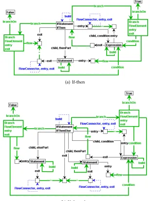
and an optional else-part, which is executed when the condition evaluates tofalse. If the if-statement lacks a then-part, and the condition does not hold, the if-statement is finished.

Figure 4.9(a) shows the flow graph construction rule for an if-statement without an else-part. As one would expect, the rule introduces twoBranches: one branch, taken when the condition evaluates totrue_{, leads to the then-part}Statement. The other leads to the exit of the if-statement, and is taken when the condition does not hold.

Figure 4.9(b) shows the rule for an if-statement with an else-part, which is executed when the condition does not hold.

After execution of thethenPartor theelsePartof an if-statement, the control flow leads to the exit of the if-statement.

Switch-statement

(38)

(a) If-then

(b) If-then-else

Figure 4.9: Flow graph construction rules for if-statement with or without else-part.

Java, this means that after execution of the statements associated with one case, the statements of the case ordered next will be executed. A switch-statement can be terminated prematurely by a break-statement (typically used to prevent this fall-through).

The production rules of the switch-statement are shown in Figure 4.11. Both the Switch-Block and theSwitchBlockStatementGroupsnodes are containers in the syntax representation that have no actual control flow semantics.

(39)

The production rule in Figure 4.2.3 shows that upon entering a switch-statement, the expression is first executed, next the flow is transferred to theSwitchStatementnode.

The branching behavior of the switch-statement is represented by aBranchfor every case label present. The rule in Figure 4.12(a) adds a branch from theSwitchStatement decision node, on theSwitchLabel’s value, to the entry of theStatementassociated with the case label. As can be concluded when considering our flow graph meta-model (Figure 3.5), we have a special representation for thedefaultcase (Figure 4.12(b)).

Figure 4.10: Flow graph construction rule for the switch-statement.

4.2.4 Loop statements

Java features three kinds of loop-statements: thewhile_,do_andfor_{. The while-statement and}

do-statement are minor variations of eachother. The for-statement has eight variations, all having their own control flow semantics.

While-statement

The while-statement in Java (see [6] p. 380) executes a statement (the body) repeatedly as long as the loop condition holds. The body can ofcourse be a block of statements. The loop condition is a boolean expression.

Control flow enters the while-statement (Figure 4.13) at the loop conditionExpression. At theWhileStatementnode, a decision is made. OneBranchenters thebodyof the while-statement and the other proceeds directly to theexitof the while-statement. The former branch is taken when the loop-condition evaluates totrue_{and the latter branch is taken when the condition}

evaluates tofalse. After execution of the bodyStatement, the loop conditionExpressionis evaluated again (i.e. aflowedge is introduced from theexitof theStatementto theentryof the Expression).

Do-statement

(40)

(a) Switch-block

(b) Switch-block-statement-groups - ordered next

(c) Switch-block-statement-groups - ordered last

(d) Switch-block-statement-group

Figure 4.11: Flow graph construction rules for switch-block-statements-groups.

For-statement

(41)

(a) Switch-label (b) Switch-label - default

Figure 4.12: Flow graph construction rules for switch-labels.

Figure 4.13: Flow graph construction rule for while-statements.

1. ForEver: for-statement without init-, condition- or update-part (Figure 4.15);

2. ForWithInit: for-statement with init-part only (not shown);

3. ForWithInitCondition: for-statement with init- and condition-part (not shown);

4. ForWithInitConditionUpdate: for-statement with init-, condition- and update-part (Figure 4.16);

5. ForWithInitUpdate: for-statement with init- and update-part (not shown);

6. ForWithCondition: for-statement with condition-part only (not shown);

(42)

Figure 4.14: Flow graph construction rule for do-statements.

8. ForWithUpdate: for-statement with update-part only (Figure 4.17).

The init-part of a for-statement performs initialization of the loop counter(s). The condition-part is the loop-condition and equivalent to the condition in the while-statement and do-statement. The update-part updates the loop counter(s) after each iteration of the body of the for-statement.

TheForEvervariant (Figure 4.15) iterates its body continuously, i.e. forever. This is very similar to a while-statement that features the Boolean literaltrueas loop condition, although in the case of awhile(true)the literal expression is evaluated each iteration and theBranch ontrue_{is followed each iteration.}

Figure 4.15: Flow graph construction rule for the for-statement without init-, condition- or update-part.

The ForWithInitvariant (rule omitted here)performs some initialization of loop counters and then starts to iterate its body continuously, i.e. forever.

The ForWithInitCondition variant (rule omitted here)performs some initialization of loop counters, evaluates its loop condition and executes its body if its condition evaluated totrue_.

Like the while-statement, the expression is evaluated again after each iteration of the body to decide whether to iterate the body again.