Knots, Trees, and Fields: Common Ground Between Physics and Mathematics

(1)

common ground between physics and mathematics

Thesis by

Ingmar Akira Saberi

in partial fulfillment of the requirements for the degree of

Doctor of Philosophy in Physics

CALIFORNIA INSTITUTE OF TECHNOLOGY Pasadena, California

2017

(2)

(3)

(4)

ACKNOWLEDGEMENTS

This thesis represents the culmination of a five-year sojourn at Caltech. During that time, and throughout my life, I have been incomparably fortunate to have the love, kindness, generosity, and support of many wonderful people. Nothing would have been possible without you all. As much as I hope I will mention each of you here, I am quite confident I will fail; this reflects no lack of gratitude on my part, but only an (unfortunately characteristic) lack of due diligence. First and foremost, I owe a profound debt to my advisor, Sergei Gukov. I learned a tremendous amount from him, and his steadfast support throughout my time in graduate school allowed me to learn and accomplish as much as I have. Sergei, I am enormously lucky and grateful to have had the chance to be your student.

In addition, I would like to thank from the bottom of my heart the other people I have had the pleasure of collaborating with on the work that makes up this thesis: Matt Heydeman, Hyungrok Kim, Matilde Marcolli, Satoshi Nawata, Bogdan Stoica, Marko Stoˇsi´c, and Piotr Su lkowski. Each of you was a valued teacher and coworker, and I quite simply could not have done it without you. Many, many thanks.

Matilde deserves particular mention for her service on my committee. I am profoundly grateful to her, and to the committee’s other members, Maria Spi-ropulu and John Schwarz, for support, friendship, and advice, and for stead-fastly standing in my corner. Also, Maria, special thanks to you and also to Sarah Reisman: it has been a pleasure to have undeservedly been a part of so many of both your respective groups’ activities.

(5)

and Bureau of Land Management—its public lands and wilderness preserves in perpetuity (and, as such, for my own and everyone else’s sanity). I must also gratefully acknowledge the Walter Burke Institute for Theoretical Physics at Caltech, of which I have been a part since its inception a few years ago, for its stimulating research environment; thanks are due to all its faculty, and in particular to D. Politzer for support and for many invaluable stories. Also, no mention of the Burke Institute would be complete without an appreciative nod to Carol Silberstein, without whose tireless efforts everything would have come apart at the seams long ago.

(6)

I owe special mention to my long-time office mate (and more recent roommate), T. McKinney, from whom I learned an enormous amount about physics and even more about the Abrahamic concept of land ownership, rituals of perfor-mative alterity among the Hopi, and a panoply of other topics. Thanks to you for putting up with me so frequently, as well as to all other aficionados of card-playing and pretentious movies: A. Arjun, B. Pang, K. Cha lupka (m´oj przyjaciel), L. Sun, and the new arrival (mazel tov!).

Thanks to LKV for being an old friend and familiar face in L.A., to N. Ka-dunce and J. Hammond for becoming (albeit by a slim margin) my first new friends here and for five years of stalwart companionship and good food, to A. Jackson for getting me back into the garden, tomi primoErnie for five years of lunches, to YGB for dependability and brotherhood (don’t be as much of a stranger next time!), to NAD for (co?)-originating “Handles; Messiah,” and to bandmates and travel companions C. Pe˜na and C. Fernandez (congratulations to you both!).

To the close friends, companions, and roommates I have been lucky to count as family by any other name: thank you for everything over the last five years. JMGD and KLJ, good luck to you both in Chicago; the Midwest just got a little more young and restless. EAQ, EGG (couldn’t resist), and Sofia Celeste, I aspire to have a family as beautiful as yours.

Onward. Love and gratitude to the happy couple, JCL and YDN—eagerly looking forward to celebrating with you on Labor Day; to LPM, for the countless ways in which you have enriched and continue to enrich my life— congratulations on hitting the big time; to BDW for being a human being of the very first water and for literally thousands of dollars’ worth of accommo-dation, for which I promise I will someday find a way to repay you; to BEK for being a first-rate mathematician, for commiseration, and for continuing to costar in “Separated at Birth;” to ORK for going to buy stamps with me on that fateful day in 2007; and finally to DCG, for bringing great joy into my life these past months.

(7)

ABSTRACT

One main theme of this thesis is a connection between mathematical physics (in particular, the three-dimensional topological quantum field theory known as Chern-Simons theory) and three-dimensional topology. This connection arises because the partition function of Chern-Simons theory provides an invariant of three-manifolds, and the Wilson-loop observables in the theory define invari-ants of knots. In the first chapter, we review this connection, as well as more recent work that studies the classical limit of quantum Chern-Simons theory, leading to relations to another knot invariant known as the A-polynomial. (Roughly speaking, this invariant can be thought of as the moduli space of flat SL(2,_C) connections on the knot complement.) In fact, the connection can be deepened: through an embedding into string theory, categorifications of polynomial knot invariants can be understood as spaces of BPS states. We go on to study these homological knot invariants, and interpret spectral sequences that relate them to one another in terms of perturbations of super-symmetric theories. Our point is more general than the application to knots; in general, when one perturbs any modulus of a supersymmetric theory and breaks a symmetry, one should expect a spectral sequence to relate the BPS states of the unperturbed and perturbed theories. We consider several diverse instances of this general lesson. In another chapter, we consider connections between supersymmetric quantum mechanics and the de Rham version of ho-motopy theory developed by Sullivan; this leads to a new interpretation of Sullivan’s minimal models, and of Massey products as vacuum states which are entangled between different degrees of freedom in these models.

We then turn to consider a discrete model of holography: a Gaussian lattice model defined on an infinite tree of uniform valence. Despite being discrete, the matching of bulk isometries and boundary conformal symmetries takes place as usual; the relevant group is PGL(2,_Qp), and all of the formulas developed for holography in the context of scalar fields on fixed backgrounds have natural analogues in this setting. The key observation underlying this generalization is that the geometry underlying AdS3/CFT2 can be understood algebraically,

(8)

PUBLISHED CONTENT AND CONTRIBUTIONS

Much of this thesis is adapted from articles that originally appeared in other forms. All are available as arXiv preprints; where appropriate, the DOI for the published version is included as a hyperlink from the journal citation. (Should the reader wish, hovering the mouse over the link will reveal the explicit DOI.) [3] (adapted for chapter1) is a review article, based on summer-school lectures given by my advisor; I was responsible for exposition and for preparing the manuscript from rough lecture notes. The remaining chapters are original re-search articles: [5] appears as chapter2and [4] as chapter4, while chapter3is adapted from those sections of [1] from which I was most intimately involved. Chapter 5 consists of the draft of an unpublished article detailing another re-search project I undertook in graduate school. All authors contributed equally to [4] and [5]; I was largely responsible for the content of [2].

1_{S. Gukov, S. Nawata, I. Saberi, M. Stoˇsi´}_{c, and P. Su lkowski. “Sequencing}

BPS spectra.” JHEP03, 004. (2016). arXiv:1512.07883 [hep-th].

2_{S. Gukov and I. Saberi. “Motivic quantum field theory and the number}

theory of A-polynomial curves.” To appear.

3_{S. Gukov and I. Saberi. “Lectures on knot homology and quantum curves.”}

In Topology and field theories. Edited by S. Stolz. Contemporary Math-ematics 613. (American Mathematical Society. 2014). arXiv:1211 . 6075 [hep-th].

4_{M. Heydeman, M. Marcolli, I. Saberi, and B. Stoica. “Tensor networks,} p-adic fields, and algebraic curves: arithmetic and the AdS3/CFT2

corre-spondence.” (2016).arXiv:1605.07639 [hep-th].

5_{H. Kim and I. Saberi. “Real homotopy theory and supersymmetric quantum}

(9)

LIST OF FIGURES

Number Page

1.1 The three Reidemeister moves . . . 10

1.2 The trefoil knot . . . 14

1.3 The knots 51 and 10132 . . . 16

1.4 Mutant knots . . . 19

1.5 The torus T2 =∂N(K) for K = unknot, with cycles m and `. . 21

1.6 The simple harmonic oscillator . . . 28

1.7 The setup for Chern-Simons theory . . . 33

1.8 The Khovanov homology Hi,j(K = 31) of the trefoil knot. . . . 43

1.9 The HOMFLY homology for knots 51 and 10132 . . . 46

1.10 Relations between homological and polynomial invariants . . . 46

2.1 The de Rham complex of a compact manifold . . . 56

2.2 The Borromean rings . . . 59

2.3 The Hodge diamond of a connected K¨ahler threefold . . . 70

2.4 The action of the B2 root system on the Hodge diamond of a hyper-K¨ahler manifold. . . 73

2.5 Some weight diagrams for representations of SO(5) . . . 75

2.6 A non-formal example of a minimal-model CDGA . . . 80

2.7 A subgroup diagram for R-symmetries of various theories . . . 87

2.8 Illustration of the differences between requirements tabulated in Fig. 2.7. . . 89

2.9 Hodge diamonds of compact hyper-K¨ahler eight-manifolds . . . 90

3.1 The moduli space of scalar supercharges . . . 105

3.2 A “staircase” representation in a bicomplex . . . 109

3.3 Single letters in a chiral multiplet annihilated by Q−. . . 111

3.4 Superpotential deformations of the chiral ring . . . 115

3.5 Single letters in a vector multiplet annihilated by Q₋. . . 116

3.6 Single letters contributing to the index . . . 120

3.7 Various limits of the N = 2 index . . . 121

3.8 A Landau-Ginzburg model on a strip . . . 123

(12)

3.10 Fusion of topological defects . . . 135

3.11 Defects in Landau-Ginzburg theory on a cylinder . . . 136

3.12 The Landau-Ginzburg model for the unknot . . . 138

3.13 Dimensional reduction of the fivebrane system . . . 140

3.14 Unreduced sl(2) homology of the trefoil . . . 143

3.15 Vacuum degeneracies lifted by perturbation . . . 145

4.1 The Bruhat–Tits tree . . . 153

4.2 Loxodromic symmetries of the Bruhat–Tits tree . . . 157

4.3 The Euclidean BTZ black hole . . . 161

4.4 Fundamental domains for the action of Γ on H3. . . 162

4.5 Uniform spanning trees of uniform tilings . . . 174

4.6 Constructing uniform spanning trees . . . 176

4.7 Tiling the periphery of a causal wedge . . . 179

4.8 The p-adic integers _Zp . . . 195

4.9 Open sets in P1₍ Qp) . . . 201

4.10 The p-adic BTZ black hole . . . 207

4.11 Drinfeld’s p-adic upper half plane and the Bruhat–Tits tree. . 209

4.12 Translation along a tree geodesic . . . 210

5.1 The data of a physical theory . . . 217

5.2 Real slices of A-polynomials . . . 230

(13)

I will take an egg out of the robin’s nest in the orchard,

I will take a branch of gooseberries from the old bush in the garden, and go and preach to the world;

You shall see I will not meet a single heretic or scorner, You shall see how I stump clergymen, and confound them,

You shall see me showing a scarlet tomato, and a white pebble from the beach.

(14)

INTRODUCTION

This thesis consists of work that was originally published during my graduate-school career in the form of a series of distinct papers [109, 111, 119, 133], as well as a small amount of material from work that has yet to appear [110]. As such, the various chapters range across several different and seemingly distant topics; nonetheless, I feel that certain key themes underlie and unify all of it. Chief among these themes is the idea of bridging the gap between the disciplines now termed theoretical physics and pure mathematics.

Historically speaking, no distinction was generally made between these two disciplines until the twentieth century. As the pace of scientific discovery and concomitant specialization accelerated—and, in particular, as the project of quantum field theory came to bear fruit, requiring physicists to accept tech-niques such as renormalization whose basis in rigorous mathematics was ob-scure at best—the gulf between the two grew to appear nearly insurmountable. In 1972, Freeman Dyson quipped in his Gibbs memorial lecture that, “[as] a working physicist, I am acutely aware of the fact that the marriage between mathematics and physics, which was so enormously fruitful in past centuries, has recently ended in divorce” [73]. Dyson’s classic lecture goes on to de-scribe various instances in the history of science when the division between these two fields impoverished both. In many cases, a subject of interest to one group would have been advanced considerably by an influx of the ideas or the expertise of the other; the advances in question were uncovered years—and sometimes many years—later than they might have been. In closing, he rec-ommended a selection of problems from quantum field theory and quantum gravity to the attention of pure mathematicians.

Dyson was prophetic. The renewal of the dialogue between these two disci-plines began in earnest not long afterwards. While there are many stones at which one might point to mark the initial moment, C. N. Yang’s 1977 pa-per [223], which pointed out the intimate connection between the physics of gauge theories and the theory of fiber bundles studied in mathematics, seems as good as any (at least from the viewpoint of someone who was not yet born at the time).

(15)

Donaldson’s landmark 1983 paper [70] used ideas from gauge theory to con-struct a powerful new invariant of smooth con-structures on four-manifolds. The key idea of his work is simple enough to describe: One studies the smooth space X by first producing a certain auxiliary space, M(X), which is the moduli space of solutions to certain partial differential equations (the anti-self-dual instanton equations) on X. The topology of this moduli space depends sensitively on the smoothness structure with respect to which the PDEs are defined; relatively crude topological invariants of M(X), such as its homol-ogy, then become sophisticated and subtle invariants of X as a smooth space. (Other papers from around the same time [5, 27] also evidence the renewed mutual interest among members of both camps.)

Gauge theory soon made other related appearances in mathematics. Several years later, using similar PDEs, Andreas Floer [80–82] defined the homol-ogy theories for three-manifolds and Lagrangian intersections that bear his name. It was noticed that the generalizations of Donaldson’s invariants to a four-manifold X with boundary ∂X = Y were naturally valued in the Floer homology groups of Y. In 1988, Edward Witten was able to interpret these constructions from a physical perspective, showing that Donaldson’s invariants were naturally computed by a particular truncation of a supersymmetric Yang-Mills theory. Almost simultaneously, Sir Michael Atiyah [7,8] gave axioms for the general notion of a topological quantum field theory.

Topological field theory, or TQFT, is a fitting synecdoche for the interdisci-plinary field that has continued to grow out of these early papers. TQFTs are of interest to physicists as toy models that possess many of the essential features of quantum field theory—or as truncated sectors of field theories of physical interest—while remaining simple enough to be mathematically rig-orous and exactly solvable. Mathematicians usually think of TQFT as an organizing principle for existing invariants of manifolds, or a source of new invariants. As evidenced by Donaldson’s theory, attempting to classify geo-metric spaces using the data of how physical theories behave on those spaces has proved enormously fruitful.

(16)

are given by d-manifolds X with boundary ¯Y0 tY1 (where the bar denotes

orientation reversal). Put succinctly, the morphisms are oriented cobordisms. One is to imagine that, as in a usual physical theory, the state of the system is specified on a codimension-one surface playing the role of a constant-time slice, and the cobordism plays the role of a generalized time-evolution during which topology change is possible.

As is usual in quantum mechanics, the data of the theory consists of kinematic data (a description of its possible states) together with dynamical data (how those states evolve in time). The collection of possible states of the system on a space Yi forms a Hilbert space, which we will denote Hi. Time evolution provides a mapping of states, so that we should be able to associate to each cobordism X a mapping φX : H0 → H1. There are additional requirements

and possible variants of these axioms, but the essential structure is hopefully clear.

In more mathematical language, one says that a TQFT is a symmetric mon-oidal functor from a geometric category (the cobordism category Cob(d) de-scribed in the previous paragraphs) to the linear category Vect. “Symmetric monoidal” just means that the functor should preserve tensor products: it carries the disjoint union of manifolds and cobordisms between them to the usual tensor product of Hilbert spaces and linear maps. In the special case where the d-manifold X has empty boundary, one gets a morphism between empty (d₋1)-manifolds; this amounts to a linear map between copies of _C, which is a numerical invariant.

TQFTs fit into the general theme in mathematics of studying complicated, abstract, or geometric objects, such as groups, by considering their linear rep-resentations. Suppose that one were to consider an ordinary group G, viewed as a category with one object and only invertible morphisms. One could then ask for a functor from this category toVect. This would amount to a choice of vector space V, to be associated to the object, and a homomorphism from G

(which is the automorphisms of the unique object in the source category) to the linear automorphism group of V. In other words, one recovers the usual notion of a linear representation on an arbitrary vector space! It is easy to see from this description that a TQFT generalizes the notion of linear represen-tation to a rather different and more complicated source category.

(17)

defined by topological field theories, in the form of surprising and unexpected conjectures. This is possible because the physical understanding of such an invariant is rarely as an isolated construction. Rather, the TQFT describes one piece of, or calculation in, a much larger and more baroque structure: a quantum field theory. If one believes that the quantum field theory makes sense, and can see how a mathematical object fits in as a piece of it, then one has many new angles from which to look at that object, and many new relations to expect between it and other pieces of the QFT.

One interesting example of an advance that was made using this kind of rea-soning took place in 1994, when Seiberg and Witten [183, 184] analyzed the infrared behavior of theN = 2 supersymmetric SU(2) Yang-Mills theory that Witten had previously related to Donaldson’s invariants. Using standard phys-ical techniques, they argued that the theory should undergo a phase transition to a symmetry-breaking phase at low energy scales, in which the nonabelian interactions of the SU(2) theory should be replaced by an effective descrip-tion in terms of abelian U(1) gauge theory. One can think of this transidescrip-tion as analogous to electroweak symmetry breaking in the Standard Model of particle physics. However, Witten had previously argued that the twist of this theory that produced Donaldson’s invariants was independent of scale; it followed that the invariants should be able to be computed using the simpler effective physics in the infrared [214]. For mathematicians, the end result was a new set of seemingly unrelated partial differential equations (the Seiberg–Witten equations), which were far easier to deal with than Donaldson’s equations, but which could be used in similar fashion to compute invariants carrying nearly identical information.

(18)

to classical Chern-Simons theory, which is called the A-polynomial. The zero locus of this polynomial is the moduli space of solutions to the equations of motion in SL(2,_C) Chern-Simons theory. He further observed that quantiza-tion should associate to this space a recurrence relaquantiza-tion (the analogue of the Schr¨odinger equation), whose solution is the set of “colored” Jones polyno-mials associated to arbitrary representations of G = SU(2). This prediction (now verified in special cases and checked in many examples) is known as the

AJ-conjecture.

In Chapter 1, taken from the work [111] by Gukov and myself, we give a pedagogical review of these developments, discussing the connections between knot theory and knot invariants, topological field theory, and quantization. We also treat newer developments in the subject, related to categorified quantum group invariants—i.e., knot homologies. From the perspective of physics, knot homologies can be understood as spaces of BPS states in certain theories that can be geometrically engineered from M-theory, taking the data of the knot as an input. (This interpretation is reviewed later in the thesis, in §3.2.) Chapter 2, written with Hyungrok Kim [133], explores the theme of using the states or operators of a physical theory defined on a geometric space as an algebraic model of that space. We focus on the simplest possible exam-ple, supersymmetric quantum mechanics, pointing out that the approach to homotopy theory over a field pioneered by Sullivan [190] is closely connected to physics, and giving a new interpretation of Massey products in topology as vacuum states in certain quantum-mechanical models (Sullivan’s minimal models) that are entangled between different degrees of freedom.

(19)

broader and has nothing to do with knotsper se.

In Chapter4, based on [119] and written with Heydeman, Marcolli, and Stoica, the same theme is expressed in a much different context. We were interested in the question of how best to construct models of holography in which space-time is discrete. This has been of interest recently in light of speculation that tensor-network models, which reproduce certain features of conformal field theory such as the entanglement entropy of the ground state, can be under-stood as discrete analogues of hyperbolic bulk geometry. Our models appeal to a different angle of generalization, inspired by previous work of Manin and Marcolli: we formulate AdS3/CFT2 as algebraically as possible, and then

con-sider changing the underlying field in the construction of the spacetime to be a p-adic field rather than _C. The resulting bulk geometry is a p-adic maxi-mally symmetric space: the Bruhat–Tits tree of SL(2,_Qp). While this space is naturally discrete, it does not break any symmetries; one can still make sense of both bulk isometries and boundary conformal transformations, and identify the two as is required for the normal holographic dictionary to work.

We demonstrate that, at least for massive free scalar fields in a fixed back-ground geometry, the holographic dictionary can be developed exactly as in the ordinary case. Certain features of AdS/CFT, such as the correspondence between the holographic direction and the boundary RG scale, are present even more sharply in our models than in the ordinary case. We also give arguments that logarithmic scaling of the entanglement entropy should hold; given this, an analogue of the Ryu-Takayanagi formula follows trivially from the geometry of the tree. Based on this, we argue that thep-adic geometry (rather than the archimedean geometry) is the natural setting in which to make contact with tensor network models, and we offer some examples of constructions through which this might be done.

(20)

Chapter 1

QUANTIZATION AND CATEGORIFICATION IN

TOPOLOGICAL QUANTUM FIELD THEORY

1_{S. Gukov and I. Saberi. “Lectures on knot homology and quantum curves.”}

In Topology and field theories. Edited by S. Stolz. Contemporary Math-ematics 613. (American Mathematical Society. 2014). arXiv:1211 . 6075 [hep-th].

Foreword

The lectures in this chapter will by no means serve as a complete introduction to the two topics of quantizationand categorification. These words represent not so much single ideas as broad tools, programs, or themes in physics and mathematics; both are areas of active research, and are still not fully under-stood. One could easily give a full one-year course on each topic separately. Rather, the goal of these lectures is to serve as an appetizer: to give a glimpse of the ideas behind quantization and categorification, by focusing on very concrete examples and giving a working knowledge of how these ideas are manifested in simple cases. It is our hope that the resulting discussion will remain accessible and clear while shedding at least some light on these complex ideas, and that the interest of the reader will be piqued.

Imagine the category of finite-dimensional vector spaces and linear maps. To each object in this category is naturally associated a number, the dimension of that vector space. Replacing some collection of vector spaces with a collection of numbers in this way can be thought of as a decategorification: by remem-bering only the dimension of each space, we keep some information, but lose all knowledge about (for instance) morphisms between spaces. In this sense, decategorification forgets about geometry.

(21)

in the affirmative to this question is a categorification of that invariant. Perhaps the most familiar example of categorification at work is the reinterpre-tation of the Euler characteristic as the alternating sum of ranks of homology groups,

χ(M) =X k≥0

(₋1)krankHk(M). (1.1)

In light of this formula, the homology of a manifold M can be seen as a categorification of its Euler characteristic: a more sophisticated and richly structured bearer of information, from which the Euler characteristic can be distilled in some natural way. Moreover, homology theories are a far more powerful tool than the Euler characteristic alone for the study and classification of manifolds and topological spaces. This shows that categorification can be of practical interest: by trying to categorify invariants, we can hope to construct stronger invariants.

(22)

topol-ogy, which indeed is often called “quantum” topology. This is the arena in which we will study the implications of quantization and categorification, pri-marily for the reason that it allows for many concrete and explicit examples and computations. Specifically, almost all of our discussion will take place in the context of knot theory. The reader should not, however, be deceived into thinking of our aims as those of knot theorists! We do not discuss quantization and categorification for the sake of their applications to knot theory; rather, we discuss knot theory because it provides a window through which we can try and understand quantization and categorification.

1.1 Why knot homology?

A knot is a smooth embedding of a circleS1 as a submanifold of S3:

k:S1 ,_→S3, K = imˆ k. (1.2) See e.g.Figs.1.2 and1.3 for some simple examples. Likewise, alink is defined as an embedding of several copies of S1_{. Two knots are equivalent if the two}

embeddings k and k0 can be smoothly deformed into one another through a family of embeddings, i.e., without self-intersections at any time. One should think of moving the knot around in the ambient space without breaking the string of which it is made.

In studying a knot, one usually depicts it using a planar knot diagram: this should be thought of as a projection of the knot from _R3 ₌ _S3 _{\ {}_pt._}_{, in}

which it lives, to some plane _R2 _⊂

R3. Thus, a knot diagram is the image of an immersion of S1 _in

R2, having only double points as singularities, and with extra data indicating which strand passes over and which under at each crossing. Examples of knot diagrams can be seen in Figs.1.2, 1.3, and 1.4. It should be clear that there is no unique diagram representing a given knot. We could obtain very different-looking pictures, depending on the exact em-bedding in _R3 _{and on the choice of plane to which we project. Two knot}

(23)

R1: _⇔ _⇔

R2: _⇔ R3: _⇔

Figure 1.1: The three Reidemeister moves, which generate all equivalences between knot diagrams.

show replacements that can be made in any portion of a knot diagram to give an equivalent diagram.

Finding a sequence of Reidemeister moves that changes one given knot diagram into another, or showing that no such sequence exists, is still an ad hoc and usually intractable problem. As such, in attempting to classify knots, more clever methods are important. One of the most basic tools in this trade is a knot invariant: some mathematical object that can be associated to a knot, that is always identical for equivalent knots. In this way, one can definitively say that two knots are distinct if they possess different invariants. The con-verse, however, is not true; certain invariants may fail to distinguish between knots that are in fact different. Therefore, the arsenal of a knot theorist should contain a good supply of different invariants. Moreover, one would like invari-ants to be as “powerful” as possible; this just means that they should capture nontrivial information about the knot. Obviously, assigning the number 0 to every knot gives an invariant, albeit an extremely poor one!

Since one usually confronts a knot in the form of one of its representative knot diagrams, it is often desirable to have an invariant that can be efficiently computed from a knot diagram. Showing that some such quantity associated to a diagram is actually an invariant of knots requires demonstrating that it takes the same values on all equivalent diagrams representing the same knot. Reidemeister’s theorem makes this easy to check: to show that we have defined a knot invariant, we need only check its invariance under the three moves in Fig. 1.1.∗

(24)

Given the goal of constructing knot invariants, it may be possible to do so most easily by including some extra structure to be used in the construction. That is, one can imagine starting not simply with a knot, but with a knot “decorated” with additional information: for instance, a choice of a Lie algebrag= Lie(G) and a representation R ofg. It turns out that this additional input data from representation theory does in fact allow one to construct various invariants (numbers, vector spaces, and so on), collectively referred to asquantum group invariants. A large part of these lectures will consist, in essence, of a highly unorthodox introduction to these quantum group invariants.

The unorthodoxy of our approach is illustrated by the fact that we fail com-pletely to address a natural question: what on earth do (for instance) the quantum sl(N) invariants have to do with sl(N)? Representation theory is almost entirely absent from our discussion; we opt instead to look at an alter-native description of the invariants, using a concrete combinatorial definition in terms of so-called skein relations. A more full and traditional introduction to the subject would include much more group theory, and show the construc-tion of the quantum group invariants in a way that makes the role of the additional input datagand Rapparent [175,212]. That construction involves assigning a so-called “quantum R-matrix” to each crossing in a knot diagram in some manner, and then taking a trace around the knot in the direction of its orientation. The connection to representation theory is made manifest; the resulting invariants, however, are the same.

Example 1. Suppose that we take an oriented knot together with the Lie

algebra g = sl(N) and its fundamental N-dimensional representation. With this special choice of extra data, one constructs the quantum sl(N) invariant, denoted PN(K;q). Although it makes the connection to representation theory totally obscure, one can compute PN(K;q) directly from the knot diagram using the following skein relation:

qNPN(

?

_

)₋q−NPN(

?

_

) = (q₋q−1)PN(

o

o //

). (1.3)

(25)

For now, one can think of q as a formal variable. The subdiagrams shown in (1.3) should be thought of as depicting a neighborhood of one particular crossing in a planar diagram of an oriented knot; to apply the relation, one replaces the chosen crossing with each of the three shown partial diagrams, leaving the rest of the diagram unchanged.

To apply this linear relation, one also needs to fix a normalization, which can be done by specifyingPN for the unknot. Here, unfortunately, several natural choices exist. For now, we will choose

PN( ) =

qN ₋q−N q₋q−1 =q

−(N−1)₊_q−(N−3)₊

· · ·+qN−1

| {z }

Nterms

. (1.4)

This choice gives the so-called unnormalized sl(N) polynomial. Notice that, given any choice of PN( ) with integer coefficients, the form of the skein relation implies that PN(q)∈Z[q, q−1] for every knot.

Notice further that, with the normalization (1.4), we have

PN( )−−→

q→1 N, (1.5)

which is the dimension of the representation R with which we decorated the knot, the fundamental ofsl(N). We remark that this leads to a natural general-ization of the notion of dimension, the so-called quantum dimension dimq(R) of a representation R, which arises from the quantum group invariant con-structed from R evaluated on the unknot.

Equipped with the above rules, let us now try to compute PN(q) for some simple links. Consider the Hopf link, consisting of two interlocked circles:

o

/

Applying the skein relation to the upper of the two crossings, we obtain:

qNPN

h o o / / Hopf link i

−q−NPN

h o o / / two unknots i

= (q₋q−1)PN

h o o / / one unknot i . (1.6)

(26)

just for knots, since application of the relation (1.3) may produce links with more than one component. This means that the normalization (1.4) is not quite sufficient; we will need to specifyPN onk unlinked copies of the unknot, for k _≥1.

As such, the last of our combinatorial rules for computing PN(q) concerns its behavior under disjoint union:

PN( tK) =PN( )·PN(K), (1.7) where K is any knot or link. Here, the disjoint union should be such that K

and the additional unknot are not linked with one another.

Caution: The discerning reader will notice that our final rule (1.7) is not linear, while the others are, and so is not respected under rescaling of PN(q). Therefore, if a different choice of normalization is made, it will not remain true that PN(k unknots) = [PN( )]k. The nice behavior (1.7) is particular to our choice of normalization (1.4). This can be expressed by saying that, in making a different normalization, one must remember to normalize only one copy of the unknot.

To complete the calculation we began above, let’s specialize to the caseN = 2. Then we have

P2( ) =q−1 +q =_⇒ P2( _/_/ _o_o ) = (q−1+q)2 =q−2+ 2 +q2. (1.8) Applying the skein relation (1.6) then gives

q2P2( // oo ) =q−2(q−2+ 2 +q2) + (q−q−1)(q+q−1)

=q−4+q−2+ 1 +q2,

(1.9)

so that

P2( // oo ) =q−6+q−4+q−2+ 1. (1.10)

We are now ready to compute the sl(N) invariant for any link.

From the form of the rules that define this invariant, it is apparent that de-pendence on the parameter N enters the knot polynomial only by way of the combination of variablesqN. As such, we can define the new variable a=ˆ qN, in terms of which our defining relations become

(27)

Figure 1.2: The trefoil knot 31. (Image from [177].)

Pa,q( ) =

a₋a−1

q₋q−1. (1.12)

Together with the disjoint union property, these rules associate to each ori-ented link K a new invariant Pa,q(K) in the variables a and q, called the (unnormalized) HOMFLY-PT polynomial of the link [88]. This is something of a misnomer, since with the normalization (1.12) the HOMFLY-PT invari-ant will in general be a rational expression rather than a polynomial. We have traded the two variables q, N for q and a.

For various special choices of the variablesa andq, the HOMFLY-PT polyno-mial reduces to other familiar polynopolyno-mial knot invariants:

• a=qN_{, of course, returns the quantum} _sl₍_N_{) invariant} _P N(q).

• With the particular choicea =q2(N = 2), the HOMFLY-PT polynomial becomes the classicalJones polynomial J(L;q)_≡P2(q),

J(K;q) = P_a₌_q2_,q(K). (1.13)

Discovered in 1984 [123], the Jones polynomial is one of the best-known polynomial knot invariants, and can be regarded as the “father” of quan-tum group invariants; it is associated to the Lie algebra sl(2) and its fundamental two-dimensional representation.

(28)

Now, the attentive reader will point out a problem: if we try and compute the Alexander polynomial, we immediately run into the problem that (1.12) requires P1,q( ) = 0. The invariant thus appears to be zero for every link! However, this does not mean that the Alexander polynomial is trivial. Remem-ber that, since the skein relations are linear, we have the freedom to rescale invariants by any multiplicative constant. We have simply made a choice that corresponds, for the particular valuea= 1, to multiplying everything by zero. This motivates the introduction of another convention: the so-called normal-ized HOMFLY-PT polynomial is defined by performing a rescaling such that

Pa,q( ) = 1. (1.14)

This choice is natural on topological grounds, since it associates 1 to the unknot independent of how the additional input data, or “decoration,” is chosen. (By contrast, the unnormalized HOMFLY-PT polynomial assigns the value 1 to the empty knot diagram.) Taking a = 1 in the normalized HOMFLY-PT polynomial returns a nontrivial invariant, the Alexander polynomial.

Exercise 1. Compute the normalized and unnormalized HOMFLY-PT

poly-nomials for the trefoil knot K = 31 (Fig. 1.2). Note that one of these will

actually turn out to be polynomial!

Having done this, specialize to the case a = q2 to obtain the normalized and unnormalized Jones polynomials for the trefoil. Then specialize to the case

a=q. Something nice should occur! Identify what happens and explain why this is the case.

Solution. Applying the skein relation for the HOMFLY-PT polynomial to one crossing of the trefoil knot gives

aPa,q(31)−a−1Pa,q( ) = (q−q−1)Pa,q( // oo ).

Then, applying the relation again to the Hopf link (as in the above example) gives

aPa,q( _/_/ _o_o )₋a−1Pa,q( // oo ) = (q−q−1)Pa,q( ). Therefore, for the unnormalized HOMFLY-PT polynomial,

P(31) =a−2P( ) +a−2(q−q−1)

(29)

Figure 1.3: The knots 51 and 10132. (Images from [177].)

which becomes

P(31) =

a₋a−1 q₋q−1

a−2q2+a−2q−2₋a−4.

The normalized HOMFLY-PT polynomial is simply the quantity in brackets. Specializing to a=q2 _{gives the unnormalized Jones polynomial:}

P2(31) =

q2₋q−2 q₋q−1

q−2+q−6₋q−8. (1.15) Again, the normalized Jones polynomial is the factor in square brackets. Fi-nally, we specialize to a = q, obtaining P = 1 in both the normalized and unnormalized cases! This is connected to the fact that a = q corresponds to constructing the sl(1) invariant, which must be vacuous since the Lie algebra is trivial.

Remark 1. The study of this subject is made more difficult by the

prepon-derance of various conventions in the literature. In particular, there is no agreement at all about standard usage with regard to the variables for poly-nomial invariants. Given ample forewarning, this should not cause too much confusion, but the reader must always be aware of the problem. In particu-lar, it is extremely common for papers to differ from our conventions by the replacement

a _7→a1/2, q _7→q1/2, (1.16) halving all powers that occur in knot polynomials. Some authors also make the change

(30)

We have by now seen a rich supply of knot polynomials, which can be straight-forwardly computed by hand for simple enough diagrams, and are easy to write down and compare. One might then ask about the value of attempting to cate-gorify at all. Given such simple and powerful invariants, why would one bother trying to replace them with much more complicated ones?

The simple answer is that the HOMFLY-PT polynomial and its relatives, while powerful, are not fully adequate for the job of classifying all knots up to ambient isotopy. Consider the two knot diagrams shown in Fig.1.3, which represent the knots 51 and 10132 in the Rolfsen classification. While the knots

are not equivalent, they have identical Alexander and Jones polynomials! In fact, we have

Pa,q(51) =Pa,q(10132). (1.18)

and, therefore, all specializations—including allsl(N) invariants—will be iden-tical for these two knots. Thus, even the HOMFLY-PT polynomial is not a perfect invariant and fails to distinguish between these two knots. This mo-tivates us to search for a finer invariant. Categorification, as we shall see, provides one. Specifically, even though the Jones, Alexander, and HOMFLY-PT polynomials fail to distinguish the knots 51 and 10132 of our example, their

respective categorifications do (cf. Fig. 1.9).

Before we step into the categorification era, let us make one more desperate attempt to gain power through polynomial knot invariants. To this end, let us introduce not one, but a whole sequence of knot polynomials Jn(K;q) ∈ Z[q, q−1] called thecolored Jones polynomials. For each non-negative integer

n, then-colored Jones polynomial of a knotK is the quantum group invariant associated to the decorationg=sl(2) with itsn-dimensional representationVn.

J2(K;q) is just the ordinary Jones polynomial. In Chern-Simons theory with

gauge group G = SU(2), we can think of Jn(K;q) as the expectation value of a Wilson loop operator on K, colored by the n-dimensional representation of SU(2) [212].

(31)

TQFT:

JL

iRi(K;q) =

X

i

JRi(K;q), JR(Kn;q) = JR⊗n(K;q).

(1.19)

HereKn_{is the} _n_{-cabling of the knot}_K_{, obtained by taking the path of}_K _and tracing it with a “cable” of n strands. These equations allow us to compute the n-colored Jones polynomial, given a way to compute the ordinary Jones polynomial and a little knowledge of representation theory. For instance, any knot K has J1(K;q) = 1 and J2(K;q) =J(K;q), the ordinary Jones polyno-mial. Furthermore,

2_⊗2=1_⊕3 =_⇒ J3(K;q) = J(K2;q)₋1,

2_⊗2_⊗2=2_⊕2_⊕4 =_⇒ J4(K;q) = J(K3;q)−2J(K;q),

(1.20)

and so forth. We can switch to representations of lower dimension at the cost of considering more complicated links; however, the computability of the ordinary Jones polynomial means that this is still a good strategy for calculating colored Jones polynomials.

Example 2. Using the above formulae, it is easy to find n-colored Jones

polynomial of the trefoil knot K = 31 for the first few values of n: J1 = 1,

J2 =q+q3−q4,

J3 =q2+q5−q7+q8 −q9−q10+q11,

.. .

(1.21)

where, for balance (and to keep the reader alert), we used the conventions which differ from (1.15) by the transformations (1.16) and (1.17).

Much like the ordinary Jones polynomial is a particular specialization (1.13) of the HOMFLY-PT polynomial, its colored versionJn(K;q) can be obtained by the same specialization from the so-called colored HOMFLY-PT polynomial

Pn(K;a, q),

Jn(K;q) =Pn(K;a=q2, q). (1.22) labeled by an integern. More generally, the colored HOMFLY-PT polynomials

(32)

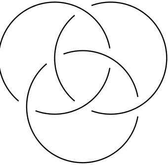
Figure 1.4: Mutant knots. (Images from [64].)

column) and by Schur-Weyl duality correspond to totally symmetric (resp. totally anti-symmetric) representations. Thus, what we call Pn(K;a, q) is the HOMFLY-PT polynomial of K colored by λ=Sn−1.

Even though Pn(K;a, q) provide us with an infinite sequence of two-variable polynomial knot invariants, which can tell apart e.g. the two knots in (1.18), they are still not powerful enough to distinguish simple pairs of knots and links called mutants. The operation of mutation involves drawing a disc on a knot diagram such that two incoming and two outgoing strands pass its boundary, and then rotating the portion of the knot inside the disc by 180 degrees. The Kinoshita-Terasaka and Conway knots shown in Fig. 1.4 are a famous pair of knots that are mutants of one another, but are nonetheless distinct; they can be distinguished by homological knot invariants, but not by any of the polynomial invariants we have discussed so far!

Theorem 1. The colored Jones polynomial, the colored HOMFLY-PT

poly-nomial, and the Alexander polynomial cannot distinguish mutant knots [156], while their respective categorifications can [106,170,207].

1.2 The classical A-polynomial

(33)

defined.

For a knot K, let N(K) _⊂S3 be an open tubular neighborhood of K. Then the knot complement is defined to be

M =ˆ S3_\N(K). (1.23) By construction, M is a 3-manifold with torus boundary, and our goal here is to explain that to every such manifold one can associate a planar algebraic curve

C =_{(x, y)_∈_C2 :A(x, y) = 0_}, (1.24) defined as follows. The classical invariant of M is its fundamental group,

π1(M), which in the case of knot complements is called the knot group. It

contains a lot of useful information about M and can distinguish knots much better than any of the polynomial invariants we saw in §1.1.

Example 3. Consider the trefoil knotK = 31. Its knot group is the simplest

example of a braid group:

π1(M) = ha, b:aba=babi. (1.25)

Although the knot group is a very good invariant, it is not easy to deal with due to its non-abelian nature. To make life easier, while hopefully not giving up too much power, one can imagine considering representations of the knot group rather than the group itself. Thus, one can consider representations of

π1(M) into a simple non-abelian group, such as the group of 2_×2 complex matrices,

ρ:π1(M)→SL(2,C). (1.26)

Associated to this construction is a polynomial invariant A(x, y), whose zero locus (1.24) parameterizes in some sense the “space” of all such representations. Indeed, as we noted earlier, M is a 3-manifold with torus boundary,

∂M =∂N(K)=_e T2. (1.27) Therefore, the fundamental group of ∂M is

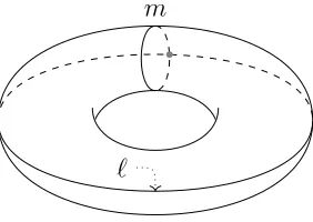
π1(∂M) =π1(T2) =Z×Z. (1.28) The generators ofπ1(∂M) are the two basic cycles, which we will denote bym

(34)

m

`

Figure 1.5: The torusT2 ₌_∂N₍_K_{) for} _K _{= unknot, with cycles} _m _and _`_.

is the cycle that is contractible when considered as a loop in N(K), and `

is the non-contractible cycle that follows the knot in N(K). Of course, any representation π1(M) → SL(2,C) restricts to a representation of π1(T2 = ∂M); this gives a natural map of representations of π1(M) into the space of

representations of π1(∂M).

These cycles are represented in SL(2,_C) by 2 _×2 complex matrices ρ(m) and ρ(`) with determinant 1. Since the fundamental group of the torus is just Z×Z, the matrices ρ(m) and ρ(`) commute, and can therefore be simultane-ously brought to Jordan normal form by some change of basis, i.e., conjugacy by an element of SL(2,_C):

ρ(m) = x ? 0 x−1

!

, ρ(`) = y ? 0 y−1

!

. (1.29)

Therefore, we have a map that assigns two complex numbers to each repre-sentation of the knot group:

Hom(π1(M),SL(2,_C))/conj. _→ _C?_×_C?, ρ _7→ (x, y),

(1.30)

wherexandyare the eigenvalues ofρ(m) andρ(`), respectively. The image of this map is therepresentation variety C _⊂_C?_×

(35)

Example 4. Let K _⊂ S3 _{be the unknot.} _Then _N₍_K_{) and} _M _{are both}

homeomorphic to the solid torus S1_×_D2_{. Notice that} _m _{is contractible as a}

loop in N(K) and ` is not, while the opposite is true in M: ` is contractible and m is not. Since ` is contractible in M, ρ(`) must be the identity, and therefore we havey= 1 for all (x, y)_∈C. There is no restriction on x, so that C( ) = _{(x, y)_∈_C?_×_C? :y= 1_}; (1.31) the A-polynomial of the unknot is therefore

A(x, y) =y₋1. (1.32)

Example 5. LetK _⊂S3 be the trefoil knot 31. Then, as mentioned in (1.25),

the knot group is given by

π1(M) = ha, b:aba=babi, (1.33)

where the meridian and longitude cycles can be identified as follows:

  

m=a,

`=ba2_ba−4_. (1.34)

Let us see what information we can get about the A-polynomial just by con-sidering abelian representations of π1(M), i.e. representations such that ρ(a)

and ρ(b) commute. For such representations, the defining relations reduce to

a2_b ₌ _ab2 _{and therefore imply} _a₌ _b_{. (Here, in a slight abuse of notation, we}

are simply writingato refer toρ(a) and so forth.) Eq. (1.34) then implies that

`= 1 and m=a, so thaty= 1 and xis unrestricted exactly as in Example4. It follows that the A-polynomial contains (y₋1) as a factor.

This example illustrates a more general phenomenon. Whenever M is a knot complement in S3_{, it is true that the abelianization}

π1(M)ab =H1(M)=e Z. (1.35)

Therefore, the A-polynomial always containsy₋1 as a factor,

(36)

In the particular caseK = 31, a similar analysis of non-abelian representations

of (1.25) into SL(2,_C) yields

A(x, y) = (y₋1)(y+x6). (1.37)

To summarize, the algebraic curve C is (the closure of) the image of the rep-resentation variety of M in the representation variety_C?_×

C? of its boundary torus ∂M. This image is always an affine algebraic variety of complex dimen-sion 1, whose defining equation is precisely the A-polynomial [54].

This construction defines the A-polynomial as an invariant associated to any knot. However, extension to links requires extra care, since in that case

∂N(L)₆=_e T2_{. Rather, the boundary of the link complement consists of several}

components, each of which is separately homeomorphic to a torus. There-fore, there will be more than two fundamental cycles to consider, and the analogous construction will generally produce a higher-dimensional character variety rather than a plane algebraic curve. One important consequence of this is that the A-polynomial cannot be computed by any known set of skein relations; as was made clear in Exercise 1, computations with skein relations require one to consider general links rather than just knots.

To conclude this brief introduction to the A-polynomial, we will list without proof several of its interesting properties:

• For any hyperbolic knot K,

AK(x, y)6=y−1. (1.38) That is, the A-polynomial carries nontrivial information about non-abelian representations of the knot group.

• Whenever K is a knot in a homology sphere, AK(x, y) contains only even powers of the variablex. Since in these lectures we shall only consider examples of this kind, we simplify expressions a bit by replacingx2 _with_x_{. For instance,}

in these conventions theA-polynomial (1.37) of the trefoil knot looks like

A(x, y) = (y₋1)(y+x3). (1.39)

• The A-polynomial is reciprocal: that is,

(37)

where the equivalence is up to multiplication by powers of x and y. Such multiplications are irrelevant, because they don’t change the zero locus of the

A-polynomial in _C?_×

C?. This property can be also expressed by saying that the curve C lies in (_C? _×

C?)/Z2, where Z2 acts by (x, y) 7→ (x−1, y−1) and

can be interpreted as the Weyl group of SL(2,_C).

• A(x, y) is invariant under orientation reversal of the knot, but not under re-versal of orientation in the ambient space. Therefore, it can distinguish mirror knots (knots related by the parity operation), such as the left- and right-handed versions of the trefoil. To be precise, if K0 is the mirror of K, then

AK(x, y) = 0 ⇐⇒ AK0(x−1, y) = 0. (1.41)

• After multiplication by a constant, the A-polynomial can always be taken to have integer coefficients. It is then natural to ask: are these integers counting something, and if so, what? The integrality of the coefficients of A(x, y) is a first hint of the deep connections with number theory. For instance, the following two properties, based on the Newton polygon of A(x, y), illustrate this connection further.

• The A-polynomial is tempered: that is, the faces of the Newton polygon of

A(x, y) define cyclotomic polynomials in one variable. Examine, for example, the A-polynomial of the figure-8 knot:

A(x, y) = (y₋1) y2₋(x−2 ₋x−1₋2₋x+x2)y+y2. (1.42)

• Furthermore, the slopes of the sides of the Newton polygon of A(x, y) are boundary slopes of incompressible surfaces† in M.

While all of the above properties are interesting, and deserve to be explored much more fully, our next goal is to review the connection to physics [107], which explains known facts about the A-polynomial and leads to many new ones:

†_{A proper embedding of a connected orientable surface}_F

→M is called incompressible if the induced map π1(F) →π1(M) is injective. Its boundary slope is defined as follows.

An incompressible surface (F, ∂F) gives rise to a collection of parallel simple closed loops in ∂M. Choose one such loop and write its homology class as`p_mq_{. Then, the boundary}

(38)

• The A-polynomial curve (1.24), though constructed as an algebraic curve, is most properly viewed as an object of symplectic geometry: specifically, a holomorphic Lagrangian submanifold.

• Its quantization with the symplectic form

ω = dy

y ∧ dx

x (1.43)

leads to interesting wavefunctions.

• The curve C has all the necessary attributes to be an analogue of the Seiberg-Witten curve for knots and 3-manifolds [67, 89].

As an appetizer and a simple example of what the physical interpretation of the A-polynomial has to offer, here we describe a curious property of the A -polynomial curve (1.24) that follows from this physical interpretation. For any closed cycle in the algebraic curve C, the integral of the Liouville one-form (see (1.49) below) associated to the symplectic form (1.43) should be quantized [107]. Schematically,‡ _I

Γ

logydx x ∈2π

2

·Q. (1.44)

This condition has an elegant interpretation in terms of algebraicK-theory and the Bloch group of ¯_Q. Moreover, it was conjectured in [114] that every curve of the form (1.24) — not necessarily describing the moduli of flat connections — is quantizable if and only if _{x, y_{} ∈} K2(C(C)) is a torsion class. This

generalization will be useful to us later, when we consider a refinement of the A-polynomial that has to do with categorification and homological knot invariants.

To see how stringent the condition (1.44) is, let us compare, for instance, the

A-polynomial of the figure-eight knot (1.42):

A(x, y) = 1₋(x−4₋x−2₋2₋x2+x4)y+y2 (1.45) ‡_{To be more precise, all periods of the “real” and “imaginary” part of the Liouville} one-formθmust obey

I

Γ

log|x|d(argy)−log|y|d(argx) = 0,

1 4π2

I

Γ

(39)

and a similar polynomial

B(x, y) = 1₋(x−6₋x−2₋2₋x2 +x6)y+y2. (1.46) (Here the irreducible factor (y₋1), corresponding to abelian representations, has been suppressed in both cases.) The second polynomial has all of the re-quired symmetries of theA-polynomial, and is obtained from theA-polynomial of the figure-eight knot by a hardly noticeable modification. But B(x, y) can-not occur as theA-polynomial of any knot since it violates the condition (1.44).

1.3 Quantization

Our next goal is to explain, following [107], how the physical interpretation of the A-polynomial in Chern-Simons theory can be used to provide a bridge between quantum group invariants of knots andalgebraic curves that we dis-cussed in§§1.1 and 1.2, respectively. In particular, we shall see how quantiza-tion of Chern-Simons theory naturally leads to a quantizationof the classical curve (1.24),

A(x, y) Aˆ(ˆx,yˆ;q), (1.47) i.e. a q-difference operator ˆA(ˆx,yˆ;q) with many interesting properties. While this will require a crash course on basic tools of Quantum Mechanics, the pay-off will be enormous and will lead to many generalizations and ramifications of the intriguing relations between quantum group invariants of knots, on the one hand, and algebraic curves, on the other. Thus, one such generalization will be the subject of §1.4, where we will discuss categorification and formulate a similar bridge between algebraic curves and knot homologies, finally explain-ing the title of these lecture notes.

We begin our discussion of the quantization problem with a lightning review of some mathematical aspects of classical mechanics. Part of our exposition here follows the earlier lecture notes [66] that we recommend as a complementary introduction to the subject. When it comes to Chern-Simons theory, besides the seminal paper [212], mathematically oriented readers may also want to consult the excellent books [9, 135].

(40)

in time is completely specified by giving 2N pieces of data: the values of the coordinates xi and their conjugate momenta pi, where 1 ≤ i ≤ N. The 2N -dimensional space parameterized by the xi and pi is the phase space M of the system. (For many typical systems, the space of possible configurations of the system is some manifold X, on which the xi are coordinates, and the phase space is the cotangent bundleM =T∗X.) Notice that, independent of the number N of generalized coordinates needed to specify the configuration of a system, the associated phase space is always of even dimension. In fact, phase space is always naturally equipped with the structure of a symplectic manifold, with a canonical symplectic form given by

ω =dp_∧dx. (1.48)

(When the phase space is a cotangent bundle, (1.48) is just the canonical sym-plectic structure on any cotangent bundle, expressed in coordinates.) Recall that a symplectic form on a manifold is a closed, nondegenerate two-form, and that nondegeneracy immediately implies that any symplectic manifold must be of even dimension.

Since ω is closed, it locally admits a primitive form, the so-called Liouville one-form

θ =p dx. (1.49)

It should be apparent that ω =dθ, so that θ is indeed a primitive.

Let us now explore these ideas more concretely in the context of a simple example. As a model system, consider the one-dimensional simple harmonic oscillator. The configuration space of this system is just_R(with coordinatex), and the Hamiltonian is given by

H = 1 2p

2₊1

2x

2_. _(1.50)

Since dH/dt = 0, the energy is a conserved quantity, and since N = 1, this one conserved quantity serves to completely specify the classical trajectories of the system. They are curves in phase space of the form

C : 1 2(x

2 ₊_p2₎

−E = 0, (1.51)

for E _∈ _R+; these are concentric circles about the origin, with radius

(41)

2 1 1 2 x 1

2 3 4

1.0 0.5 0.5 1.0 x

1.0 0.5 0.5 1.0

p

Figure 1.6: On the left, the potential and lowest-energy wavefunction for the simple harmonic oscillator. On the right, the phase space of this system, with a typical classical trajectory.

with a typical trajectory in the phase space. The dashed line represents the lowest-energy wavefunction of the system, to which we will come in a moment. Now, recall that a Lagrangian submanifold C _⊂ (M, ω) is a submanifold such that ω_|_C = 0, having the maximal possible dimension, i.e., dimC =

1

2dimM. (If C has dimension larger than half the dimension of M, the

symplectic form cannot be identically zero when restricted to C, since it is nondegenerate on M.) It should be clear that, in the above example, the classical trajectories (1.51) are Lagrangian submanifolds of the phase space. Moreover, since in this example the degree of the symplectic form ω is equal to the dimension of the phase space,ω is a volume form—in fact, the standard volume form on _R2. We can therefore compute the area encompassed by a trajectory of energyE by integratingωover the regionx2+p2 <2E, obtaining

2πE =

Z

D

dp_∧dx, (1.52)

where D is the disc enclosed by the trajectory C. Therefore, classically, the energy of a trajectory is proportional to the area in phase space it encompasses. How do these considerations relate to quantization of the system? It is well known that the energy levels of the simple harmonic oscillator are given by

E = 1 2π

Z

D

dp_∧dx=_~

n+1 2

(1.53)

(42)

quantum state. Schematically,

# states_∼area/_~. (1.54) This relation has a long history in quantum physics; it is none other than the Bohr-Sommerfeld quantization condition.

Moreover, since ω admits a primitive, we can use the Stokes theorem to write E = 1

2π

Z

D

ω= 1 2π

I

C

θ, (1.55)

since C =∂D and dθ =ω.

We have discussed counting quantum states; what about actually constructing them? In quantum mechanics, we expect the state to be a vector in a Hilbert space, which can be represented as a square-integrable wavefunction Z(x). It turns out that, in the limit where _~ is small, the wavefunction can be constructed to lowest order in a manner that bears a striking resemblance to (1.55):

Z(x)_−−→

~→0

exp i ~ Z x 0 θ+_{· · ·} = exp i ~ Z x 0 √

2E ₋x2_dx₊_{· · ·}

(1.56)

Evaluating the wavefunction in this manner for the lowest-energy state of our system (E =_~/2) yields

Z(x)_≈exp

−₂1 ~

x2+_{· · ·}

. (1.57)

Indeed, exp(₋x2/2_~) is the exact expression for then = 0 wavefunction. We are slowly making progress towards understanding the quantization of our model system. The next step is to understand the transition between the classical and quantum notions of an observable. In the classical world, the observablesxand pare coordinates in phase space—in other words, functions onthe phase space:

x:M _→_R, (x, p)_7→x, (1.58) and so forth. General observables are functions of x and p, i.e., general ele-ments of C∞(M,_R).

In the quantum world, as is well known, x and p should be replaced by oper-ators ˆx and ˆp, obeying the canonical commutation relation

(43)

These operators now live in some noncommutative algebra, which is equipped with an action on the Hilbert space of states. In the position representation, for instance,

ˆ

xf(x) =xf(x), pfˆ (x) =₋i_~ d

dxf(x), (1.60)

where f _∈ L2₍

R). The constraint equation (1.51) that defines a classical trajectory is then replaced by the operator equation

1 2(ˆx

2_{+ ˆ}_p2₎

−E

Z(x) = 0, (1.61)

which is just the familiar Schr¨odinger eigenvalue equation ˆHZ = EZ. Now, unlike in the classical case, the solutions of (1.61) in the position representation will only be square-integrable (and therefore physically acceptable) for certain values of E. These are precisely the familiar eigenvalues or allowed energy levels

E =_~

n+ 1 2

, (1.62)

where n = 0,1,2, . . . . Taking the lowest energy level (n = 0) as an example, the exact solution is Z(x) = exp(₋x2/2_~), just as we claimed above. The reader can easily verify this directly.

All of this discussion should be taken as illustrating our above claim that quantum mechanics should properly be understood as a “modern symplectic geometry,” in which classical constraints are promoted to operator relations. We have constructed the following correspondence or dictionary between the elements of the classical and quantum descriptions of a system:

Classical Quantum

state space symplectic manifold (M, ω) Hilbert spaceH states Lagrangian submanifolds vectors (wave functions)

C ⊂M Z _∈H

observables algebra of functions algebra of operators

f ∈C∞(M) fˆ, acting on H

constraints fi = 0 fˆiZ = 0

(44)

we would also like the correspondence principle to hold: that is, the quantum description should dovetail nicely with the classical one in some way when we take _~_→0.

The correspondence between the classical and quantum descriptions is not quite as cut-and-dried as we have made it appear, and there are a few points that deserve further mention. Firstly, it should be apparent from our discussion of the harmonic oscillator that not every Lagrangian submanifold will have a quantum state associated to it; in particular, only a particular subset of these (obeying the Bohr-Sommerfeld quantization condition, or equivalently, corresponding to eigenvalues of the operator ˆH) will allow us to construct a square-integrable wavefunction Z(x). There can be further constraints on quantizable Lagrangian submanifolds [116].

Secondly, let us briefly clarify why quantum state vectors correspond to La-grangian submanifolds of the classical phase space and not to classical 1-dimensional trajectories, as one might naively think. (In our example of the harmonic oscillator we haveN = 1 and, as a result, both Lagrangian subman-ifolds and classical trajectories are one-dimensional.) The basic reason why Lagrangian submanifolds, rather than dimension-1 trajectories, are the correct objects to consider in attempting a quantization is the following. In quantum mechanics, we specify a state by giving the results of measurements of observ-ables performed on that state. For this kind of information to be meaningful, the state must be a simultaneous eigenstate of all observables whose values we specify, which is only possible if all such observables mutually commute. As such, to describe the state space in quantum mechanics, we choose a “com-plete set of commuting observables” that gives a decomposition of H into one-dimensional eigenspaces of these operators. For time-independent Hamil-tonians, one of these operators will always be ˆH.

However, at leading order in _~, the commutator of two quantum observables must be proportional to the Poisson bracket of the corresponding classical observables. Therefore, if ˆH,fˆi form a complete set of commuting quantum-mechanical observables, we must have

{H, fi}P.B. = 0, (1.63)

(45)

time-evolution of the quantity fi is determined by the equation

dfi

dt +{H, fi}P.B.= 0. (1.64)

As such, the quantum-mechanical observables used in specifying the state must correspond to classically conserved quantities: constants of the motion. And it is well-known that the maximal possible number of classically conserved quantities is N = 1

2dimM, corresponding to a completely integrable system;

this follows from the nondegeneracy of the symplectic form on the classical phase space. ForN >1, then, specifying all of the constants of the motion does not completely pin down the classical trajectory; it specifies anN-dimensional submanifold C _⊂ M. However, it does give all the information it is possible for one to have about the quantum state. This is why Lagrangian submanifolds are the classical objects to which one attempts to associate quantum states. We should also remark that it is still generically true that wavefunctions will be given to lowest order by

Z(x) = exp

i

~

Z x

x0

θ+_{· · ·}

. (1.65)

This form fits all of the local requirements for Z(x), although it may or may not produce a globally square-integrable wavefunction.

Finally, the quantum-mechanical algebra of operators is a non-commutative d