Comparison of Learning Methods in the
Learning Feed-forward Control Setting
Zulkifli Hidayat
M.Sc. Thesis
Supervisors: prof. dr. ir. J. van Amerongen
dr. ir. T.J.A. de Vries
ir. B.J. de Kruif
ir. R. Radzim
January 2004 Report Number 003CE2004
Control Engineering Department of Electrical Engineering
University of Twente P.O. Box 217
Summary
This thesis details the comparison between several learning methods that are to be used in the Learning Feed-forward Control (LFFC) setting. These learning methods consist of the Multilayer Perceptron (MLP), the Radial-Basis Function Network (RBFN), the Support Vector Machine (SVM), the Least Square Support Vector Machine (LSSVM), and the Key Sample Machine (KSM).
The comparison is performed by simulations with respect to reproducibility - the ability to train various training sets from the same function, high dimensional inputs - the ability to train samples from a high dimensional function, and real-world data of a linear motor - the ability to train samples from the motion of a linear motor.
Acknoledgement
Alhamdulillaahi rabbil ´alaamiin, this thesis is finally finished. I would like to thank to people who have
helped me directly or indirectly to finish this thesis. They are:
• prof. Amerongen, who supervised me and provided facilities to work in the Control Engineering
Group and also some useful advices.
• Theo, for supervision and critical comments.
• Bas, from whom the idea of the this thesis came, for his supervision and comments to my results
during my working for the thesis.
• Richie, who made this report much more readable linguistically and also gave a lot of suggestions during writing this report.
• The last but not the least, my parents, who always give support and courage during my life in this world. For them I dedicated this thesis.
I also want to thank to all my friends here, in PPI and especially in IMEA, with whom I share my life, my happiness and sadness. Those make life much better in Enschede. Thanks for all of you.
Contents
Summary i
Acknoledgement iii
1 Introduction 1
1.1 Motivation . . . 2
1.2 Problem Definition . . . 2
1.3 Report Structure . . . 3
2 Learning Methods 5 2.1 Introduction . . . 5
2.2 Artificial Neural Networks . . . 5
2.3 Function Approximation . . . 7
2.4 Multilayer Perceptron . . . 7
2.5 Radial-Basis Function Networks . . . 11
2.6 Support Vector Machine . . . 16
2.7 Least Square Support Vector Machine . . . 19
2.8 Key Sample Machine . . . 20
2.9 Theoretical Comparison of Learning Methods . . . 22
2.10 Summary . . . 24
3 Learning Method Comparison by Simulation 25 3.1 Introduction . . . 25
3.2 Reproducibility Simulation . . . 26
3.3 High Dimensional Inputs Simulation . . . 34
3.4 Off-line Approximation of Linear Motor . . . 40
3.5 Summary . . . 42
4 Conclusions and Recommendations 43 4.1 Conclusions . . . 43
List of Figures
1.1 Block diagram of on-line FEL control . . . 2
2.1 Artificial neural network . . . 6
2.2 Model of a neuron with its inputs . . . 6
2.3 Signal-flow graph highlighting the details of the output neuron . . . 8
2.4 Signal-flow graph highlighting the details of the output neuron connected to the hidden neuronj . . . 10
2.5 Plot of activation functions in the MLP . . . 11
2.6 Plot of RBFs . . . 12
2.7 SVM for Function Approximation . . . 17
2.8 SVM Structure for Function Approximation . . . 17
3.1 Approximated function in reproducibility simulation . . . 26
3.2 Different initial weights reproducibility for the MLP . . . 28
3.3 Reproducibility simulation result of the MLP . . . 29
3.4 Reproducibility simulation result of the RBFN . . . 29
3.5 Reproducibility simulation result of the SVM . . . 31
3.6 Reproducibility simulation result of the LSSVM . . . 31
3.7 Reproducibility simulation result of the KSM . . . 33
3.8 High dimensional inputs simulation results of the MLP and the RBFN . . . 35
3.9 High dimensional inputs simulation results of the SVM, the LSSVM, and the KSM . . . . 36
3.10 Working principle of the linear motor . . . 41
LIST OF TABLES ix
List of Tables
3.1 Number of support vectors of the reproducibility simulation of the SVM . . . 30
3.2 Number of support vectors of the reproducibility simulation of the KSM . . . 32
3.3 Summary of the MSE for the reproducibility simulations . . . 33
3.4 Summary of the number for support vectors of the reproducibility simulations . . . 33
3.5 High dimensional inputs simulation results of the MLP . . . 36
3.6 High dimensional inputs simulation results of the RBFN . . . 37
3.7 High dimensional inputs simulation results of the SVM . . . 37
3.8 High dimensional inputs simulation results of the LSSVM . . . 38
3.9 High dimensional inputs simulation results of the KSM . . . 38
Chapter 1
Introduction
Control problems normally involve designing a controller for a plant based on a model of the plant. This model is in the form of one or more mathematical equations that describe the dynamic behaviour of the plant. A requirement of this model is that it is competent in the problem context. Model competency enables achieving a good working control system according to desired specifications.
A model of a plant can be obtained by the process of system identification. One approach of system identification involves analysing all elements that compose the plant and then deriving a model based on the individual elements. Another approach is assuming the plant as a black-box and then estimating model parameters from input-output data. This approach can be used when there is knowledge of the plant dy-namic structure and external disturbances on the plant are available, but the values of some parameters cannot be determined. When a competent model is difficult to obtain by conventional methods, for exam-ple, the model is so complex that parameters and/or structure cannot be determined, the use of learning control may be considered (Kawato et al., 1987, de Vries et al., 2000).
Learning control is a method of control that applies learning. In systems that implement learning control, there is an element that learns to compensate for system dynamics. Based on how this learning element is used, there exist two types of learning control (Ng, 1997):
• Direct learning control. The learning element is employed to generate the control signal.
• Indirect learning control. The learning element is used to learn the model of the plant. Based on the
resulting model, a controller is designed.
One of the schemes of learning control is Learning Feed-forward Control (LFFC), which is based on Feedback Error Learning (FEL) (de Vries et al., 2000). FEL consists of two parts (Velthuis, 2000):
• Feedback controller. Determines the minimum tracking at the beginning of learning and
compen-sates for random disturbances.
• Feed-forward controller. Maps the reference signal and its derivatives to generate part of the control
signal. When it is equal to the inverse of the plant, the output of the plant will follow the reference.
A block diagram of on-line FEL is shown in Figure 1.1. r is the reference signal,r˙tor(n)are the
reference signal derivatives, C is the controller, andP is the plant. The controllerC can be designed
using methods available in literature. The feed-forward controller in this scheme is designed as a function approximator that tries to imitate the inverse plantP. Signals that are used to train the approximator are
the reference signal and its derivatives (r˙tor(n)) as the inputs, and the output of feedback controllerCas
2 Introduction
C
P
Function approximator
+
+
+
-uc r
¼
r&
) (n
r
Figure 1.1: Block diagram of on-line FEL control
1.1 Motivation
Until recently there have been a number of function approximators developed. Some of them are discussed in this thesis, namely the Multilayer Perceptron (MLP), the Radial-Basis Function Network (RBFN), the Support Vector Machine (SVM), the Least Square Support Vector Machine (LSSVM), and the Key Sample Machine (KSM). Except the KSM, these methods are intended to solve broad spectrum prob-lems (Haykin, 1999, Cristianini and Shawe-Taylor, 2000), for example classification, image processing, and regression/function approximation. Only that the KSM is firstly developed to be used in the learning feed-forward control setting (de Kruif, 2003).
In general, no method is superior for all applications. Each has its advantages and disadvantages when applied to a certain problem. This also applies to learning control. Velthuis (2000) mentions the characteristics of a function approximator that are suitable for use in control. These characteristics are:
• Small memory requirement in implementation
• Fast calculation for input-output adaptation and prediction
• Convergence of the learning mechanism should be fast • The learning mechanism should not suffer from local minima • The input-output relation must be locally adaptable
• Good generalising ability
• The smoothness of the approximation should be controllable
1.2 Problem Definition
Based on the fact that every learning method has advantages and disadvantages for a certain problem, the following question which forms the basis for this thesis arises: What is the performance comparison of learning methods when used as a function approximator in LFFC?
This question can now be divided into a number of questions, being: 1. How does a learning method work as a function approximator?
This question should be answered by studying literature about learning methods. 2. How to compare all learning methods as function approximators?
This question should be answered by finding aspects that can be compared. 3. How good are the performances of the learning methods compared to each other?
1.3 Report Structure 3
1.3 Report Structure
The structure of the report is as follows:
Chapter One details the background, motivation, and problem definition of this thesis.
Chapter Two presents an overview of all learning methods. Each method is presented followed by detail of the functioning of the method.
Chapter Three describes aspects used to show the performance comparison of function approximators, followed by simulation results of comparisons. Discussion of the results is presented.
Chapter 2
Learning Methods
2.1 Introduction
This chapter gives an overview of the learning methods that are compared in this thesis. Those methods are backpropagation used in the Multilayer Perceptron (MLP), the Radial-Basis Function Network (RBFN), the Support Vector Machine (SVM), the Least Square Support Vector Machine (LSSVM), and the Key Sample Machine (KSM).
Firstly an introduction to the Artificial Neural Network (ANN) is given. Then each learning method will be briefly introduced followed by an insight into its working principle. After all methods have been presented, their working principle will be compared and discussed.
2.2 Artificial Neural Networks
The ANN is a method that is inspired by the works of a human brain. It uses weighted connections of processing elements called neurons into which signals are fed and processed to yield outputs. The connector is called a synaptic connector. For specified input signals, outputs of the ANN depend on the weight of the synaptic connectors, the structure of the network, and the function inside the neurons. In this report, the term ’network’ will refer to the ANN as well.
Before going further into detail of the structure and elements of the ANN, the basic working principle will be explained. There are two processes occurring in an ANN: The first is signals from the input layer are transmitted to the output layer. In this process, there is no change in the network and the propagated signal is called function signal. This process is called prediction. The second is learning or training. In this process, the parameters of the network are adapted or trained based on the output and will be different for different types of ANNs. Both process are performed iteratively and ended when one or more stopping criterion are fulfilled.
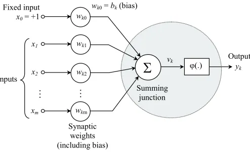
In general, the structure of an ANN can be illustrated as shown as in Figure 2.1. As shown in the figure, the structure consists of an input layer, one or more hidden layers, and an output layer. In the input layer there is no neuron. Therefore signals are propagated directly to the right, to the hidden layer. This hidden layer contains one or more neurons and it is possible to have more than one hidden layer in a network. The last part is the output layer (most right of figure). The number of neurons in the output layer depends on the number of outputs of the network.
Consider a model of a neuron with its inputs as shown in Figure 2.2. The neuron (grey part) receives the weighted signals from the synaptic connectors as its input. These signals are then summed and processed using the so-called activation function. This activation function can be either linear or non-linear. The output is then propagated to the next layer until the output layer. A different activation function used in the neurons can possibly lead to different naming of the ANN.
6 Learning Methods
¼
Input signal (stimulus)
Output signal (response)
Input layer
One or more hidden layer
Output layer
¼
¼
¼
¼
¼ ¼
Neuron unit Synaptic
connector
Figure 2.1: Artificial neural network (Haykin, 1999)
wk0
wk1
wk2
Fixed input x0= +1
x1
x2
wk0=b
Figure 2.2: Model of a neuron with its inputs (Haykin, 1999)
pair of equations as follows
vk= m X
j=1
wkjxj+w0bk (2.1)
and
yk=ϕ(vk) (2.2)
wherex1, x2, . . . , xmare input signals,wk1, wk2, . . . , wkmare the synaptic weights of the neuronk,vkis
the output of the linear combination of input signals,bkis the input bias,ϕ(.)is the activation function, and
yk is the output signal. Input bias is a constant input signal which is set to a value of +1 and its amplitude
to neuron input is determined by the weight of its synaptic weight. Activation functions that can be used inside a neuron are the threshold function, piecewise linear function, and sigmoid function.
There are two classes of networks that can be constructed from these neurons:
1. Feed-forward networks. In this structure, input signals are fed from the input layer and then
for-warded to the output layer.
2. Recurrent networks. Different from previous, in this structure, some of the network outputs are fed
back to the input layer.
2.3 Function Approximation 7
1. Learning with a teacher. The training of the network in this class is performed based on examples.
The error between the network output and the examples are used for training. The objective is to minimize the error. An example of this class is the MLP.
2. Learning without a teacher. There is no example to follow in this method. An example of this class
is the Kohonen self-organising.
In this report all of the networks discussed are in the class offeed-forward networksthatlearn with
teacher.
2.3 Function Approximation
Function approximation involves approximating a relation between the input and output data from a set of training samples or data. Given a set of training samples{xk, dk}k=1,...,N wherexk is the input vector
anddk is the corresponding desired value for samplek, a function approximator will map x → yˆ(x).
This mapping can be evaluated for any value ofxthat is not part of a training set. The performance of a
function approximator is measured from the error between the output of the approximator and the target of the training samples.
A problem that is related with the training data is noise. In most cases, real-world data is not noise-free. This noise may reduce the performance of the approximator. This means if the difference between the approximator outputyˆk anddk, or the square of the training error, is zero, the approximator follows
corrupted data which are not the real function value. This problem is known as overfitting.
Overfitting will cause low generalisation performance (Haykin, 1999). Generalisation is one of the performance measures of a function approximator that is about the ability to predict values from data that are not in the training data. In the case of overfitting, the approximator memorises the learning data and does not learn.
Another related problem is approximating a function with high dimensional inputs. This problem is known as Curse of Dimensionality. The problem is the higher the dimensionality of the approximated function, the more complex the computation needed and therefore more training data is required to keep the level of accuracy (Haykin, 1999).
In practice, training of a function approximator involves two steps (Prechelt, 1994):
1. Training
2. Validation
Each step uses a different data set. This method is called Cross-Validation. Therefore, to use this training method, the training set has to be divided into two subsets. The first subset is used as a training set for the approximator and then generalisation performance is checked using the second subset. Detail of this method and its variations can be found in (Prechelt, 1994, Kohavi, 1995). This cross-validation is applied in this thesis.
The next part of this report will discuss the MLP using back-propagation learning followed by the RBFN, the SVM and the LSSVM, respectively and the KSM.
2.4 Multilayer Perceptron
8 Learning Methods
x0= +1
w0= -b(n)
Output neuron
Figure 2.3: Signal-flow graph highlighting the details of the output neuron (Haykin, 1999)
2.4.1 Back-Propagation Algorithm
The most popular training method for the MLP is Back-Propagation Learning or Backprop for short. In this method there are two steps involved which are performed iteratively, the forward and the backward step. In the forward step or prediction, input signals are propagated through the network layer by layer until a set of output signals are produced while all synaptic weights in the network are kept fixed.
These output signals are then compared to the desired signals. The differences (error signals) are then propagated backward through the network from the output layer to input layer against the direction of synaptic connection. In the backward step or correction, the synaptic weights are adjusted according to the error correction rule to make the actual response of the network closer to the desired response. In this step, the learning process is performed. These two steps are repeated until a stopping criteria is reached.
The correction step begins from calculation of the output error of neurons in the output layer of a network. If we assume that only one neuron exists, the output error at timencan be calculated from
e(n) =d(n)−y(n) (2.3)
The instantaneous value of error energy is defined as
E(n) = 1
2e
2(n) (2.4)
If there areNnumber of training samples available, the average square of the error energy can be calculated as
Eav(n) = 1
N
N X
n=1
E(n) (2.5)
It can be seen that both functions above, (2.4) and (2.5), are functions of free parameters, i.e. synaptic weights and bias levels, and (2.5) represents the cost function as a measure of learning performance for a given training set. The objective of the learning process is to adjust the free parameters to minimizeEav.
Consider Figure 2.3 which highlights the detail of an output neuron. The sum of input signalxi,v(n),
is written as
v(n) =
m X
i=0
wi(n)xi(n) (2.6)
wheremis the total number of inputs (including bias). Output signaly(n)at iterationncan be written as
2.4 Multilayer Perceptron 9
In the Backprop algorithm, the correction factor of the synaptic weightwi(n),∆wi(n), is proportional
to the partial derivative∂E/∂wi. Using the chain rule from Calculus,∂E/∂wican be calculated from
∂E(n)
∂wi(n)
=∂E(n)
∂e(n)
∂e(n)
∂y(n)
∂y(n)
∂v(n)
∂v(n)
∂wi(n)
(2.8)
which results in
∂E(n)
∂wi(n)
=−e(n)ϕ0(v(n))x
i(n) (2.9)
The correction factor∆wi(n)employed towi(n)is defined by the delta rule as follows
∆wi(n) =−η
∂E(n)
∂wi(n)
(2.10)
where η is the learning-rate parameter. The minus sign accounts for gradient descent in weight space.
(2.10) can be rewritten as
∆wi(n) =ηδ(n)xi(n) (2.11)
where the local gradientδ(n), which is points to required changes in synaptic weight, is defined by
δ(n) =e(n)ϕ0(v(n)) (2.12) Calculation of the local gradient in (2.12) applies only if the neuron is in the output layer. For a neuron in the hidden layer, consider Figure 2.4. For neuronjas a hidden node, the local gradient is
δj(n) = −
∂E(n)
∂xj(n)
∂xj(n)
∂vj(n)
= − ∂E(n)
∂xj(n)
ϕ0
j(vj(n)) (2.13)
The first term of (2.13) can be calculated as
∂E(n)
∂xj(n)
=−δ(n)wj(n) (2.14)
Local gradientδj(n)can be written as
δj(n) =ϕ0j(vj(n))δ(n)wj(n) (2.15)
whereδis the local gradient calculated previously in (2.12).
The training time using the method derived above is long. One heuristic way to increase the learning speed is using a momentum term. The delta rule in (2.11) can be generalized by adding a momentum term that is defined as the previous synaptic weight multiplied by a constant, so (2.11) becomes
∆wji(n) =α∆wji(n−1) +η δj(n)yi(n) (2.16)
whereαis the momentum constant which is usually positive.
The MLP has two modes of training, namely:
1. Batch mode. Synaptic weight adaptation is computed after all training samples have been presented to the network. One phase of feeding all training samples is calledepoch.
10 Learning Methods
+1
z0= +1
wj0=bj(n)
Neuronj
Figure 2.4: Signal-flow graph highlighting the details of the output neuron connected to the hidden neuron
j(Haykin, 1999)
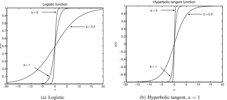
1. Logistic function. This function has the form as follows
ϕj(vj(n)) =
1
1 + exp(−a vj(n))
a >0,−∞< vj<∞ (2.17)
Its derivative with respect tovj(n)is
ϕ0
j(vj(n)) =
a exp(−a vj(n))
[1 + exp(−a vj(n))]2
(2.18)
Usingyj(n) =ϕj(vj(n))
ϕ0
j(vj(n)) =a yj(n)[1−yj(n)]
ϕ0
j(vj(n))is maximum atyj(n) = 0.5and minimum atyj(n) = 0oryj(n) = 1. The amount of
change in synaptic weight of the network is proportional to the derivativeϕ0
j(vj(n))so that a large
change in synaptic weight occurs for neurons into which the input signals are in their mid-range. This contributes to the functions stability as a learning algorithm. A plot of the logistic function is shown in Figure 2.5(a).
2. Hyperbolic Tangent Function. This function is defined by
ϕj(vj(n)) =atanh(b vj(n)) a, b >0 (2.19)
Its derivative with respect tovj(n)is
ϕ0
j(vj(n)) =
b
a[a−yj(n)][a+yj(n)] (2.20)
A plot of the hyperbolic tangent function is shown in Figure 2.5(b).
2.4.2 Discussion
In one view the MLP can be seen as a mapping from input space to output space via one or more feature spaces in hidden layers. The dimension of this mapping in the feature spaces is determined by the number of neurons in each hidden layer and the number of feature spaces depend on the number of hidden layers.
2.5 Radial-Basis Function Networks 11
−200 −15 −10 −5 0 5 10 15 20 0.1 0.2 0.3 0.4 0.5 0.6 0.7 0.8 0.9
1 Logistic function
x
y(x)
a = 3
a = 1
a = 0.2
(a) Logistic
−20 −15 −10 −5 0 5 10 15 20
−1 −0.8 −0.6 −0.4 −0.2 0 0.2 0.4 0.6 0.8 1
Hyperbolic tangent function
x
y(x)
b = 3
b = 1
b = 0.2
(b) Hyperbolic tangent,a= 1
Figure 2.5: Plot of activation functions for different parameters
the contribution of a synaptic weight to the error, the bigger the modification of its value in the adaptation process and vice versa.
The role of learning parameterηis to determine the quantity of the synaptic weight correction and its
value is between 0 and +1. Settingηtoo large can cause instability to the training process, whereas setting ηtoo small will lengthen the training time.
One drawback of the MLP learning is the slow learning time. One heuristic way to increase the learning time is by adding a momentum term, see Page 9. When the sign of a synaptic correction is always the same during the iteration, the momentum has the effect of accelerating the learning, however if the sign of the correction is changed during the iteration, the momentum gives a stabilizing effect (Haykin, 1999).
Another drawback is related with the initial value of the synaptic weights which are set small and randomly. For different initial weights the result of the approximation can be different. This can be seen if an MLP is trained and simulated with the same training data but different initial weights. There will be conditions where the approximation result of a network is worse than others. This problem is known as the local minima problem.
In dealing with curse of dimensionality, no further information can be found except from (Haykin, 1999) which states that the MLP suffers from curse of dimensionality since its complexity increases with an increase in input dimensionality.
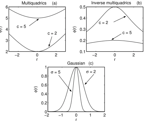
2.5 Radial-Basis Function Networks
The RBFN is a feed-forward neural network that uses a radial-basis function in its processing element (neuron). In its structure it has an input layer, an output layer and one or more hidden layers, but one hidden layer is most common.
Before proceeding into the discussion about the RBFN, it is necessary to know the definition of a radial-basis function (RBF). A RBF is a function whose output is symmetric around an associated center
µ(Ghosh and Nag, 2001). Those that are of particular interest in the RBFN are (Haykin, 1999):
1. Multiquadrics
φ(r) = r2+c212 for some c >0
2. Inverse multiquadrics
φ(r) = 1
(r2+c2)12
12 Learning Methods
−2 0 2
2 3 4 5 6 Multiquadrics r φ (r)
−2 0 2
0.1 0.2 0.3 0.4
0.5 Inverse multiquadrics
r
φ
(r)
−20 −1 0 1 2
0.2 0.4 0.6 0.8 1 Gaussian r φ (r)
c = 5
c = 2
c = 2
c = 5
σ = 2
σ = 5
(a) (b)
(c)
Figure 2.6: Plot of RBFs φ(r) with different parameters: (a)Multiquadrics (b)Inverse multiquadrics (c)Gaussian
3. Gaussian function
φ(r) = exp
− r
2
2σ2
for someσ >0
Among the above functions, the Gaussian is most commonly used. The shape of all functions above is illustrated in Figure 2.6.
The application of the RBFN as a function approximator can be derived from solving the strict inter-polation problem as follows
Definition 1 (Interpolation Problem) (Haykin, 1999) Given a set of N different points{xi ∈Rm0|i=
1,2, . . . , N}and a corresponding set of N real numbers{di ∈R1|i= 1,2, . . . , N}find a function F that satisfies the interpolation condition:
F(xi) =di, i= 1,2, . . . , N (2.21)
A RBF technique to solve this problem is by choosing a functionFthat has the following form:
F(x) =
N X
i=1
wiφ(kx−xik) (2.22)
where{φ(kx−xik)|i= 1,2, . . . M}is a set of RBFs andM =N, namely the number of RBFs is the same as the number of data, and notation in (2.22)k.kis usually Euclidean.
From (2.21) and (2.22), a set of simultaneous linear equations for unknown coefficients is obtained:
φ11 φ12 · · · φ1M
φ21 φ22 · · · φ2M
... ... ... ...
φN1 φN2 · · · φN M
w1 w2 ... wN = d1 d2 ... dN (2.23) where
2.5 Radial-Basis Function Networks 13
In matrix form, (2.23) can be written as
Φw=x (2.25)
whereN−by−1vectorsdandware the desired response vector and linear weight vector respectively,N
is the size of the training sample,M is the number of RBFs, andΦis anN−by−M matrix with element
φjiwritten as
Φ={φji|i= 1,2, . . . , N, j= 1,2, . . . , M}
IfΦis nonsingular, vectorwcan be calculated as
w=Φ−1x (2.26)
Singularity ofΦcan be avoided by a set of training data whose elements/points are different, so that
all rows and columns are linearly independent.
Once the weights have been determined, they can be used for approximation by feeding the validation data set. If the training data follow an unknown functionyand its estimate is denoted byyˆ, the
approxi-mation of new dataxk, k= 1, . . . , Pcan be written as
φ11 φ12 · · · φ1M
φ21 φ22 · · · φ2M
... ... ... ...
φP1 φP2 · · · φP M
w1 w2 ... wM = ˆ y1 ˆ y2 ... ˆ yP (2.27) where
φki=φ(kxk−xik), i= 1,2, . . . , M k= 1,2, . . . , P
In the strict interpolation above the number of RBFs are as many as the data points, which may end up with overfitting. To avoid such a problem, the number of RBFs used is less than the number of data, i.e.
M < N. This scheme is known as the Generalised RBFN (Haykin, 1999).
2.5.1 Training Radial-Basis Function Networks
After defining the network, as it is in other ANNs, the RBFN needs training. The parameters that can be trained in this network are RBFs’ parameters (centres and widths), and the synaptic weights. Different from the MLP, training of this network can be performed in three different ways:
1. Training with fixed randomly selected centres and fixed equal width. This way the training is only searching for the synaptic weights.
2. Self-organised selection of centres. The centres and width of the RBF are sought first and once they are determined the synaptic weight is calculated.
3. Supervised selection of centres. All of the parameters are trained simultaneously using gradient descent optimisation.
All these training methods are explained in detail in the subsequent sub-sections.
Fixed centres selected at random
In this training method, firstly, the centers of a RBF network are located randomly and are then kept fixed during training. Assume that Gaussian RBFs whose standard deviation is fixed according to the spread of the centers are used, namely
G kx−µik2= exp
− m1
dmax
kx−µik2
, i= 1,2, . . . , m1
14 Learning Methods
The parameters that need to be trained in this way are the weights in the output layer. This can be solved by using the pseudoinverse method
w=G+d (2.28)
wheredis the desired response vector in the training set,G+is the pseudoinverse ofG. The pseudoinverse
for a nonsquare matrix is functionally equal with the inverse of a square matrix.
Calculation of the pseudoinverse of any matrixAdepends on three conditions as follows (Golub and
Loan, 1996):
• Columns inAare linear independent, pseudo inverse ofAis defined as
A+= ATA−1AT (2.29)
• Rows inAare linear independent, pseudoinverse ofAis defined as
A+=AT ATA−1 (2.30)
• Neither rows nor columns inAare linear independent, pseudoinverse ofAis calculated using
Sin-gular Value Decomposition (SVD).
Self-organised selection of centers
This method consists of two steps:
1. Estimating the appropriate locations for the centers of RBFs in the hidden layer. 2. Estimating the linear weight of the output layer.
The center locations of the RBFs and their common widths are computed using a clustering algorithm, for example, thek-means clustering algorithm or self-organising feature map from Kohonen. Once the
cen-ters are identified the computation of the weights of the output layer can be performed using pseudoinverse as it is done in the previous subsection.
Supervised selection of centers
In this approach, the training of the RBFN takes the most general form, i.e. all of the free parameters of the network undergo a supervised learning process. This process is a kind of error learning that is implemented using the gradient descent procedure. The first step in the development of the learning procedure is to define the instantaneous value of the cost function
E(n) = 1
2
N X
j=1 e2
j (2.31)
whereN is the size of the training sample used to do the training andejis the error signal defined by
ej = dj−F∗(xj)
= dj− M X
i=1
wiG(kxj−µikCi) (2.32)
A Gaussian RBFG(kxj−µikCi)centered atµiand with norm weighting matrixCmay be expressed
as
G(kxj−µikCi) = exp−(x−µi)TCTC(x−µi)
= exp
−1
2(x−µi)
TΣ−1(x−
µi)
2.5 Radial-Basis Function Networks 15
where
1 2Σ
−1=CTC
is the spread of the RBF.
The requirement is to find the three parameterswi,µi, and,Σ−1 to minimiseE. The result is
sum-marised as follows:
1. Linear weights (output layer)
∂E(n)
∂wi(n)
= − N X
j=1
ej(n)G(kxj−µµµikCi)
wi(n+ 1) = wi(n)−η1 ∂E(n)
∂wi(n)
i= 1,2, . . . , m1
2. Position of centers (hidden layer)
∂E(n)
∂µµµi(n)
= −2wi(n) N X
j=1
ej(n)G0(kxj−µµµikCi)Σ
−1
i [xxxj−µi]
µµµi(n+ 1) = µµµi(n)−η2 ∂E(n)
∂µµµi(n)
i= 1,2, . . . , m1
3. Spreads of centers (hidden layer)
∂E(n)
∂Σ−1
i (n)
= wi(n) N X
j=1
ej(n)G0(kxj−µµµikCi)Oji(n)
Oji(n) = [xj−µµµi][xj−µµµi]T
Σ−1
i (n+ 1) = Σ−
1
i (n)−η3
∂E(n)
∂Σ−1
i (n)
2.5.2 Discussion
The RBFN, from its name, uses RBFs to construct the input-output nonlinear mapping, instead of using a sigmoidal nonlinear function as in the MLP. The RBF is called a kernel function which maps the input into the feature space. It can be seen that the input space should be covered by the RBFs that are distributed inside it.
The RBFN works by calculating the distance between the input data and the center of the RBF. The nearer the input with the center, the closer the output of the RBF to +1. When one input is very close to one of the neuron centres, its output dominates the output of the network while the output of other neurons is much smaller. This shows that the RBF constructs a local approximation for each neuron. Furthermore, a neuron directly corresponds to the mapping of an interval input-output. Thus, it is enough to use only one hidden layer in a RBFN.
Input space coverage is determined by the width and the number of RBFs. If the RBFs’ widths are large and they almost overlap each other, there are inputs that activate more than one RBF so that the columns represented by those RBFs are closer to being linear dependent. On the other hand if the distance is too far, there will be data that do not activate any RBF so that the network is not trained at that region. However, using more RBFs of small width will make the network behaviour closer to strict interpolation which means overfitting can occur.
16 Learning Methods
Training with random centre positions does not give optimal results since the results will be different for each run. Alternatively, visual design can be considered if the input dimension is less than three. The RBFs’ positions can be arranged in such a way that they are located on positions that give less error. Nevertheless it is hard to apply such a design method since, in general, real-world data has a large dimension.
Self-organised selection of centres puts the centres of a certain width on the centres of a group of data. It is expected that the error contributions from data in those groups are small, since they are close to the RBFs centres. In this training method, blank spots that are not covered by the RBFs possibly occur.
In the case of supervised selection of centres and width, since this method uses gradient descent opti-misation, it could probably be that the error minimisation with respect to both parameters is trapped into local minima. The other disadvantage is that the training time is long. But the result of this training, if the training is not trapped into local minima, is optimal in the sense that the RBF parameters and the synaptic weights are set to give minimal error.
In the case of high dimensional function approximation, as it is in the MLP, this method also suffers from curse of dimensionality (Haykin, 1999).
2.6 Support Vector Machine
The Support Vector Machine (SVM) is a relatively new method developed based on statistical learning theory proposed by Vapnik (Smola and Sch¨olkopf, 1998).
In this section, the function to be approximated is written as
f(x) =wTϕ(x) +b (2.34)
In the SVM, the goal of the approximation is to find a functionf(x)that has at mostε deviation from
the actual output of the approximator for all training data and, at the same time, be as flat as possible. Flat means thatwshould be small and one way to ensure flatness is by minimising||w||2. The deviation has a
relation with theε-insensitive loss function which is defined as (Haykin, 1999)
Lε =
|d−yˆ| −ε for|d−yˆ| ≥ε
0 otherwise (2.35)
wheredis the target,yˆis the approximated value. (2.35) says that if the difference between the target and the approximated value is less thanε, it is ignored.
The approximation problem can be formulated as a convex minimisation problem as follows (Smola and Sch¨olkopf, 1998):
Φ(w) =1 2w
Tw
subject to
di−wTϕ(xi)−b ≤ ε i= 1,2, . . . , N
wTϕ(xi) +b−di ≤ ε i= 1,2, . . . , N
To allow some errors, slack variablesξandξ∗are introduced. The minimisation problem then becomes
Φ(w, ξ, ξ0) = 1
2w
Tw+C
N X
i=1
(ξi+ξ0i) !
(2.36)
subject to
di−wTϕ(xi)−b ≤ ε+ξi i= 1, . . . , N (2.37)
wTϕ(xi) +b−di ≤ ε+ξi0 i= 1, . . . , N (2.38)
2.6 Support Vector Machine 17
x y
e x
Figure 2.7: SVM for 1D Function Approximation
(.)
j(.)
S
¼ ¼
x1 x2 x3 xM
x a1
a2 a3 aM
b
Input vector Support vector Mapped vector Dot product
j(.) j(.) j(.) j(.)
(.) (.) (.)
yˆ
Figure 2.8: SVM Structure for Function Approximation
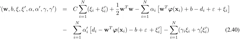
An illustration of the SVM for 1D function approximation can be seen in Figure 2.7. The Lagrangian function can then be defined as (Haykin, 1999)
J(w, b, ξ, ξ0, α, α0, γ, γ0) = C
N X
i=1
(ξi+ξi0) +
1 2w
Tw
− N X
i=1 αi
wTϕ(xi) +b−di+ε+ξi
− N X
i=1 α0
i
di−wTϕ(xi)−b+ε+ξi0
− N X
i=1
(γiξi+γi0ξi0) (2.40)
whereαiandα0iare the Lagrange multipliers. The requirement is to minimiseJ(w, ξ, ξ0,
18 Learning Methods
The corresponding dual problem can be written as (Haykin, 1999)
Q(αi, αi0) = N X
i=1
di(αi−α0i)−ε N X
i=1
(αi−α0i)
− 1
2
N X
i=1
N X
j=1
(αi−α0i)(αj−α0j)K(xi−xj) (2.41)
subject to
N X
i=1
(αi−α0i) = 0 (2.42)
0≤αi≤C, i= 1,2, . . . , N (2.43)
0≤α0
i≤C, i= 1,2, . . . , N (2.44)
whereK(xi,xj)is the inner-product kernel defined to fulfill Mercer’s theorem:
K(xi,xj) =ϕ(xi)Tϕ(xj)
The approximation for the new value dataxnis written as follows (Haykin, 1999)
F(xn,w) = wTxn+b
=
N X
i=1
(αi−α0i)K(xn,xi) +b (2.45)
The SVM structure for function approximation is shown in Figure 2.8. The constantbcan be calculated
from (Smola and Sch¨olkopf, 1998)
b=yi−wTϕ(xi)−ε forαi∈(0, C)
b=yi−wTϕ(xi) +ε forα0i∈(0, C)
(2.46)
2.6.1 Discussion
As it is illustrated in Figure 2.7, due to the ε-insensitive loss function, the SVM works by making a band/tube with diameter2ε around the approximated function. The tube is shaped in the training error optimisation process and in this process, error from samples inside the tube are ignored. The error is optimised indirectly in the feature space using the kernel function in the input space, i.e. by minimising the innerproduct of the kernel’s output. It is expected that the nonlinear function to approximate, can be mapped linearly in the feature space. At the end of training there are some samples outside the tube, known
asSupport Vectorsand they are used for prediction.
It can be said that the number of support vectors depends on the tube’s width which is determined byε while the parameterC controls the trade-off between the training error and the magnitude of the weights. This parameterC determines the weight of error minimisation such that a largerC will force the optimisation process to minimise the slack variables. Therefore it can be seen that both parameters control the result of the approximation and also the number of support vectors. The difficulty in this method emerges as to how to determine both parameters since they are independent and should be tuned simultaneously.
With respect to computation, it is desired to have a small number of support vectors in the model such that the prediction can be performed with less calculation while keeping training error small, and good generalisation. A small number of support vectors is also desired to avoid overfitting.
2.7 Least Square Support Vector Machine 19
2.7 Least Square Support Vector Machine
The Least Square Support Vector Machine (LSSVM) is a variant of the SVM explained previously. This method is developed by Suykens et. al. (Suykens, 2000).
The difference of the LSSVM is in its cost function. It has a quadratic cost functionJwhich is defined
as
J(w, e) = 1 2w
Tw+γ1
2 N X i=1 e2 i (2.47) subject to
di=wTϕϕϕ(xi) +b+ei, i= 1,2, . . . , N (2.48)
whereγis a constant andeiis the error between the estimated valueyˆiand the the desired valuedi.
The Lagrangian of the optimisation problem can be expressed as
J(w, e, b, α) =1 2w
Tw+γ1
2
N X
i=1 e2k−
N X
i=1
αiwTϕϕϕ(xi) +b+ei−di (2.49)
whereαis the Lagrange multiplier.
As in the SVM, the error has to be optimised for which the condition for optimality is fulfilled, by setting the derivatives ofJ(w, e, b, α)with respect tow, b, ei, andαiequal to zero.
The optimisation result can be written in matrix form as follows (Suykens, 2000)
0 1
1 ϕϕϕ(xi)Tϕϕϕ(xj) +γ−1
b αi = 0 di
i, j= 1,2, . . . , N
and in more compact form as in (Suykens, 2000)
0 ¯1T
¯
1 ΩΩΩ +γ−1I αααb = 0 d (2.50)
whered,¯1, andαare anN×1array, namely
d = [d1 d2 · · · dN]T
¯
1 = [1 · · · 1]T
ααα = [α1 α2 · · · αN]T
and
Ω = ϕϕϕ(xi)Tϕϕϕ(xj), i, j= 1,2, . . . , N
= K(xixj)
The values ofαandbcan be calculated by solving (2.50). The approximation equation for the new
value dataxnis written as
F(xn) = N X
i=1
αiK(xn,xi) +b (2.51)
In (2.51), the new value data is calculated without using weight vectorwsince it vanished when the
cost functionJ in (2.49) was differentiated with respect tow.
2.7.1 Discussion
20 Learning Methods
γ, that determines how low the error is minimised which then consequently determines the roughness of the estimation. The larger the value ofγthe smaller the cost function but the coarser estimation is obtained. Coarse estimation means the model resulting from training includes a lot of samples or support vectors.
After fulfilling the condition for optimality, the optimisation problem is represented by a set of simulta-neous linear equations. By solving these equations, the LSSVM looses sparseness in the solution. To force a sparse solution, the process of pruning is performed after training. This process removes some support vectors while the training performance is measured to track its decrease. Pruning is continued as long as the new performance is not less than specified.
2.8 Key Sample Machine
The Key Sample Machine (KSM) is developed by Kruif (de Kruif and de Vries, 2002) from Least Squares (LS) regression. The overview of this method begins with an explanation of LS, primal and dual LS and follows with how the KSM differs from LS regression.
Given a set of input-output data pairs as the samples and a set of indicator functions fk(x), k =
1, . . . , P, the LS method searches for parameters wk, k = 1, . . . , P to fulfill the linear relation in the
equation
ˆ
y(x) =w1f1(x) +w2f2(x) +· · ·+wPfP(x) (2.52)
whereyˆis the approximation ofy, by minimising the sum-of-square approximation error(y−yˆ)over all
samples. The form of the indicatorfk(x), k= 1, . . . , Pcan be constant, linear, or nonlinear, that maps the
input space to a feature space. In matrix form, (2.52) can be formulated as follows
ˆ
y=Xw (2.53)
Matrix X is defined as the indicator for all N samples and target values respectively, and can be
formulated as X=
f1(x1) f2(x1) · · · fP(x1)
f1(x2) f2(x2) · · · fP(x2)
... ... ...
f1(xN) f2(xN) · · · fP(xN)
, w=
w1 w2 ... wP
where the subscript ofxdenotes the sample number. The LS problem can be solved by primal and dual
optimisation approaches.
2.8.1 Primal form
In the primal form, the minimisation problem is expressed as
min
w
1 2λkwk
2 2+
1
2kXw−dk
2
2 (2.54)
wheredis the target vector corresponding to the samples.
The term 1
2kwk22is included to decrease the variance of thew’s at the cost of a small bias andλis the
regularisation parameter. The solution of the above minimisation can be found by setting the derivative of (2.54) equal to zero, resulting in
λI+XTXw=XTd (2.55)
In this form, (2.55) requires that the number of training data is equal to or more than the number of indicators. If this requirement is not fulfilled, the matrixXTXwill be singular.
The estimationF(x)for a new inputxn, denoted byyˆis
ˆ
y=
N X
i=1
2.8 Key Sample Machine 21
2.8.2 Dual form
Another way to solve the minimisation problem in the primal form is by using its dual form. This is done by the minimisation
min
w
1 2λw
Tw+1
2e
Te (2.57)
with equality constraint
d=Xw+e
whereeis a column-vector containing the approximation error for all samples.
The Lagrangian of the problem is
J(w,e,α) =1
2λw
Tw+1
2e
Te−
αT(Xw+e−d)
The vectorαcontains the Lagrangian multiplier with the dimensionN, the number of data samples. The problem can be solved by setting the derivatives of the Lagrangian with respect tow,e, andαequal
to zero.
The solution can be formulated in the primal variablew or in the dual variableααα. The solution in primal form, which is the same as in the previous section, can be seen in (2.56).
In dual form, the solution is given by
λI+XXTα = d (2.58)
w = XTα (2.59)
The estimate of a new inputxncan be calculated as
ˆ
y = f(xn)XT
λI+XXT− 1 d (2.60) = N X i=1
hf(xn), f(xi)iαi (2.61)
This form requires that all of the rows of matrixXare linearly independent, which means data with the
same value is not allowed (leads to singularity ofXXT). Different to the primal form, dual form does not
have problems with smaller training data compared to indicator functions.
2.8.3 Primal and Dual Combination
From (2.56) it can be seen that the calculation of new data input in primal form uses thef(x)explicitly. On the other hand, in dual form, the f(x)is found implicitly in the inner product, as seen (2.61). The combination of primal and dual tries to minimise the difference between the training output in dual form and the target outputs for all data samples, but not all the samples are used for prediction. This is the point where this method goes further than the LS method.
The minimisation of the combination is formulated as follows
min αj N X i=1 M X j=1
hf(xj), f(xi)iαj
−di
2
(2.62)
whereM is the number of vector/indicator functions used in the approximation andN is the number of
22 Learning Methods
Looking at (2.62), the term in the inner bracket is similar to (2.61) by changing N in (2.61) toM. Based on that similarity, (2.62) can be rewritten as
min
αj
ˆ
yi,αj −di 2
(2.63)
whereyˆi,αj is the prediction ofyiusingM < N indicator functions, and subscriptj,j= 1, . . . , Mis the
index of the indicator used. Using (2.53), (2.63) is similar with (2.54) if the regularisation termλis zero.
2.8.4 Choosing Indicator Functions
In the previous subsection, (2.62) indicated that not all indicators are used for prediction. To choose the indicators, a method calledForward Selectionis used.
This selection starts with no indicator and includes one indicator candidate at a time. This will add one column toXin (2.53). The criterion for the inclusion of a candidate is by taking an indicator such that the
cosine square of the angle between the residuale=d−Xαand the generated vector inXis maximum.
The inclusion of the candidate as an actual indicator depends on whether adding more indicators gives a significant increase to performance or that overfitting occurs. To check this, a statistical test is performed to see whetherαiwith some given probability is zero. If the calculated probability is below some user-defined
probability bound, the candidate should be included.
The test is performed as follows. DefineS2as the difference between the sum-of-square approximation
error over all samples before and after the inclusion of the candidate. For additive Gaussian noise ony,S2
is chi-square distributedχ2
1if and only if the indicator weight is zero. We have
p= S
2
σ2 ∼χ 2
1⇔αi= 0 (2.64)
whereσ2is the variance of the noise.σis a noise estimate which, in this method, can be made as a design
parameter to control the coarseness of estimation (de Kruif, 2003). Largerσmakes more support vectors
included in the model, therefore the estimation is coarser.
If the probability of the indicator weight is zero,S should be chi-square distributed. The probability ofαibeing zero can be determined from the chi-square distribution table. For example, calculation gives
p= 4. Using the chi-square distribution table gives
P(αi= 0|p≤4) = 4.6 %
So, the probability thatαi6= 0is 95.6%.
Dicussion of the KSM method in this section is very detailed so no other discussion will be given.
2.9 Theoretical Comparison of Learning Methods
This section tries to find the distinctions between the theoretical principle of each learning method. In order to make a systematic comparison, the order of comparison will be made similar with that of the method overview in the previous sections, comparison of the RBFN and its previous, the MLP, then comparison of the SVM with both previous methods, the MLP and the RBFN, and so on.
2.9.1 Radial-Basis Function Networks
Learning in RBFNs and MLPs is based on different theories. Backpropagation in the MLP is based on error-correction, namely gradient descent optimisation. Learning in the RBFN is developed based on a strict interpolation problem, but it can be extended to use gradient descent as well.
2.9 Theoretical Comparison of Learning Methods 23
Futhermore, its convergence is guaranteed. But if all parameters of the RBF are trained as well, as seen in Subsection 2.5.1, a long training time and local minima, as in the MLP, is likely to occur. This training mode, when not trapped in local minima, will result in an optimal solution and the RBFN will outperform the MLP (Haykin, 1999).
Another difference between the MLP and the RBFN is their activation function. The MLP uses a sigmoid-like activation function, for example logistic, which makes it a global approximator. This means, every training sample will influence all synaptic weights in the network. On the other hand, each neuron of the RBFN works as a local approximator (see Subsection 2.5.2 on page 15).
2.9.2 Support Vector Machine
The physical structure of the SVM for prediction is similar with that of the MLP and the RBFN. However, learning in the SVM is developed based on statistical learning theory. This theory gives a strong mathe-matical foundation in developing the SVM method (Haykin, 1999, Smola and Sch¨olkopf, 1998, Cristianini and Shawe-Taylor, 2000).
One of the advantages of the SVM over the MLP and the RBFN lies in the training process. Minimisa-tion of the cost funcMinimisa-tion in the SVM is a convex funcMinimisa-tion minimisaMinimisa-tion where global minima is guaranteed. Error minimisation in the MLP and the RBFN (in supervised centres training mode) has the possibility to get stuck in local minima. The RBFN in random centre selection and self-organised centre selection modes is not optimal due to the randomness of the centres.
The other advantage of the SVM is when dealing with high dimensional inputs or curse of dimension-ality. This advantage comes from implicit mapping in the feature space, where only the dot product of the mapped inputs is optimised and not the actual value (Cristianini and Shawe-Taylor, 2000). Since the dot product of two points is always a scalar, regardless of how high the input dimension is, this method only optimises a scalar and the optimisation can be performed in the input space. This feature is not possessed by the MLP or the RBFN.
2.9.3 Least Square Support Vector Machine
The LSSVM has the majority of the features of the SVM. One difference between both methods is the cost function. The cost function in the SVM is derived from theε-insensitive loss function while in the LSSVM
it is derived from the square error cost function. This difference leads to different ways of optimising training error. The SVM uses quadratic programming to solve the optimisation problem and results in a sparse model. The LSSVM solves the optimisation problem by rearranging it to a set of simultaneous linear equations. This way makes the LSSVM lose sparseness in its model. Sparseness can be forced by the pruning process.
Compared to the MLP, the LSSVM is a very different method.
With the RBFN, a similarity is seen in the use of a set of simultaneous linear equations to calculate the weight parameters,win the RBFN andαin the LSSVM.
2.9.4 Key Sample Machine
This method is derived from regression theory from statistics and therefore has similarity with the SVM which is developed from a statistical point of view of learning (Haykin, 1999).
Compared to the MLP, this method is very different and consequently no similarities can be found. When the RBF paramaters have been determined, RBFNs can be seen as a special case of the primal-form of LS. Neurons in the RBFN are functionally equal with the indicators in LS. Since the number of neurons in the RBFN is always smaller than the training samples, the pseudoinverse of the indicator matrix
Φin (2.23) can be calculated using (2.29). It can be seen that (2.29) is equal with (2.55) ifλis made zero.
24 Learning Methods
With the SVM it is not easy to reveal their similarities or differences except by deeper study. What can be seen easily is that both methods use kernel functions and perform optimisation in the feature space indirectly, i.e using the dot product of the kernel output and the quadratic cost function in the KSM.
Comparing the KSM with the LSSVM, both are the same except when handling the bias. While in the LSSVM the bias is treated as a separate element, in the KSM it can be included in the indicator function which set to +1.
The other difference is in the pruning method to get a simpler model. In the LSSVM, model simplifi-cation is performed by omitting some training samples and retraining the model. Omitting and retraining is repeated until a user-specified value of performance degradation is met. In the KSM, a simple model is obtained by forward selection of indicators. Addition of indicators is terminated if it statistically does not give a significant performance improvement.
2.10 Summary
Chapter 3
Learning Method Comparison by
Simulation
3.1 Introduction
In this chapter an empirical comparison of the considered learning methods will be presented. This com-parison is performed by simulations used to asses the performance of the learning methods for approxima-tion of different funcapproxima-tions. From the simulaapproxima-tions, the ability of the learning methods to operate in certain conditions can be discovered.
There are three types of simulations performed in this thesis. They are: 1. Reproducibility
2. High dimensional input 3. Linear motor data
The goal of the first simulation is to see a similarity in the performance of the learning methods for a function that is implemented with different training sets and noise realisations. When a learning method is impelemented, it works with the same plant which means that the function to be approximated is always the same. But apart from the plant itself there are numerous input-output signals that can be measured and sampled for use in training. Furthermore, noise that corrupts the samples can vary even if the same input is applied due to the stochastic nature of noise. From this consideration, reproducibility is an important characteristic of a learning method in control systems and therefore needs to be investigated.
In order to formulate a model of a plant, in relation with a specific task, it is necessary to have sufficient information about the plant. This sufficient information not only concerns how much data is required to characterise the plant, but also what kind of data is needed so that a complete description of the plant for the task can be formulated. For example, consider a moving mass following a trajectory to reach a specified position. Its characteristics to achieve a certain position are not only determined by the position reference, but also the speed and the acceleration. Therefore, in order to control the motion of the mass, these three types of information are needed.
High dimensional input for a function approximator is related with the so-calledCurse of
Dimension-alityas discussed previously. More simply this says that the higher the input dimension the more data
is needed for an approximator to maintain its generalisation performance (Haykin, 1999). Good general-isation means the approximator is able to mimic the behaviour of the plant. For a more complex plant, more types of inputs are needed to learn the plant. From the curse of dimensionality point of view, this means that more training samples are needed as well. The ability of the learning methods to deal with high dimensional input will be observed in the second simulation.
26 Learning Method Comparison by Simulation
0 0.1 0.2 0.3 0.4 0.5 0.6 0.7 0.8 0.9 1 −1
−0.8 −0.6 −0.4 −0.2 0 0.2 0.4 0.6 0.8 1
x
y
Function to be approximated
Figure 3.1: Approximated function in reproducibility simulation
From five learning methods, only three are tested. Two methods, the MLP and the RBFN, are omitted since their performance is not as good as that of the other three learning methods.
3.2 Reproducibility Simulation
This section describes the reproducibility simulation. The data used in this simulation is synthetic and the performance measure is mean square error (MSE). Details of the simulation are presented in subsequent subsections and a discussion that compares the result of each method is given following.
3.2.1 Simulation Setup
The simulation setup information can be summarised as follows:
• The function to be approximated is
y=f(x) = sin
1
x+ 0.05
, 0≤x≤1
and can be seen in Figure 3.1
• Two levels of noise are added to the training samples. They are with a standard deviationσ= 0.05
andσ= 0.15from normal distribution.
• The training data consists of two sets of 1650 uniformly random inputs,x1andx2, and from which
two sets of output,y1andy2, are calculated. Fromy1, ten sets of corruptedy1 are generated for
each noise level that reflect ten different noise realisations. Fromy2, ten sets of corruptedy2are
also generated using noise with standard deviationσ = 0.15. So there are 30 sets of training data
for each approximation method. 150 samples are separated for validation. The use of validation is to ensure that the method has a comparable performance with the training. The validation result is not included for evaluation. The inputsx1andx2are denoted asInput 1andInput 2respectively.
• The performance indicators are presented in a histogram. The range of the histogram is between 0 and 0.16 and is divided into 32 bins, i.e. the range for each strip in the histogram is 0.005. The use of the histogram is to provide a fast evaluation at first sight of the results without going further into detail. This means a good or bad result can easily be seen at first sight, although for some results more calculations might be required. The mean and standard deviation of the result accompanies the histogram plot.
In this section, noise with standard deviation 0.05 is referred to as noiseσ = 0.05and sometimes
called as low (level) noise. Also noise with standard deviation 0.15 is referred to as noiseσ= 0.15and
sometimes called as high (level) noise.
3.2 Reproducibility Simulation 27
1. Reproducibility with respect to different initial weights.
This category applies only to the MLP, as this method has to be initiated with random initial synaptic weights, and therefore different networks will have distinct initial weights. Ten MLPs with different initial synaptic weights are trained using the same training set.
2. Reproducibility with respect to different noise realisations.
The comparison is between the MSE of the learning methods that are trained by a training set cor-rupted with ten realisations of noiseσ= 0.15.
3. Reproducibility with respect to different training sets.
The learning methods are trained by two different training sets corrupted with equal levels of noise
σ= 0.15.
4. Reproducibility with respect to different noise levels.
The learning methods are trained by a training set but corrupted by two different noise levels, noise
σ= 0.05and noiseσ= 0.15.
After defining the reproducibility categories, the evaluation for each category is determined as follows: 1. For reproducibility w.r.t. different initial weights, the evaluation will be applied only to the training set fromInput 1and based on the width of the histogram’s strip. One strip or the difference between the maximum and minimum MSE being less than or equal to 0.005 will be deemed as aPerfect
result. Two strips or the difference between the maximum and minimum MSE being less than or equal to 0.01 will be deemed as aGoodresult. Other results are deemed asBad.
2. For reproducibility w.r.t. different noise realisations, the evaluation will be applied only to the train-ing set fromInput 1and based on the width of the histogram’s strip. One strip or the difference between the maximum and minimum MSE being less than or equal to 0.005 will be deemed as a
Perfectresult. Two strips or the difference between the maximum and minimum MSE being less
than or equal to 0.01 will be deemed as aGoodresult. Other results are deemed asBad.
3. For reproducibility w.r.t. different training sets, the evaluation will be based on the position and the number of the band of different input sets of noiseσ= 0.15. If both results yield the same number of strips on same position, the reproducibility is deemedPerfect. If both results yield the same number of strips with one strip difference in the position, the reproducibility is deemedGood. Other results are deemed asBad.
4. For reproducibility w.r.t. different noise levels, it will be evaluated whether the MSE of the approxi-mation is an estimate of the noise variance of the target (Draper and Smith, 1998). Thus, the expected MSE for a training set with noiseσ= 0.05is 0.0025 and noiseσ= 0.15is 0.0225.
3.2.2 Multilayer Perceptron
The first simulation in the MLP is to test the influence of different initial weights to reproducibility. For this test, ten networks with different initial weights are generated and each is trained with the same input set. The network parameters are set to:
• Number of hidden neurons: 10
• Learning rate: 0.01
• Momentum coefficient: 0.5
• Number of epochs: 500
28 Learning Method Comparison by Simulation
0 0.02 0.04 0.06 0.08 0.1 0.12 0.14 0.16
0 1 2 3 4 5 6 7 8 9
10 Histogram of MLP
µMSE = 19.58 e−3
σMSE = 29.65 e−3
Figure 3.2: Histogram of MSE for different initial weights of the MLP
indicates a global minima result. It is observed that different initial weights of the MLP, will result in some local minima. In fact for parameters in this simulation, local minima are often found.
For the other three categories, a MLP which gives global minima from the previous simulation is used. In the figures,σdenotes standard deviation of noise.
With respect to different noise realisations, the result is shown in Figure 3.3(b). It can be seen from the histogram that the result is bad. The figure shows that 4 out of 10 are trapped in local minima. As it is in the different initial weights simulation, local minima occurs frequently.
With respect to different training sets, compare Figures 3.3(b) and 3.3(c). It can be seen that the results are bad as the positions of the bars in the histograms are not the same.
With respect to different noise levels, compare Figures 3.3(a) and 3.3(b). In Figure 3.3(a), for the low level noise data, one outlier appears. From the mean of the MSE, it can be seen that the MSE is larger than the expected. The same thing can also be seen at the high level noise result in Figure 3.3(b).
3.2.3 Radial-Basis Function Network
The RBFN used in the simulation is designed visually based on the plot of the training data. The number of hidden neurons used in the simulation is 8. The centres of the RBFs are 0.0005, 0.008, 0.015, 0.045, 0.075, 0.14, 0.3, 0.8 and the widths are 0.001, 0.004, 0.011, 0.01, 0.034, 0.1, 0.4, 0.45. The result is shown in Figure 3.4 andσdenotes standard deviation of noise.
With respect to different noise realisations, consider Figure 3.4(b). From the figure, the result is deemed good as the difference between the maximum and the minimum MSE is 3.6 e-4.
With respect to different training sets, compare Figures 3.4(b) and 3.4(c). From these results, the ability of this method to reproduce similar input is perfect. For both training sets the position of the strips is exactly the same.
With respect to different noise levels, compare Figures 3.4(a) and 3.4(b). For the low level noise, the mean of MSE is about twice as large as expected. For the high level noise, the mean of the MSE is only slightly larger.
3.2.4 Support Vector Machine
Reproducibility simulations of the SVM are performed using a 1storder spline kernel. Parameters are set
as follows:
• For noiseσ= 0.05:C= 7andε = 0.05
3.2 Reproducibility Simulation 29
0 0.02 0.04 0.06 0.08 0.1 0.12 0.14 0.16 0 1 2 3 4 5 6 7 8 9
10 Histogram of the MLP
µMSE = 3.61e−3
σMSE = 3.23e−3
(a) Input 1,σ= 0.05
0 0.02 0.04 0.06 0.08 0.1 0.12 0.14 0.16 0 1 2 3 4 5 6 7 8 9
10 Histogram of the MLP
µMSE = 28.53e−3
σMSE = 9.20e−3
(b) Input 1,σ= 0.15
0 0.02 0.04 0.06 0.08 0.1 0.12 0.14 0.16 0 1 2 3 4 5 6 7 8 9 10
Reproducibility w.r.t different noise realisation, σ = 0.15
µMSE = 41.09e−3
σMSE = 33.77e−3
(c) Input 2,σ= 0.15
Figure 3.3: Histogram of MSE for the MLP simulation
0 0.02 0.04 0.06 0.08 0.1 0.12 0.14 0.16 0 1 2 3 4 5 6 7 8 9
10 Histogram of the MLP
µMSE = 4.54e−3
σMSE = 0.1e−3
(a) Input 1,σ= 0.05
0 0.02 0.04 0.06 0.08 0.1 0.12 0.14 0.16 0 1 2 3 4 5 6 7 8 9
10 Histogram of the RBFN
µMSE = 24.20e−3
σMSE = 0.66e−3
(b) Input 1,σ= 0.15
0 0.02 0.04 0.06 0.08 0.1 0.12 0.14 0.16 0 1 2 3 4 5 6 7 8 9
10 Histogram of the RBFN
µMSE = 25.26e−3
σMSE = 1e−3
(c) Input 2,σ= 0.15
30 Learning Method Comparison by Simulation
Table 3.1: Number of support vectors for the SVM
Input 1 Input 2
Noiseσ= 0.05 Noiseσ= 0.15 Noiseσ= 0.15
724 700 717
698 679 674
705 658 686
717 695 674
711 676 711
685 686 665
670 648 656
690 673 698
714 641 686
718 650 725
Cherkassky in (Cherkassky and Ma, 2002) proposed a method to determine the p