R E S E A R C H A R T I C L E
Open Access
Low complexity interference alignment
algorithms for desired signal power
maximization problem of MIMO channels
Cong Sun
1*, Yunchuan Yang
2and Yaxiang Yuan
1Abstract
In this article, we investigate the interference alignment (IA) solution for aK-user MIMO interference channel. Proper users’ precoders and decoders are designed through a desired signal power maximization model with IA conditions as constraints, which forms a complex matrix optimization problem. We propose two low complexity algorithms, both of which apply the Courant penalty function technique to combine the leakage interference and the desired signal power together as the new objective function. The first proposed algorithm is the modified alternating minimization algorithm (MAMA), where each subproblem has closed-form solution with an eigenvalue decomposition. To further reduce algorithm complexity, we propose a hybrid algorithm which consists of two parts. As the first part, the algorithm iterates with Householder transformation to preserve the orthogonality of precoders and decoders. In each iteration, the matrix optimization problem is considered in a sequence of 2D subspaces, which leads to one
dimensional optimization subproblems. From any initial point, this algorithm obtains precoders and decoders with low leakage interference in short time. In the second part, to exploit the advantage of MAMA, it continues to iterate to perfectly align the interference from the output point of the first part. Analysis shows that in one iteration generally both proposed two algorithms have lower computational complexity than the existed maximum signal power (MSP) algorithm, and the hybrid algorithm enjoys lower complexity than MAMA. Simulations reveal that both proposed algorithms achieve similar performances as the MSP algorithm with less executing time, and show better performances than the existed alternating minimization algorithm in terms of sum rate. Besides, from the view of convergence rate, simulation results show that the MAMA enjoys fastest speed with respect to a certain sum rate value, while hybrid algorithm converges fastest to eliminate interference.
Keywords: Interference alignment, Power maximization, Courant penalty function, Alternating minimization algorithm, Householder transformation
Introduction
Interference alignment (IA) technique is recently brought to show that each user can achieve half degree of free-dom (DoF) in theK-user interference channel. It jointly optimizes precoding matrices for all transmitters, so that all interferences at one receiver fall into a reduced dimen-sional subspace. Then by multiplying decoding matrix orthogonal to this subspace, the certain receiver can
*Correspondence: [email protected]
1State Key Laboratory of Scientific and Engineering Computing, ICMSEC, AMSS, Chinese Academy of Sciences, Beijing, 100190, China
Full list of author information is available at the end of the article
extract the desired signals without interference. By uti-lizing the IA techniques, Cadambe and Jafar[1] showed that the achieved sum capacity of theK-user interference channel scales linearly with the number of users, in the high signal-to-noise-ratio (SNR) regime. Generally, the IA solutions are required to satisfy the following conditions simultaneously:
(1) all the interferences are eliminated;
(2) all the subspaces for desired signals are full rank; (3) precoders and decoders are required to be
orthogonal.
The Yetis et al. [2] related the feasibility of the IA con-ditions in fully connected interference channel to the
problem of determining the solvability of a multivariate polynomial system, with arbitrary antenna configurations. The achievable DoFs are also discussed based on this poly-nomial system, relating to users’ number of antennas and the number of users [3]. The analysis is further extended to that in partially connected channels [4-6].
From the signal processing point of view, the proce-dure of IA is to solve precoders and decoders according to the three conditions with a feasible IA system. How-ever, the solution to this feasible problem is still not known in general. There are available closed form solu-tions only for certain cases, such as 3-user MIMO channel with N antennas each user equips with and N/2 DoFs each user requires, andK-user channel where each user equips with K − 1 antennas and wishes to achieve 1 DoF. For general cases, the system is turned into an optimization problem minimizing the total leakage inter-ference and preserving the orthogonality of precoders and decoders as constraints, which is denoted as leak-age interference minimization (LIM) problem. With the solution, the IA condition 2 can be almost surely satisfied if channels have no special structures [7]. LIM problem is proved to be NP-hard when the number of antennas each user equips with are greater than 3[8]. Thus, itera-tive algorithms rather than the analytical solutions should be considered. Gomadam et al. [7] exploited the chan-nel reciprocity and proposed an alternating minimization algorithm (AMA) to design precoders and decoders in a distributed way. Then each subproblem is equivalent to an eigenvalue problem with eigenvalue decomposition required. In the AMA, although the leakage interference can be perfectly canceled after convergence, its perfor-mance in terms of sum rate is not optimal. In fact, it is pointed out that for general interference channels the con-structed LIM problem has a large number of different IA solutions obtained from different initial points, which lead to different achieved sum rate values[9]. The main reason is that the AMA only eliminates the interference in the desired signal space without considering the system sum rate, which results in a suboptimal sum rate achieved with finite signal power.
Gomadam et al.[7] also noticed the disadvantage of AMA, and then proposed the Max signal-to-interference-and-noise-ratio (SINR) algorithm as well. In each iter-ation, the basic idea of the Max-SINR algorithm is to choose the precoders and decoders stream by stream, with aim to maximize the SINR of each stream instead of minimizing the leakage interference. Due to the relax-ation of the IA condition 3, the IA condition 2 does not hold anymore in this algorithm, which means the required DoFs might not be satisfied. This analysis accords with the performances shown in [7], that it achieves higher sum rate than the AMA sin intermediate SNR regime, how-ever suffers from the loss of required DoFs in the high
SNR regime. Many other algorithms can also be designed to perform like Max-SINR, however none of them can achieve the optimal DoFs without IA conditions[10]. Fur-ther, IA scheme provides the receivers interference-free subspaces, with which receivers completely get rid of com-plicated cancelation of interference. Thus, it is important to improve IA algorithms in general SNR scenarios.
Prior study in [11] proposes an iterative algorithm using the gradient descent method to solve the new IA model, where the utility function of either sum rate or the desired signal power is maximized with the IA conditions 1 and 3 as constraints. The corresponding MSP algorithm is shown to obtain higher sum rate than the AMA generally regardless of the initial point and higher than Max-SINR in high SNR regime. However, it requires a series of eigenvalue decompositions and compact singular value decompositions (SVDs), which lead to high computational complexity. Besides, the MSP algorithm has much slower convergence rate than the AMA.
Nevertheless, in practical systems, receivers have lim-ited computational complexity, which might be a bot-tleneck for the complexity of the algorithms. Besides, channel reciprocity requires TDD operations which restrict the executing time of the algorithms. Therefore, the principal question here is how to design proper algo-rithms to balance the achieved sum rate with computa-tional complexity and computing time. In this article, we aim to propose algorithms to maintain the advantage of the MSP algorithm with faster convergence, lower com-plexity and less executing time. Two efficient algorithms are proposed to solve the desired signal power maximiza-tion IA problem. First we propose a modified alternating minimization algorithm (MAMA) with Courant penalty function technique. Then, to further reduce the algorithm complexity, a new algorithm with Householder trans-formation (AHT) is proposed, where a two-dimensional subspace method is applied to solve subproblems. It acts to obtain precoders and decoders with low leakage inter-ference in short time, and then the MAMA continues iter-ating to get perfect IA, which forms the hybrid algorithm. The remaining article is organized as follows: In Section “Desired signal power maximization interference align-ment model”, the desired signal power maximization model is presented. The two algorithms, MAMA and hybrid algorithm, are proposed in Sections “Modified alternating minimization algorithm” and “A hybrid algo-rithm”, respectively. The computational complexity of the proposed algorithms and MSP algorithm are ana-lyzed in Section “Analysis of computational complex-ity”. Numerical results and further remarks are shown in Section “Simulations”.
andAFare the trace and the Frobenius norm of matrix
A, respectively.Id represents the d× didentity matrix. K represents the set of the user indices {1, 2,. . .,K}. CN(μ,σ2)means the complex Gaussian distribution with meanμand varianceσ2. And we useEX(·)to denote the statistical expectation with the variableX.O(n)means the same order amount ofn.
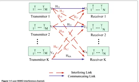
Desired signal power maximization IA model Consider a K-user interference MIMO channel (M × N,d)K as in Figure 1, where each transmitter equips with Mantennas, each receiver withNantennas and each user pair wishes to achievedDoFs. Supposesk ∈Cd×1denotes the transmit signal vector of the kth user with power covariance as E(sksHk) = (P/d)Id, whereP is the total transmit power of each user. For convenience we unify the transmit power of each stream, i.e.P/d=1. After receiv-ing the signal yk, the kth receiver multiplies decoding matrix to it on the left, which is expressed as:
UHkyk =UHkHkkVksk
desired signal
+
l=k,l∈K
UHkHklVlsl
interference
+UHknk
noise
,
(1)
whereHkl ∈ CN×M denotes the channel matrix between thekth transmitter and thelth receiver, andVk ∈CM×d,
Uk∈CN×drepresent the precoder and decoder of thekth
user, respectively. The three terms of (1) on the right side represent the desired signal, the interference from other users and the noise with distribution ofCN(0,σk2IN)at thekth receiver, respectively. In this article we assume all the noises have the same covariance, that is σk2 = σ2, k∈K.
Following the feasible condition for IA system, IA scheme is defined as[7]:
UHkHklVl=0,k=l,k,l∈K; (2)
rank(UHkHkkVk)=d,k∈K; (3)
VHkVk=Id,UkHUk =Id,k∈K. (4)
The original idea of IA only consists of (2) and (3). Noticing that for any precoding and decoding matri-ces {Vk,Uk,k ∈ K} that satisfy these two conditions, {VkPk,UkQk,k ∈ K} also satisfy (2) and (3) as long as {Pk,Qk ∈ Cd×d,k ∈ K} are all non-singular matrices. This indicates that the solutions of the IA system are not unique and the solution matrices formd-dimensional sub-spaces. Therefore, we require the columns ofVk,Uk,k ∈ K to be the orthogonal basis of the corresponding sub-spaces, which is the condition (4).
Besides the requirement of (2) and (4), we wish to maximize the desired signal power, in order to achieve suf-ficiently high sum rate. Suppose all the transmit signals are
statistically independent of each other. We can obtain the expected total desired signal power
PS= k∈K
Es(UHkHkkVksk22)=
k∈K
UHkHkkVk2F.
Based on the above analysis, we present the desired signal power maximization (PM) model as follows:
max Uk,Vk k∈K
PS(Uk,Vk)=
k∈K
UHkHkkVk2F (5a)
s. t. UHkHklVl =0, k=l,k,l∈K, (5b)
VHkVk =Id,UkHUk =Id, k∈K. (5c)
This model was first brought in [11], in which its per-formance is compared with the sum rate maximization (SRM) model. The PM model can achieve similar perfor-mance as the SRM model, while its related optimization problem is much simpler. Therefore it is a good way to approximate the SRM model by the PM model [11]. Thus in this article we only focus on solving (5) to design proper precoders and decoders.
The sum of squares of the residuals of constraints (5b) is the total leakage interference, which is given by:
PI(Uk,Vk)=
k∈K
Es ⎛ ⎜ ⎝ l=k,l∈K
UHkHklVlsl
2⎞
⎟ ⎠
=
k∈K
l=k,l∈K
UHkHklVl2F.
(6)
The essential idea of the AMA given by [7] is to mini-mizePIalternately forUk andVk. From the formulation of (5), we know that the MSP algorithm in [11] solves it by increasing PS while reducingPI towards zero at the same time. Here we briefly introduce the framework of MSP. In each iteration for each precoder and decoder, an AMA step is first taken to reduce PI. And then the iterative point go along the gradient direction of PS to increase it, whose stepsize gradually shrinks to 0 in order to perfectly align the interference by simply taking AMA steps in the last few iterations. MSP algorithm requires a series of eigenvalue decompositions and SVDs, which bring in high computational complexity and complicated matrix computations. Therefore we wish to propose algo-rithms for (5) with lower complexity and less complicated computations.
Modified alternating minimization algorithm (MAMA)
In this section, we present our first low complexity algo-rithm, the MAMA. The main difficulty for solving the highly nonlinear nonconvex optimization problem (5) is to deal with the nonlinear constraint (5b). Noticing that
(5a) and the penalty term (6) for (5b) have quite simi-lar expressions, we can combine these two together by the Courant penalty function technique [12] as in the next section.
Courant penalty function technique
Courant penalty function technique is a classic penalty function technique, which avoids dealing with constraints by moving them to the objective function. The basic idea is to replace the constraints with a penalty term scaled by a parameterC. The penalty term is the sum of squares of all the constraint violations. In (5), we apply Courant penalty technique to (5b) and keep the constraints (5c) in order to obtain the following simple constrained problem:
min Uk,Vk k∈K
P(Uk,Vk,C)=CPI(Uk,Vk)−PS(Uk,Vk)
(7a)
s. t. VHkVk=Id,UHkUk=Id, k∈K, (7b)
wherePIis defined by (6).
It is well known that if (5) is feasible, the solution of (7) converges to that of (5) asCapproaches infinity[13]. Thus the solution of (5) can be approximated by that of (7). As pointed out in [13], the approximated error between the solutions of (7) and (5) is of the level O(C1), which concerns about the choice of the penalty parameter C. Therefore, theoretically, (7) with largerCwould get bet-ter approximation of (5). However, in real computations, largeCmay lead to ill-conditioned objective function and consequently bring in numerical calculation difficulties. To avoid such difficulties caused by unnecessarily largeC in the first few iterations, we initially setCas a small pos-itive number such as C = 1. If sufficient reduction in PI is not achieved, we increaseC toσ
0C, whereσ0 > 1
is a constant. The solution of (7),(Uk(C),Vk(C),k ∈ K) provides a good initial point for solving (7) again when C is replaced byσ0C. In this way we forcePI to reduce
towards 0 eventually and the optimal solution of (5) can be obtained.
The overall algorithm
Via Courant penalty function technique our main task is now how to solve (7), which is quite similar to the LIM problem in whichPIis to be minimized. We can rewrite (7) as:
min
Uk,Vk k∈K
P(Uk,Vk,C) (8a)
=
k∈K
tr
⎛ ⎝UHk
⎛ ⎝C
l=k,l∈K
HklVlVHl HHkl−HkkVkVHkHHkk ⎞ ⎠Uk
⎞ ⎠
=
k∈K
tr
⎛ ⎝VH
k ⎛ ⎝C
l=k,l∈K HH
lkUlUHl Hlk−HHkkUkUHkHkk ⎞ ⎠Vk
⎞ ⎠
The only difference between the LIM problem and (8) is the objective function, as LIM minimizes the total leakage interferencePIsubject to (8b). Thus, we can borrow the idea of the AMA in [7], to iterateVk,k∈KandUk,k∈K alternatively in each iteration. Fixing allVk,k ∈Kin (8),
Uk,k∈Kbecome independent of each other. In this case, (8) turns intoKindependent subproblems with formulas as:
min
Uk
tr
⎛ ⎝UHk
⎛
⎝C
l=k,l∈K
HklVlVHl HHkl−HkkVkVHkHHkk ⎞ ⎠Uk
⎞ ⎠
s. t. UHkUk=Id.
(9)
We can obtain the closed-form solution of (9) asUk = νmind (Jk),k ∈ K, which means the columns of Uk are eigenvectors corresponding to thedsmallest eigenvalues of
Jk=C
l=k
HklVlVHl HHkl−HkkVkVHkHHkk.
Similar solutions ofVk can be achieved when fixing all
Uk,k ∈ K. Of course, we need a technique to update the penalty parameterCaccording toPIduring iterations.
Based on the above descriptions, our MAMA for the PM model (5) is stated as follows (Algorithm 1).
Algorithm 1: modified alternating minimization algorithm
1. Set initial precodersVkand decodersUk,k∈K, the
initial penalty parameterC andσ0>1.
¯
PI=PI(U k,Vk).
2. For decoders:Uk=νmind (Jk),k∈Kfrom above.
3. For precoders:Vk=νmind (˜Jk),k∈K, where ˜
Jk =Cl=kHHlkUlUlHHlk−HHkkUkUHkHkk.
4. If the algorithm converges, then stop and output Vk,Uk,k∈K. IfPI(Uk,Vk) >P¯I−1/C, then
increase the penalty parameterC:=σ0C. If
PI(Uk,Vk) <P¯I, letP¯I=PI(Uk,Vk). Go to step 2.
In the original AMA of [7], eigenvectors correspond-ing to thedsmallest eigenvalues of positive semi-definite matrices {l=kHklVlVHl HHkl,k ∈ K} and those of {l=kHHklUlUHl Hkl,k∈ K}are required. In our MAMA, the matricesJk and˜Jk are not necessarily positive semi-definite, since the objective function value of (8) might be negative with feasible solution of quite lowPIand highPS. Although our MAMA avoids calculating SVD which is required by the MSP algorithm given by [11], eigenvalue decompositions are still required for solving subproblems. This lends an impetus to further improvement.
A hybrid algorithm
In order to further reduce the complexity of our MAMA, we propose a hybrid technique in this section. First, we give an AHT, which is a very low complexity algorithm for (5). This algorithm is free from complicated matrix com-putation, such as eigenvalue decomposition, SVD and QR factorization, and enjoys lower computational complexity than MAMA.
Algorithm with Householder transformation
In this algorithm, we still use the Courant penalty function technique. Thus we focus on problem (7). The only con-straints of (7) are orthogonal concon-straints. We require all the iterative pointsUkandVkgenerated by our algorithms are feasible, namely (7b) are always satisfied. By requir-ing feasibility, basically we are solvrequir-ing an unconstrained optimization problem on the Grassmann manifold. Oth-erwise, if we allow iterations go outside the feasible region, we will have to adopt some technique, such as projec-tion, to draw the iterations back to the feasible region, which can be complicated. For example, the projection to the set of orthogonal matrices can be a non-differentiable operator and time-consuming to compute.
Preserving orthogonality
LetVikdenotes the precoder of thekth user in theith iter-ation. Suppose both Vik andVik+1 are orthogonal, there should exist a unitary matrixPik∈CM×Msuch that
PikVik =Vik+1.
The straightforward approach is to search for all uni-tary matrices Pik ∈ CM×M, but this can be computa-tionally very expensive. We consider a special class of unitary matrices, the Householder matrices, which can be represented as P = I− 2ppH with pHp = 1. The use of Householder transformation can not only preserve orthogonality, but also turn the problem from a matrix optimization into a vector optimization problem. In the ith iteration with fixed Vik,Uik,k ∈ K as certain feasi-ble solution of (7), we try to obtain orthogonal vectors vk,uk,k∈Kand set
Vki+1=(IM−2vkvHk)Vik,Uki+1=(IN−2ukuHk)Uik, k∈K
(10)
as the precoders and decoders in the(i+1)th iteration. Here,vk,uk,k ∈ K are regarded as optimal (or subopti-mal) solutions to minimize the objective function value of (7), P(Uik+1,Vik+1,C) = P((IN − 2ukuHk)Uik,(IM − 2vkvHk)Vik,C).
Alternating directions
Substituting (10) into (7), we get (11) with variables
vk,uk,k∈K:
min
uk,vk k∈K
k∈K ⎛ ⎝C
l=k,l∈K
(Uil+1)HHlkVik+12
F− (Uik+1) HHkkVi+1
k 2 F ⎞ ⎠
=
k∈K ⎛ ⎝C
l=k
(Uil)H(IN−2uluHl )Hlk(IM−2vkvHk)Vik2F
−(Uik)H(IN−2ukuHk)Hkk(IM−2vkvHk)Vik2 F ⎞ ⎠
s. t.vHkvk=1,uHkuk=1, k∈K.
(11)
With the fact that
(Uil+1)HHlk(IM−2vkvHk)Vik2F = tr(Vik)H(IM−2vkvHk)HHlkUli+1(Uil+1)
HH
lk(IM−2vkvHk)Vik
= 4tr(Vik)HvkvHkHHlkUil+1(U i+1
l )HHlkvkvHkVik
−2tr(Vik)HvkvHkHHlkUil+1(U i+1
l )HHlkVik +(Vik)HHHlkUil+1(Uil+1)HHlkvkvHkVik
+tr(Vik)HHHlkUli+1(Uil+1)HHlkVik
= 4(vHkHHlkUli+1(Uil+1)HHlkvk)(vHkVki(Vik)Hvk) −2(vHkHHlkUil+1(Uli+1)HHlkVik(Vik)Hvk +vHkVik(Vki)HHHlkUli+1(Uil+1)HHlkvk) +tr(Vik)HHHlkUli+1(Uil+1)HHlkVik
,
(12)
we can rewrite the objective function of (11) as:
k∈K
4(vHkAkvk)
vHkVik(Vik)Hvk
−2vHkAkVik(Vik)Hvk+vHkVik(Vik)HAkvk
+tr(Vik)HAkVik
,
(13)
where Ak = Cl=k,l∈KHHlkU i+1
l (U i+1
l )HHlk −
HkkHUik+1(Uki+1)HHkk,k∈K.
Fixing allul,l ∈ Kin (11),Uli+1,l ∈ Kare determined according to (10), and thusvk,k ∈ K become indepen-dent of each other. Therefore, (11) is decomposed intoK subproblems with the same form as follows:
min
x∈CM f(x)=(x
HAx)(xHBx)−xHCx
s. t. xHx=1. (14)
Here x represents vk. A = 2
Cl=k,l∈KHHlkUil+1 (Uil+1)HHlk−HHkkUik+1(Uik+1)HHkk
,B=2Vik(Vik)Hand C=(AB+BA)/2. Similarly, fixing allvk,k∈K, it yields K subproblems like (14) from (11). Based on the analysis
above, the alternating direction method can be applied to optimizevk,k∈Kanduk,k∈Kalternatively.
Subproblem: 2D subspace method
Subproblem (14) is a nonlinear optimization on the Stiefel manifold in complex field, which is not easy to han-dle. With the aim of low complexity, we abandon the second order method where Hessian matrix information is required. Instead, we apply a 2D subspace method to solve it iteratively [14]. We define the subspace spanned byx0andg˜as
S(x0,g˜)=
x:x=bx0+ag˜.a∈[−1, 1] ,b=
1−a2,
wherex0is the current iterative feasible point andg˜
repre-sents its normalized gradient of the Lagrangian function of (14). In each step, the feasible domain ofxshrinks from the Stiefel manifoldxHx=1 toS(x0,g˜).
Here g˜ is calculated as follows. First, the Lagrangian function of (14) is expressed as:
L(x,λ)=f(x)−λ(xHx−1), (15)
whereλis the Lagrange multiplier. Then the gradient of (15) is
g=g0−λx0, (16)
whereg0is the gradient of the objective functionf at the
pointx0:
g0=2[(xH0Ax0)Bx0+(xH0Bx0)Ax0−Cx0] .
As a necessary condition of the first order optimal-ity condition of (14), we require gHx0 = 0. Thusλ =
2(xH0Ax0)(xH0Bx0)−xH0Cx0is deduced due toxH0x0=1.
Onceλis computed,gcan be chosen by (16) and we can letg˜ =g/g2.
To maintainS(x0,g˜) on the Stiefel manifold, any point x∈S(x0,g˜)should satisfyxHx=b2x02+a2˜g2=1.
Thusa2+b2 = 1,a ∈[−1, 1], namelyb = ±√1−a2.
For anya∈[−1, 1], the objective function of (14) share the same function value at√1−a2x
0+ag˜and−
√ 1−a2x
0−
ag˜. Therefore, we only consider the caseb = √1−a2to
avoid redundant solutions.
Taking the expression ofx∈ S(x0,g˜)into (14), it turns
into a one dimensional constraint optimization problem with variablea:
min a∈[−1,1]p1a
1−a2+p2a2+p 3a3
1−a2+p4a4, (17)
where the current iterative pointx0corresponds toa=0,
and
p1=2[ Re(xH0Ag˜)(xH0Bx0)+Re(xH0Bg˜)(xH0Ax0)−Re(xH0Cg˜)] ,
p2=(xH0Ax0)(g˜HBg˜)+(xH0Bx0)(g˜HAg˜)−2(xH0Ax0)(xH0Bx0) +4Re(xH
0Ag˜)Re(xH0Bg˜)+xH0Cx0− ˜gHCg˜,
p3=2[ Re(xH0Bg˜)(g˜HAg˜−xH0Ax0)+Re(xH0Ag˜)(g˜HBg˜−xH0Bx0)] ,
Newton’s method with line search is applied to solve (17) and a local minimizer is guaranteed to be found [13]. The method to solve subproblem (14) is summarized as follows:
Subalgorithm: two dimensional subspace method
1. Given any initial feasible pointx0and the maximum iteration numberTinner,t1=1.
2. Calculateg˜and construct subproblem (17).
3. Solve (17) by Newton’s method with line search and
x0:=
√ 1−a2x
0+ag. If the objective function of˜
(14) does not reduce ort1=Tinner, stop and output x0; elset1:=t1+1, go to Step 2.
The maximum iteration number Tinner relates to the efficiency of the algorithm. It should not be too large or too small, in order to avoid spending too much time for subproblem or insufficient reduction of the objec-tive function value. We will discuss its specific choice in Section “Simulations”.
As the projection to the Stiefel manifoldxHx=1 is very easy to compute, projected gradient method is also a com-mon approach to solve (14). In the following theorem and remark, we compare our 2D subspace method with the projected gradient method and show the advantage of our method.
Theorem 1. Denote the projected gradient step started
fromx0with stepsizeαas:
x(α)= x0−αg0
x0−αg0
. (18)
On one hand, for any vectorx ∈ S(x0,g˜), there exists a
stepsizeα∈R, such thatxis expressed as (18); on the other hand, for anyα ∈ R, the projected gradient stepx(α)can be expressed as the linear combination ofx0andg˜, which
meansx(α)∈S(x0,g˜).
Proof. See the Appendix.
Remark 1. Theorem 1 shows that step in certain 2D
sub-space and the projected gradient step can be mutually expressed. Thus the minimization of the objective function f on the 2D subspace S(x0,g˜)and that along the projected
gradient step are essentially the same. The 2D subspace problem is easy to handle, as shown above; but the search for (18) may be quite difficult, because the projection oper-ator would make the objective function nondifferentiable and lose the common Taylor expansion, consequently it is nontrivial to search for proper stepsizeα. Due to these con-siderations, we use the 2D subspace method rather than the projected gradient method to solve (14).
Framework of AHT algorithm
According to the above discussions, the framework of the AHT algorithm can be concluded as follows (Algorithm 2).
Algorithm 2: algorithm with Householder transformation
1. Set initial precoders and decoders asV0k,U0k,k∈K, parameterTinnerin 2D subspace, the maximum
inner iteration numberTouter, the initial penalty
parameterC, parameterσ0>1forC and the stopping parameterε.i=0.
2. Solve (11) iteratively: fixUik,Vik,k∈K, and set the initial normalized vectorsuk,vk,k∈K.t=1.
(2.1) For precoders: fixuk,k∈K. Fork∈K,
constructA,B,Cin (14) and solve it with 2D subspace method to obtainvk.
(2.2) For decoders: fixvk,k∈K. Similarly to Step
2.1, obtain newuk,k∈Kby solving (14).
(2.3) CalculateUik+1,Vki+1,k∈Kfrom (10). If
t=Touteror
PI(Uik+1,Vik+1)≤PI(Uik,Vik)−1/C, go to Step 3; elset:=t+1, go to step 2.1.
3. IfPI(Ui+1
k ,Vik+1) >PI(Uik,Vik)−1/C, increase the
penalty parameterC:=σ0C. IfPI(Uki+1,Vik+1) < ε, stop and outputUk :=Uik+1,Vk:=Vik+1,k∈K; else i:=i+1, go to Step 2.
In our simulations,t is usually no more than 5 when PI(Uik+1,Vik+1) ≤ PI(Uik,Vik)− 1/C is achieved in Step 2.Touter, the maximum number of inner iterations inside Step 2, acts to avoid extreme situation with too much time to solve subproblems. Thus we suggestTouter=5.
Hybrid algorithm
Although the AHT algorithm enjoys lower complexity than MAMA as analyzed in the next section, it solves subproblem (14) inexactly by successive 2D subspace minimizations. This reduces the objective function value rapidly at first, however the speed becomes much more slowly when the iterative point approaches a local optimal solution. Simulation also verifies that it is quite difficult to align the interference perfectly with the AHT algorithm. In contrast, MAMA solves subproblem (9) exactly with closed form solution. The sequence generated by MAMA converges fast near the solution, which is complementary to that of AHT.
In order to make full use of the low complexity of AHT and the fast local convergence property of MAMA, it seems reasonable for us to combine these two methods together into a hybrid algorithm. We believe that such a hybrid algorithm will enjoy the properties of low complex-ity and fast local convergence, which are verified by our simulation tests reported in Section “Simulations”.
to converge to the solution, by starting from the point obtained by AHT (Algorithm 3).
Algorithm 3: hybrid algorithm
1. Set initial precoders and decoders asV0k,U0k,k∈K, the penalty parameterC=1.
2. Input the initial iterative point and penalty parameter into the AHT algorithm. Set its stopping criterion as
PI(Uk,Vk) <0.01PI(U0k,V0k). Output the
correspondingVk,Uk,k∈Kand the current penalty
parameterCAHT=C.
3. InputVk,Uk,k∈KandC=CAHTas the initial iterative point and penalty parameter of MAMA, respectively. Iterate until convergence by the MAMA. Output the corresponding precoders and decodersVk,Uk,k∈K.
In some sense, it can be viewed that the AHT algorithm acts as a method to rapidly find a good initial point with low interference for MAMA. Starting from the good initial point, MAMA can converge very fast to a local optimal solution with perfect IA.
Analysis of computational complexity
In this section, we analyze the computational complexity of IA algorithms for PM model, including our two pro-posed algorithms MAMA and AHT, as well as the MSP algorithm from [11].
Advantages of low complexity algorithms
Before presenting the detailed analysis on the computa-tional complexities of different algorithms, we provide the reasons for constructing low computational complexity IA algorithms for the PM model.
1. No matter our algorithms or the existed IA
algorithms, they all exploit the channel reciprocity to design the transmit precoders and receiver decoders in a distributed way. Such reciprocity is based on the time division duplex (TDD) operation with
synchronized time-slot in the practical system. However, due to the time varying property of wireless channel, perfect reciprocity may be hard to achieve and result in residual interference at the receivers. This requires algorithms with short computing time to reduce the possibility of performance loss due to the imperfect reciprocity in practical systems[15]. 2. Furthermore, that the receivers generally have
limited computational complexity, might be a bottleneck for the complexity of the algorithms. Thus we need to design algorithms with low complexity and simple computation, to satisfy the computation restriction of communication equipments.
3. Also, algorithms with lower complexity are easier to be extended to large scale problems. For small scale problems, algorithms with low or high complexity do not differ much from each other. However as the problem dimension grows, high complexity algorithms can be very very slow for large scale problems because of too much computing time, while algorithms with lower complexity are more preferable.
Detailed analysis
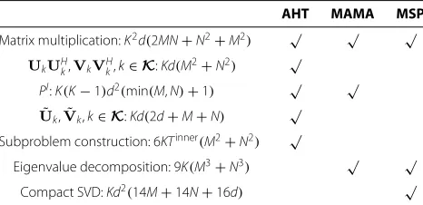
Here we consider the number of complex multiplica-tions as the complexity criterion. The AHT, MAMA and MSP algorithm are analyzed and compared. Their main computations in one iteration are listed as follows:
1. The computation ofHklVlVHl HHkland
HHlkUlUHl Hlk,k,l∈Kare required for all the three
algorithms. LetH˜kl =HklVl. Then we can calculate
HklVlVHl HklHasH˜klH˜Hkl. Similarly we can compute
HlkHUlUHl Hlkby introducingH¯lk =HHlkUl. Ask and l
traverse all the elements inK, the entire complexity isK2[(dMN+dN2)+(dMN+dM2)]=
K2d(2MN+N2+M2).
2. Besides term 1, the AHT algorithm requires to computeUkUHk andVkVHk, with complexity of Kd(M2+N2).
3. PIis computed in both the AHT and MAMA.
Noticing that
PI= k∈K
l=k,l∈K
UHkHklVl2F=
k∈K
l=k,l∈K
VHkHHlkUl2F,
we can computeUHkH˜kl2FifN<M, orVHkH¯lk2F
otherwise, whereH˜klandH¯lkare the pre-computed
parameters in term 1. With the above analysis, the corresponding complexity is
K(K−1)d2(min(M,N)+1).
4. AHT algorithm requires to update precoders and decoders by computingUik+1,Vki+1,k∈Kin (10). WithUik+1=Uik−2uk(uHkUik), the complexity is K[(d2+dM)+(d2+dN)]=Kd(2d+M+N). 5. In each inner iteration of our 2D subspace method
for (14) in the AHT algorithm, it mainly requires computation ofAx,Bx,Cx=[A(Bx)+B(Ax)]/2,
AgandBg, the complexity of which is6n2, wheren
is the dimension ofx. Suppose for each 2D subspace method, there are mostlyTinnerinner iterations, we can see that each iteration of AHT requires the total complexity of6KTinner(M2+N2).
with dimensionN×N. The entire complexity is 9K(M3+N3).
7. The complexity of one compact SVD of matrix with dimensionM×d(d<M) is14Md2+8d3[16]. The MSP algorithm requiresK compact SVDs for matrices with dimensionM×dandK with dimensionN×d, whose complexity is
Kd2(14M+14N+16d).
Table 1 shows the specific computational complexity of the three algorithms. Comparing the AHT and MAMA, besides the common terms, AHT owns term 2,4,5, while MAMA has term 6. With the fact that 1 ≤ d ≤ min(M,N), we can deduce that:
Kd(2d+M+N)+Kd(M2+N2) ≤2Kd(M+N)+Kd(M2+N2)
≤3K(M2+N2) <3K(M3+N3). (19)
For term 5, as long asTinner≤min(M,N), we have
6KTinner(M2+N2)≤6K(M3+N3). (20)
Adding both sides of (19) and (20), we conclude that AHT has lower complexity than MAMA.
Similarly, we compare term 3 and term 7 to see the dif-ference between the complexity of MAMA and MSP. As long as K ≤ 23 (which is usually the case in practical considered IA problems), the following inequality holds:
K(K−1)d2(min(M,N)+1)≤22Kd2(min(M,N)+1) ≤Kd2(22 min(M,N)+22d)≤Kd2(14M+14N+16d).
So the complexity of MAMA is lower than that of the MSP algorithm. Thus the algorithms ranked from low to high complexity in one iteration are AHT, MAMA and MSP. This also implies that the hybrid algorithm has lower complexity than MAMA and MSP.
Our above analysis compares the complexity of each iteration of different algorithms. However, in order to compare the computational complexity of different algo-rithms, we need to estimate the total number of iterations of all the algorithms under considerations, which is not
Table 1 Comparison of computational complexity
AHT MAMA MSP
Matrix multiplication:K2d(2MN+N2+M2) √ √ √
UkUHk,VkVHk,k∈K:Kd(M2+N2)
√
PI:K(K−1)d2(min(M,N)+1) √ √
˜
Uk,V˜k,k∈K:Kd(2d+M+N) √ Subproblem construction: 6KTinner(M2+N2) √
Eigenvalue decomposition: 9K(M3+N3) √ √
Compact SVD:Kd2(14M+14N+16d) √
easy. Therefore, we try to explain it by convergence curves with consuming time in simulations.
Simulations
In this section, we analyze our proposed algorithms the MAMA, AHT and hybrid algorithm by simulations, and compare them with the existed AMA [7] and MSP algo-rithm proposed in [11].(5×5, 2)4interference channels are considered, that is,K = 4,M=N =5,d =2, which satisfy the general feasibility condition [2,3]. Each compo-nent ofHkl,k,l∈Kis i.i.d complex Gaussian distribution CN(0, 1).
We use sum rate as the measure of quality of service. The sum rate of theK-user MIMO interference channel is expressed as follows:
R=
k∈K
logIN +F−k1Lkk
=
k∈K
logIN + ⎛ ⎝σ2IN+
l=k,l∈K
Lkl
⎞ ⎠
−1
Lkk
, (21)
where Lkl = HklVlVHl HHkl,k,l ∈ K, Fk = σ2IN +
l=k,l∈KLklandσ2is the covariance of the additive white Gaussian noise at the receivers. Here we define the SNR as SNR=P/σ2=d/σ2.
In the AHT algorithm, we set Touter = 5 and ini-tially C = 1. For each figure, 250 random realization of different channel coefficients are generated to evaluate the average performance. For each realization the initial values of precoders and decodersV0k,U0k,k ∈ K are ran-domly generated and remain the same in the compared algorithms.
Parameter analysis
As mentioned before, the choice ofTinner relates to the efficiency of the AHT algorithm and also the hybrid algo-rithm. In Figure 2 we plot the convergence curves of the hybrid algorithms with parameter Tinner = 3, 5, 10, respectively. SNR equals 30 dB andσ0=20 here.
Figure 2 reveals that, both the converged average sum rate and the convergence rate of the hybrid algorithms with different Tinner are quite similar. The curve with Tinner=10 seems to be the worst, which accords with our complexity analysis asTinner > min(M,N) = 5. In the upcoming simulations we setTinner = 5 with which the hybrid algorithm obtains the highest sum rate, to improve the efficiency of our proposed algorithms.
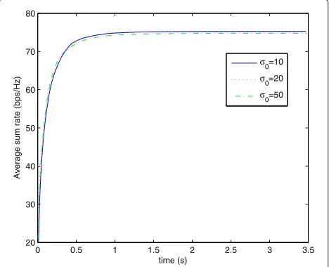
Besides Tinner, we also compare the performances of the hybrid algorithms with differentσ0.σ0determines the growth speed of the penalty parameter C, which repre-sents the weight ofPIin the objective function of (7). If σ0 is too small, it would take many iterations for C to
0 0.5 1 1.5 2 2.5 3 3.5 20
30 40 50 60 70 80
time (s)
Average sum rate (bps/Hz)
T
inner=5
T
inner=3
T
inner=10
Figure 2Convergence of the average sum rate of the hybrid algorithms withTinner=3, 5, 10.
algorithm. On the other side, too large σ0 forces C to
grow too fast, which makes (7) degenerate into the LIM problem in short time and that PS cannot be increased efficiently.
Based on the aforementioned analysis, we plot the con-vergence curves of the hybrid algorithms with σ0 = 10, 20, 50 in Figure 3. SNR is also set as 30 dB here. The three curves are very close to each other, which indicates that the algorithm is not sensitive toσ0. In the following
simulations we setσ0=20.
AHT algorithm
In this section, the relative iteration number to achieve certain leakage interference of the AHT and MSP algo-rithm are displayed in Figure 4, to show the property of
0 0.5 1 1.5 2 2.5 3 3.5
20 30 40 50 60 70 80
time (s)
Average sum rate (bps/Hz)
σ0=10
σ0=20
σ0=50
Figure 3Convergence of the average sum rate of the hybrid algorithms withσ0=10, 20, 50.
0 0.2 0.4 0.6 0.8 1
10−2 10−1 100 101
Normalized iteration number
Leakage interference
AHT MSP
Figure 4Comparison of AHT and MSP: total leakage interference versus normalized iteration number.
AHT algorithm. The stopping criterion is PI ≤ 0.01. The average number of iterations of the MSP and AHT algorithm to solve one problem are 1233 and 583, respec-tively. To analyze the relative convergence performance, we use the normalized iterations, the ratio of the itera-tions at the certain point and the total iteraitera-tions, as the x-axis. And they-axis represents the total leakage interfer-encePI. Figure 4 implies that to achieve the interference of 0.5 from the initial point, the AHT algorithm requires 7.5% of its total iterations while MSP requires 45%. Com-pared to the MSP algorithm, the AHT algorithm iterates rapidly to a point with low leakage interferencePI. Actu-ally the main consuming time of AHT algorithm is used to reducePIfrom less than 1 towards 0.01, and the conver-gence rate becomes much slower whenPIis smaller. The performances here accords with the previous analysis.
Comparison of different IA algorithms
In this section, the performances of different IA algorithms are compared and analyzed, including our pro-posed MAMA, AHT and hybrid algorithm, as well as the existed MSP and AMA. The number of iterations of each algorithm to solve each problem is set as 3000, in order to perfectly align the interference. To take full advantage of AHT, we set its stopping parameter ε = 0.01PI(U0k,V0k), whereV0k,U0k,k ∈ K are the initial pre-coders and depre-coders.
0 5 10 15 20 25 30 35 40 10
20 30 40 50 60 70 80 90 100
SNR (dB)
Average sum rate (bps/Hz)
MSP Hybrid MAMA AMA
Figure 5Comparison of MAMA, Hybrid, MSP and AMA: average sum rate versus SNR.
are quite close to each other. The solutions of the three algorithms are quite different, whereas they get similar sum rate under the same SNR. And all the three algo-rithms gain about 5 bps/Hz higher sum rate than the AMA under medium and high SNR. In Figure 6, both of our pro-posed two algorithms require much less computing time than the MSP algorithm. Particularly, the hybrid algo-rithm gain almost as high sum rate as MSP with as little time as the AMA.
To further compare the convergence performances of these four algorithms as well as AHT algorithm, we plot their convergence curves of sum rate with respect to the running time in Figure 7. As AHT algorithm is difficult to converge and eliminate interference, it is shown as the first
0 5 10 15 20 25 30 35 40 0.8
1 1.2 1.4 1.6 1.8 2
SNR (dB)
Relative computing time
MSP Hybrid MAMA AMA
Figure 6Comparison of MAMA, Hybrid, MSP and AMA: average relative computing time versus SNR.Time of AMA is set as standard.
0 1 2 3 4 5
10 20 30 40 50 60 70 80
time (s)
Average sum rate (bps/Hz)
MSP AHT Hybrid MAMA AMA SNR=30dB
SNR=15dB
SNR=5dB
Figure 7Convergence of the average sum rate of MAMA, AHT, Hybrid, MSP and AMA with respect to SNR = 5, 15, 30 dB.
stage of the hybrid algorithm. Its output point is used to continue iteration in the hybrid algorithm. SNR are set as 5, 15 and 30 dB to represent the scenarios of low, medium and high SNR, respectively. In all three scenarios, both MAMA and the hybrid algorithm achieve similar con-verged average sum rate as the MSP algorithm, which gain more sum rate than the AMA. To achieve a certain sum rate, MAMA consumes the least time. We also observe an interesting phenomenon, that in the low and medium SNR scenario each of the MAMA, hybrid and MSP algorithm achieves high sum rate during iteration before conver-gence, after that it reduces and converges to a lower rate. This may be relevant to the value ofσ2. As shown at the beginning of this section, SNR value is inversely propor-tional toσ2. For the low SNR scenario,σ2is considerably high and σ2IN takes the main part ofFk in (21). Then, the sum rate mainly increases with largePS. All the three concerned algorithms are designed to increasePSin the first few iterations and gradually reduce the weight of this requirement. This may lead to the phenomenon thatPS increases to a peak value and then decreases gradually, which explains the similar phenomenon of sum rate in Figure 7.
0 1 2 3 4 5 10−5
10−4 10−3 10−2 10−1 100 101 102
time (s)
Leakage interference
MSP AHT Hybrid MAMA AMA
Figure 8Convergence of the leakage interference of MAMA, AHT, Hybrid, MSP and AMA with respect to SNR = 30 dB.
Comparing the proposed MAMA and hybrid algorithm from both aspects of computing time and convergence rate in Figures 6, 7 and 8, we should admit that the improvement of the hybrid algorithm over MAMA is lim-ited in the examples that we tested. The main reason of this phenomenon is due to the quite small scale of the test problems, for which lower complexity algorithm does not have much gain. Nevertheless, as the dimension of the problem increases, the hybrid algorithm will save more consuming time and benefit more. Moreover, in similar applications in other fields, there might be large scale sim-ilar matrix optimization problems, we believe that the hybrid algorithm will improve MAMA greatly.
Remark 2. We have pointed out in Section “A hybrid
algo-rithm” that the sequence generated by the hybrid algorithm converges to a local optimal solution. Although it is not guaranteed to be global optimal, the obtained local opti-mal solution performs with high sum rate (almost the same as MSP algorithm and higher than the AMA, as depicted in Figure 5) and perfect IA. Such solution satisfies our requirement for an IA solution.
The performances of MAMA and the hybrid algorithm in this section indicates that the Courant penalty function technique is an effective way to combine the leakage inter-ference and the desired signal power together. Through this technique, both algorithms achieve high average sum rate in short time. In the last few iterations when C becomes very large, the algorithm essentially tries to minimize PI with the part of −PS being nearly ignored. Therefore, MAMA (also the hybrid algorithm) eventually behaves very similar to the original AMA, which can perfectly align the interference.
Conclusion
This article proposed two low complexity algorithms for the desired signal power maximization IA problems of MIMO channels. The IA constraints are added to the objective function and combined with the desired signal power via the Courant penalty function technique. First, a MAMA is proposed following the similar approach of the AMA. Then, a hybrid algorithm is proposed to fur-ther reduce complexity. In the hybrid algorithm, the AHT is proposed to iterate rapidly from any initial point to pre-coders and depre-coders with low leakage interference. This step provides a good point around the local optimal solu-tion. From this point, MAMA is applied to converge fast to the local optimal solution satisfying our requirement. Analysis shows that, among the compared algorithms the hybrid algorithm has the lowest computational complex-ity, followed by MAMA, with MSP being the highest. Simulations indicate that both the hybrid algorithm and MAMA achieve similar sum rate as the MSP algorithm with less computing time, and higher sum rate than the AMA.
Appendix Proof of Theorem 1
As stated in (16),g0is the linear combination ofx0andg˜.
Suppose
g0=c1x0+c2g˜,
wherec1andc2are scalars.
First prove that the projected gradient step can be expressed by 2D subspace step. For the projected gradi-ent step x(α) with any α ∈ R, we would like to find corresponding scalarsaandb, such that
x(α)= x0−αg0
x0−αg0 =
(1−c1α)x0−c2αg˜
(1−c1α)x0−c2αg˜ =
bx0+ag˜.
(22)
Let the coefficients ofx0andg˜remain unchanged, then
a= −c2α
(1−c1α)x0−c2αg˜
,b= 1−c1α (1−c1α)x0−c2αg˜
.
Next show that 2D subspace step can also be expressed by the projected gradient step. For any x ∈ S(x0,g˜), we
havex= bx0+ag˜. As we wish to findα ∈ Rsuch that x= x(α), then (22) holds. Similar to the proof above, we can induce that
b a =
c1α−1
c2α
,α= a
c1a−c2b
.
Competing interests
The authors declare that they have no competing interests.
Acknowledgements
The authors would like to thank the editor and two anonymous referees for their comments and suggestions which improved the article greatly. This work was partly supported by the National Natural Science Foundation of China (NSFC) grants 10831006, 11021101, by CAS grant kjcx-yw-s7 and by the Fundamental Research Funds for the Central Universities.
Author details
1State Key Laboratory of Scientific and Engineering Computing, ICMSEC,
AMSS, Chinese Academy of Sciences, Beijing, 100190, China.2Wireless Signal
Processing and Network Lab, Beijing University of Posts and Telecommunications, Beijing, 100876, China.
Received: 1 December 2011 Accepted: 14 June 2012 Published: 11 July 2012
References
1. VR Cadambe, SA Jafar, Interference alignment and degrees of freedom of theK-user interference channel. IEEE Trans. Inf. Theory.54(8), 3425–3441 (2008)
2. CM Yetis, T Gou, SA Jafar, AH Kayran, On feasibility of interference alignment in MIMO interference networks. IEEE Trans. Signal Process.
58(9), 4771–4782 (2010)
3. M Razaviyayn, G Lyubeznik, ZQ Luo, On the degrees of freedom achievable through interference alignment in a MIMO interference channel. IEEE Trans. Signal Process.60(2), 812–821 (2012) 4. SW Choi, S-Y Chung, On the multiplexing gain ofK-user partially
connected interference channel, preprint, http://arxiv.org/pdf/0806.4737. Jun 2008
5. M Guillaud, D Gesbert, Interference alignment in the partially connected K-user MIMO interference channel. inEuropean Signal Processing
Conference (EUSIPCO)(Barcelona, Spain, 2011), pp. 1095–1099
6. N Lee, D Park, Y-D Kim, Degrees of freedom on theK-user MIMO interference channel with constant channel coefficients for downlink communications. inProc. IEEE Global Telecommun. Conf., (GLOBECOM) (Hawaii, USA, 2009), pp. 1–6
7. K Gomadam, VR Cadambe, SA Jafar, A distributed numerical approach to interference alignment and applications to wireless interference networks. IEEE Trans. Inf. Theory.57(6), 3309–3322 (2011) 8. YF Liu, YH Dai, ZQ Luo, On the complexity of leakage interference
minimization for interference alignment. inIEEE Int. Workshop Signal
Process. Advances Wireless Comm(San francisco, USA, 2011), pp. 471–475
9. DA Schmidt, W Utschick, ML Honig, Large system performance of interference alignment in single-beam MIMO networks. inProc. IEEE
Global Telecommun. Conf., (GLOBECOM)(Miami, USA, 2010), pp. 1–6
10. H Shen, B Li, MX Tao, XD Wang, MSE-based transceiver designs for the MIMO interference channel. IEEE Trans. Wirel. Commun.9(11), 3480–3489 (2010)
11. I Santamaria, O Gonzalez, RW Heath Jr, SW Peters, Maximum sum-rate interference alignment algorithms for MIMO channels. inProc. IEEE Global
Telecommun. Conf., (GLOBECOM)(Miami, USA, 2010), pp. 1–6
12. J Nocedal, SJ Wright,Numerical Optimization(Springer, Berlin, 1999), pp. 488–522
13. YX Yuan,Computational Mehthod for Nonlinear Optimization (in Chinese) (Science Press, Beijing, 2008), pp. 16–20; 158–162
14. YX Yuan. inSome Topics in Industrial and Applied Mathematics (Series in
Contemporary Applied Mathematics CAM 8), ed. by Jeltsch R, Li DQ, and
Sloan IH. (Higher Education Press, Beijing, 2007), pp. 206–218
15. HG Ghauch, CB Papadias, Interference alignment: a one-sided approach.
inProc. IEEE Global Telecommun. Conf., (GLOBECOM)(Houston, USA, 2011),
pp. 1–6
16. GH Golub, CF Van Loan,Matrix Computations,3rd edn. (The Johns Hopkins University Press, London, 1996), pp. 248–255; 414–425
doi:10.1186/1687-6180-2012-137
Cite this article as:Sunet al.:Low complexity interference alignment algo-rithms for desired signal power maximization problem of MIMO channels. EURASIP Journal on Advances in Signal Processing20122012:137.
Submit your manuscript to a
journal and benefi t from:
7Convenient online submission 7Rigorous peer review
7Immediate publication on acceptance 7Open access: articles freely available online 7High visibility within the fi eld
7Retaining the copyright to your article