Nonlinear filtering based on 3D wavelet transform for MRI denoising

(1)

R E S E A R C H

Open Access

Nonlinear filtering based on 3D wavelet

transform for MRI denoising

Yang Wang

1*

, Xiaoqian Che

2

and Siliang Ma

1

Abstract

Magnetic resonance (MR) images are normally corrupted by random noise which makes the automatic feature extraction and analysis of clinical data complicated. Therefore, denoising methods have traditionally been applied to improve MR image quality. In this study, we proposed a 3D extension of the wavelet transform (WT)-based bilateral filtering for Rician noise removal. Due to delineating capability of wavelet, 3D WT was employed to provide effective representation of the noisy coefficients. Bilateral filtering of the approximation coefficients in a modified neighborhood improved the denoising efficiency and effectively preserved the relevant edge features. Meanwhile, the detailed subbands were processed with an enhanced NeighShrink thresholding algorithm. Validation was performed on both simulated and real clinical data. Using the peak signal-to-noise ratio (PSNR) to quantify the amount of noise of the MR images, we have achieved an average PSNR enhancement of 1.32 times with simulated data. The quantitative and the qualitative measures used as the quality metrics demonstrated the ability of the proposed method for noise cancellation.

Keywords:magnetic resonance imaging, 3D image denoising, 3D wavelet transform, bilateral filtering, enhanced NeighShrink thresholding

1. Introduction

Three-dimensional magnetic resonance imaging (MRI) has, during the last several decades, benefited from a variety of technological developments resulting in increased resolution, signal-to-noise ratio (SNR), and acquisition speed. However, fundamental trade-offs among resolution, acquisition speed, and SNR combined with scientific, clinical, and financial pressures to obtain more data more quickly, can result in images that exhi-bit significant artifacts, e.g., noise, partial volume, and intensity nonuniformity. For instance, the need for shorter acquisition times for patients in certain clinical studies often undermines the ability to obtain images having both high-resolution and high SNR. Another example concerns diffusion-tensor (DT) MRI that has become quite popular over the last decade due to its ability to measure the anisotropic diffusion of water in structured biological tissue. DT MRI differentiates between the anatomical structures of cerebral white

matter, which was previously impossible with MRI,in vivo, and noninvasively. The effects of Rician noise on DT MRI, however, are severe because of the inherent nature of the process–higher tissue anisotropy produces progressively lower intensities in diffusion-weighted images that, in turn, are more susceptible to Rician noise. The efficacy of higher-level post processing of MR and DT-MR images, e.g., segmentation and registra-tion, that assume specific models on regions of interests, e.g., homogeneous, is sometimes impaired by even mod-erate noise levels. Hence, it is necessary to remove the noise from MR image.

The removal of noise from noisy data to obtain the unknown signal is often referred to as denoising. Post-processing filtering techniques with the advantage of not to increase the acquisition time have extensively been used in MRI denoising. Many image denoising methods have been proposed in previous research. The conven-tional approach [1,2] was proposed to estimate the Rician noise level and perform signal reconstruction using a maximum likelihood method. Anisotropic diffu-sion [3-5] reduces image noise by considering a scale space, and it has been adapted to suppress the Rician * Correspondence: [email protected]

1

Department of Computational Mathematics, Jilin University, Chang chun, China

Full list of author information is available at the end of the article

(2)

noise in MR image [6]. Moreover, anisotropic diffusion filter combined with the Wiener filter [7] has been used for MRI denoising, which spatially averages pixels according to their correlation structure. The nonlocal means filter has been applied for feature preserved MRI denoising [8-12]. It builds an estimation of the restored pixel value by weighted averaging over a large portion of the pixels within the image. The weights are based on the similarity computed by comparing the patches instead of single point, and the edges and the details can both be well preserved.

Recently, wavelets have become a popular tool in various applications for data analysis and image pro-cessing. Application of wavelets for denoising of MR images has produced a large number of algorithms [13,14]. Early study [15] was followed by multi-scale products thresholding [16], which uses adjacent wave-let subbands to detach the edges from noise. Complex denoising of MR images using wavelets was proposed by Zaroubi and Goelman [17]. The method produces better SNR compared to the magnitude denoising scheme. Wu et al. [18] proposed a wavelet-based back-ground noise removal method in MRI. The proposed method can be used jointly with existing denoising methods to improve their effectiveness. Bilateral filter-ing in wavelet domain has been shown to preserve the edges efficiently [19]. Moreover, wavelet has been used for MRI denoising in combination with Radon trans-form, which estimates noise variance in different scales [20].

In this study, we proposed a 3D extension of the wavelet transform (WT)-based bilateral filtering ideas for Rician noise removal. Due to delineating capability of wavelet, 3D WT was employed to decompose the MR image into the approximation and the detailed sub-bands. Next, bilateral filtering of the approximate coeffi-cients in a modified 3D neighborhood improved denoising efficiency and effectively preserved relevant edge features. Meanwhile, the detailed subbands were processed with a weighted NeighShrink (WNS) thresh-olding algorithm. At the end, inverse 3D WT was per-formed on the selected subbands to obtain final denoised image. In the proposed method, the combined property of 3D WT and the bilateral filter significantly reduces the blurring of image features.

The structure of this article is as follows. First we describe our proposed noise cancellation algorithm (Sec-tion 2). Then, we explain our experimental methodology and present the results with both synthetic and real images (Section 3). Finally, Section 4 is devoted to dis-cussion and conclusion.

2. Materials and methods

2.1. Rician noise estimation

One main source of noise in MRI signal is the thermal noise. The signal component of the measurement is pre-sent in both real and imaginary channels; each of the two orthogonal channels is affected by white Gaussian noise. An MR image is usually reconstructed by com-puting the inverse discrete Fourier transform of the raw data. The magnitude image of the reconstructed MRI is used for visual inspection and for automatic computer analysis. Since the magnitude reconstruction is the square root of the sum of two independent Gaussian random variables, the magnitude image data are described by a Rician distribution [21].

The complex MRI data is given as

y=p+iq (1)

The noise in the complex raw data is zero mean Gaussian noise and the spatial MR image is the magni-tude of the noisy raw data. Therefore, the magnimagni-tude of the noisy raw datazis given by

z=

(p+nre)2+ (q+nim)2 (2)

nre,nim∼G(0,σ2) (3)

i.e.,zis corrupted by Rician noise. Under these condi-tions, it is advantageous to take the square of the mag-nitude MR image. Its expectation reads

E(z2_{) =}_E(y2_{) + 2}_σ2

n (4)

And we could obtain an unbiased estimator of y by taking

y ≈

max(0,z2−₂σ

n2) (5)

where the maximum function is applied to avoid phy-sically meaningless complex values. Note that this unbiasing procedure relies on a proper estimate of the

sn parameter. To this end, many methods have

pre-viously been reported [22-25]. They are mainly based on the features of the Rayleigh background, for instance,

σn=

μ

2 (6)

(3)

2.2. 3D WT

Wavelets are orthogonal basis functions that delve data into different spatio-frequency components. The deli-neating capability of wavelet leads to better discrimina-tion between the noise and the signal. In terms of wavelet space decomposition, the separable 3D WT [26] can be expressed by a tensor product by

V3 = (Lx⊕Hx)⊗(Ly⊕Hy)⊗(Lz⊕Hz) =LxLyLz⊕LxHyLz⊕HxLyLz⊕HxHyLz ⊕Lx_Ly_Hz_⊕_Lx_Hy_Hz_⊕_Hx_Ly_Hz_⊕_Hx_Hy_Hz

(7)

where⊕denotes space direct sum, Laand Hb, respec-tively, represent the high- and low-pass directional fil-ters along directions ofa-axis, wherea Î{x,y,z}.

Figure 1 shows a separable 3D decomposition of a volume: after being applied on the rows and on the col-umns, the analysis filters followed by a 2 to 1 decima-tion are applied along the third dimension. After the decomposition, eight subvolumes of lower resolution

were obtained: the approximation subvolume from reso-lution ‘-1’named LxLyLzand 7 subvolumes of details. The separable 3D wavelet provided an equal decorrela-tion of the original volume voxels in the three direcdecorrela-tions and the wavelet-based denoising was achieved by modi-fying the contents in the octant subbands, followed by wavelet synthesis.

2.3. 3D bilateral filtering

For 2D image denoising, the original 2D bilateral filter [27] computes the similarity of two pixels by comparing the similarity of the two pixels’ square neighborhood centered at the pixels. In a similar way, the similarity of two voxels in 3D image is determined by comparing the similarity of their cubic neighborhood centered at the voxels. For a given size, the cubic neighborhood con-tains more voxels than the square one. Thus, even for a small neighbor size, some voxels similar to the voxel being processed in a certain extent have low weight when using 3D neighbors. But, if 2D square neighbor is

(4)

used to compare similarity in 3D images, many voxels not very similar to the voxel being processed will involve in the decision of the new value. To address this issue, we employed a new neighbor for computing the similarity of two voxels. The modified neighborhood consisted of one square in a plane and one line in another axis that was normal to the plane. The square neighbor and the line were both centered at the voxel being studied, as shown in Figure 2.

The neighborhood that consists of a square and a line contains part of the 3D structure of the voxel’s neigh-borhood and contains fewer voxels than the cubic neighbor. Thus, more similar voxels could be identified. The 3D bilateral filter with improved neighborhood is as follows:

f(i,j,k) =1

C

(p,q,m)∈O(i,j,k)

wd(i,j,k)(p,q,m)·wr(i,j,k)(p,q,m)·g(p,q,m) ₍₈₎

wr(i,j,k)(p,q,m) = exp

−g(p,q,m)−g(i,j,k)

2

2δ2

r

(9)

wd(i,j,k)(p,q,m) = exp

⎛ ⎝−

(p−i)2+ (q−j)2+ (k−m)2 2δ2

d

⎞ ⎠(10)

C=

(p,q,m)∈O(i,j,k)

wd(i,j,k)(p,q,m)·wr(i,j,k)(p,q,m) ₍₁₁₎

whereg(p, q, m) represents the intensity value of voxel at position (p, q, m) of volume, O(i, j, k) represents the modified neighborhood of voxel at position (i, j, k),f(i, j, k) represents the filtered value, wd and wr are spatial

and radiometric components of the bilateral filter,

respectively, the parameters δd andδr control the

beha-vior of the weights.

2.4. 3D WNS thresholding

Recent study on wavelet thresholding evolves as block processing, in which the coefficient is most likely to contain signal if its neighborhood also contains signal coefficient. This method is called NeighShrink [28]. Zhou and Cheng [29] have improved it by optimally choosing the NeighShrink parameters based on Stein’s unbiased risk estimate (SURE). We extended the Neighshrink algorithm into 3D domain as following:

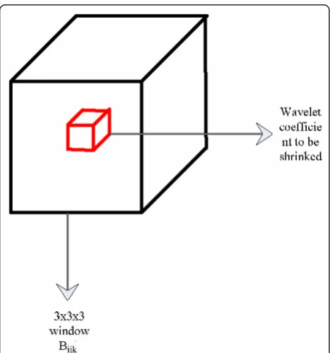
For the 3D wavelet wijkcoefficient to be shrunk,

con-sider a cubic neighborhood Bijk centered at wijk, as

shown in Figure 3. The size of neighborhood is

repre-sented as 3 × 3 × 3. For S2ijk =

(p,q,m)∈Bijk

w2_pqm_{, the}

NeighShrink shrinkage formula is given by [29]

θijk=wijkmax

1− λ

2

S2_ijk, 0

(12)

where θijk is the estimator of the unknown noiseless

coefficient and l is the threshold. The optimall for each of the high-frequency subbands is estimated using SURE.

In the Neighshrink method, all the wavelet coefficients are shrunk to achieve the purpose of denoising. The

Figure 2Modified neighborhood in 3D wavelet domain.

(5)

result of this may be the noise is reduced while the structural details important in medical image are blurred. As shown in a previous study [29], the over-smoothing could be compensated by exploiting the neighborhood statistics over a pixel to be denoised. By taking advantage of the essential feature of wavelet coef-ficients known as energy clustering within each subband, a 3D WNS method was proposed to preserve the struc-tural information in MRI.

Let WDi

pqm denotes the wavelet coefficient at location

(p,q,m) in subband Di which belongs to {LxHyHz, HxLyHz,HxHyLz,HxHyHz}, andKLHH, KHLH, KHHL, KHHH represent different weights of different wavelet sub-bands, respectively, as shown in Figure 4. Weighting fac-tors were determined according to the 3D Directional Filter Banks (3D DFB) developed by Lu and Do [30]. Then, SDi

ijk will be calculated as follows:

SDi

ijk= ⎧ ⎪ ⎪ ⎪ ⎪ ⎪ ⎪ ⎪ ⎪ ⎪ ⎪ ⎨ ⎪ ⎪ ⎪ ⎪ ⎪ ⎪ ⎪ ⎪ ⎪ ⎪ ⎩

(p,q,m)∈Bijk

KLHH(WDi

pqm)

2

Di∈LxHyHz

(p,q,m)∈Bijk

KHLH_(WDi

pqm)

2

Di∈HxLyHz

(p,q,m)∈Bijk

KHHL_(WDi

pqm)

2

Di∈HxHyLz

(p,q,m)∈Bijk

KHHH_(WDi

pqm)

2

Di∈HxHyHz

(13)

The estimator of the unknown noiseless coefficient

θijk is determined according to Equation (12).

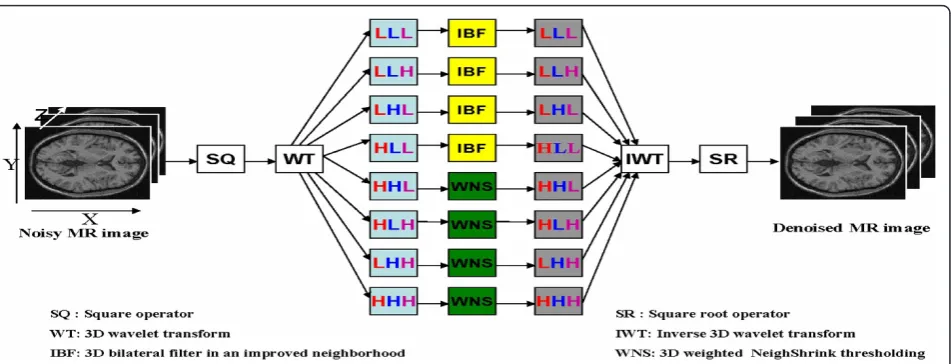
2.5. Algorithm summary

The proposed 3D wavelet domain improved bilateral fil-ter with the WNS thresholding (3DW-IBF) was sum-marized as follows (see Figure 5):

(1) Compute the square of noisy MR imageIto obtain its square magnitudeIsq.

(2) Use 3D WT to get the approximation coefficients (LxLyLz, LxLyHz, LxHyLz, LxLyHz) and the detail coeffi-cients (LxHyHz, HxLyHz, HxHyLz, HxHyHz) ofIsq(see

Sec-tion 2.2).

(3) The bias in approximation coefficients is removed by subtracting 4σ_n2[15] (see Section 2.1).

(4) These unbiased approximation coefficients are passed through the 3D improved bilateral filter (see Sec-tion 2.3).

(5) Denoise the detail coefficients using 3D WNS thresholding technique (see Section 2.4).

(6) Compute inverse 3D WT of the filtered approxi-mation and the denoised detail coefficients to obtain the estimate ofIsq(see Section 2.2).

(7) The square root of the resultant gives the denoised magnitude MR image.

3. Experiments and results

3.1. Experimental data description

We have carried out experiments with both simulated and real data. To conduct the experiments over syn-thetic data, three simulated MR images (T1, T2 and PD) with 1 mm3 voxel resolution (8-bit quantization) from the Brainweb phantom [31] were used. Each image con-tained 181 × 217 × 181 voxels. To simulate Rician noise, we added zero mean Gaussian noise to the real and imaginary parts of the simulated MR data and after-wards the magnitude image was computed.

To evaluate the proposed approach on real clinical data, three datasets were used. Informed consent was obtained from all volunteers in accordance with our institution’s policies regarding human subjects. The first dataset consisted of an MP-RAGE T1w volumetric sequence (256 × 240 × 176 voxels with a voxels resolu-tion of 1 mm3) acquired on a Siemens 1.5T Vision scan-ner. The acquisition parameters were TR = 9 ms, TE = 4 ms, flip angle = 10°, TI = 2 ms, TD = 200 ms.

The second dataset was obtained with a TSE-FLAIR volumetric sequence (256 × 256 × 160 voxels with a vox-els resolution of 0.94 × 0.94 × 1 mm3) acquired on a Phi-lips Gyroscan 3 Tesla scanner (Best, Netherlands) using a sensitivity encoding (SENSE) acceleration factor of 2, TR = 14 ms, and TE = 140 ms. Although parallel acquisition techniques such as SENSE or generalized autocalibrating partially parallel acquisitions introduce a spatially varying noise variance across the image, we used this dataset here to show the capability of the proposed approach on MR images with spatially varying noise.

Finally, we have obtained an image with a particularly large amount of noise by courtesy of Huiping Shi (Qiqi-haer Medical College, Qiqi(Qiqi-haer, China), as to assess the performance of the methods under extreme conditions. It was obtained on a 0.5 Tesla Neusoft-Philips, with para-meters TR = 20 ms, TE = 5 ms, flip angle = 90°, field of view = 26 cm, matrix = 256 × 160, slice thickness = 2 mm. The resulting 3D image has size 512 × 512 × 40 voxels. Its original values are in the range [0, 255].

3.2. Quantitative and qualitative metrics

The efficiency of the denoising methods was compared quantitatively and qualitatively. For quantitative assess-ment, the mean squared error (MSE) and the Structural Similarity index (SSIM) [32] were evaluated. These mea-sures were computed with the noise-free MR images as the ground truth. MSE is an objective measure that quan-tifies the deviation of estimated values from the true value

MSE = 1

M

i=1

(6)

whereI(i) and I0(i) are the pixel (voxel) values at

posi-tion i of the original image and the denoised image, respectively. M denotes the number of the pixels in each image. MSE yields the same relative ordering among methods as the power signal-to-noise ratio (PSNR) and the root mean squared error (RMSE):

PSNR = 10log₁₀255

2

MSE (15)

RMSE =√MSE (16)

(7)

with the visual perception. As mentioned in previous section, MRI consists of delicate structural details, for which MSE is not sufficient to quantify the restored information. Therefore, SSIM is also used to study the structural and perceptual closeness between the denoised and the original images. The SSIM index is estimated locally over a 11 × 11 window, which moves pixel-by-pixel over the entire image. The final value of SSIM is the mean of SSIM index calculated over theN local regions. The SSIM between the image X andYis calculated from

SSIM(x,y)N=

(2μxμy+c1)(2δxy+c2)

(μ2

x+μ2y +c1)(δ2x+δ2y +c2) (17)

whereμ is the mean intensity,δdenotes the standard deviation, and the constantsc1 = 0.01, c2 = 0.03 were

chosen as recommended in Wang et al. [32].

SSIM(X,Y) = 1 N

N

R=1

SSIM(x,y)R (18)

The value of SSIM lies between [-1, 1]. Alternatively, the SSIM can also be given in percentage (%). Larger value of SSIM means high similarity between the com-pared images.

Visual assessment of the residual image was employed for qualitative evaluation. The residual image was obtained by subtracting the denoised image from the noisy image [12]. The residual image was required to verify the traces of anatomical information in clinical image removed during denoising. So, this could reveal the excessive smoothing and blurring of small structural details contained in the image.

3.3. Validation on simulated dataset

We have compared, qualitative and quantitatively the performance of our proposed algorithm with optimal estimated parameters (Rneighbor = 7,δd = 5,δr= 1.5sn)

with other three state-of-the-art filtering algorithms: the unbiased nonlocal means filter (UNLM) [12], the adap-tive blockwise non-local means filter (ABONLM) [9], and the 2D wavelet domain bilateral filter (2DW-BF) [19].

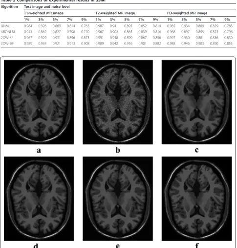
Our algorithm was quantitatively compared, using the synthetic data referred in Section 3.1. The values of MSE and SSIM obtained for the synthetic data using the aforementioned denoising techniques were tabulated in Tables 1 and 2, respectively. The performance of 3DW-IBF with weighted Neighshrink is better than UNLM, ABONLM, and 2DW-BF with respect to the quantitative metrics. Lower value of MSE and higher value of SSIM showed that our method significantly outperforms others.

The results on T1-weighted images were shown in Figure 6. The original MR image (Figure 6a) and the noisy image with 5% Rician noise added (Figure 6b) were presented. Some structural details were smoothed in the results obtained by the UNLM filter (Figure 6c). While the UNLM filter could preserve the distinct edge features, it failed to preserve small structural details. The results obtained by the ABONLM filter (Figure 6d) were better than those by the UNLM filter. However, some regions were blurred and some useful information was lost. We found that the 2D-WBF filter has the coarse edge effect (Figure 6e) compared to our proposed filter (Figure 6f).

(8)

Table 1 Comparisons of experimental results in MSE

Algorithm Test image and noise level

T1-weighted MR image T2-weighted MR image PD-weighted MR image

1% 3% 5% 7% 9% 1% 3% 5% 7% 9% 1% 3% 5% 7% 9% UNML 2.50 11.42 24.71 43.69 68.12 3.31 18.62 38.68 64.97 97.78 2.68 13.85 29.52 48.78 71.20 ABONLM 3.28 19.78 51.07 97.98 161.39 6.55 24.76 56.19 101.03 159.83 4.01 18.82 46.08 87.25 141.02 2DW-BF 3.08 11.56 26.06 51.56 62.26 7.23 20.33 57.30 68.27 90.03 3.65 15.19 30.63 43.67 62.77 3DW-IBF 2.07 8.20 15.11 22.31 29.58 4.62 15.54 29.21 50.10 67.38 3.52 11.18 20.65 26.12 41.58

Table 2 Comparisons of experimental results in SSIM

Algorithm Test image and noise level

T1-weighted MR image T2-weighted MR image PD-weighted MR image

1% 3% 5% 7% 9% 1% 3% 5% 7% 9% 1% 3% 5% 7% 9% UNML 0.984 0.926 0.869 0.814 0.763 0.987 0.941 0.895 0.852 0.814 0.985 0.934 0.880 0.829 0.783 ABONLM 0.943 0.862 0.827 0.798 0.770 0.967 0.902 0.865 0.839 0.816 0.968 0.897 0.855 0.823 0.796 2DW-BF 0.967 0.929 0.931 0.896 0.873 0.991 0.948 0.899 0.867 0.856 0.997 0.930 0.881 0.836 0.830 3DW-IBF 0.989 0.934 0.921 0.913 0.908 0.989 0.942 0.916 0.901 0.882 0.988 0.946 0.903 0.890 0.855

(9)

obtained by the 2DW-BF filter (Figure 7e) reserved more information than the result obtained by the UNLM filter (Figure 7c) and that obtained by the ABONLM filter (Figure 7d). However, the 2DW-BF fil-ter smoothed the homogeneous regions. We observed that the result obtained by our proposed filter (Figure 7f) could recover as much information as that by the 2DW-BF filter.

The results on PD-weighted image were shown in Fig-ure 8. The noisy image with 9% Rician noise added was presented (Figure 8b). We found that the interface between gray and white matter in the result by the UNLM filter (Figure 8c) was away from that of the ori-ginal image (Figure 8a), and the result by the ABONLM filter (Figure 8d) was oversmoothed. There was still some obvious noise in the result by the 2DW-BF filter (Figure 8e). Both the small structures and the

boundaries were preserved well by the 3DW-IBF filter (Figure 8f).

3.5. Validation on clinical dataset

Since the original images already have noise, neither ideal residual image nor quantitative results can be obtained. The denoising results obtained for the T1-weighted brain image were shown in Figure 9. The resi-dual images of the UNLM filter (Figure 9c), the ABONLM filter (Figure 9e), and the 3DW-IBF method (Figure 9i) did not reveal significant anatomical informa-tion. The residual image of the 2DW-BF filter showed the extent of smoothing along the edges of the image (Figure 9g). While the 2DW-BF filter could preserve the distinct edge features, it blurs the heterogeneous regions and hence, reduces the contrast between the gray and the white matter regions. The results of filtering SENSE

(10)

images reconstructed from patient brain data were shown in Figure 10. The ULM filter and the 2DW-BF method left unfiltered noise in the image (Figure 10b, f). With the ABONLM method, the edges were blurred, reducing the image sharpness (Figure 10d). Alterna-tively, with the 3DW-IBF method, the edges were pre-served well and the contrast between the gray and the white tissues were also preserved well (Figure 10h). The results obtained for the T1-weighted brain image with heavy noise were shown in Figure 11. With the 2DW-BF method, the sharpness along the edges was smoothed (Figure 11f). Comparing the results of the ULM filter (Figure 11b) and the ABONLM method (Fig-ure 11d), it was evident that the 3DW-IBF method pre-serves well the details (Figure 11h).

4. Discussion and conclusion

(11)

the MR measurement due to thermal noise. But we expected to estimate the variance component due to physiological noise such as flow, MR spin history effect. To this end, it requires many repeated acquisitions. It would also be difficult to isolate the variance due to patient motion in such repeated measurements (which is something the registration step is actually trying to diminish). Therefore, we did not estimate the noise introduced by physiological effects.

(12)

Consider a slender fiber tract. If the imaging plane is orthogonal to the fiber axis, it would be much more dif-ficult to distinguish the “structure” from spurious, bright, noise pixel. 3D denoising uses structural correla-tions from all three principle planes, and is robust to fiber axis orientation.

Considering the similarities in the wavelet domain where the data and noise can be efficiently discrimi-nated, 3D bilateral filtering of the approximation coeffi-cients in a modified neighborhood eliminates the higher magnitude noise components carried into the approxi-mation subbands. Utilizing a group of a square and a line as neighbor to replace the original cubic neighbor for weight estimation improves the computation accu-racy. Noticing the fact that the wavelet subband coeffi-cients of different orientations have different properties

of energy clustering, a WNS thresholding has been pro-posed to threshold the noisy coefficients in the detailed subbands. Exploiting the interscale dependencies among the detailed coefficients tends to improve the perfor-mance of wavelet thresholding, and thus, it also enhances the denoising efficiency for MR images with spatially varying noise. In summary, the utilization of neighborhood similarities using wavelet domain bilateral filter and Neighshrink improves the noise cancellation efficiency and preserves the structural information effectively.

Experiments were carried out on both simulated and real datasets. Quantitative results using two different quality measures show a better behavior of the proposed scheme when compared to other state-of-the-art filters for different noise levels.

(13)

An ideal filter for MR images with spatially varying noise levels must be able to improve the image PSNR while preserving image important structures and avoid-ing the generation of artifacts. The results indicated that parametersnchosen as a constant in all image areas may

lead to the enhancement of noise-generated gradients in high-noise areas that could be incorrectly identified as anatomical structures of different tissue type characteris-tics for the imaging modality such as vessels. Therefore, it is necessary to derive a strategy that optimizes the choice ofsnwith respect to the local characteristics of

the considered neighborhoods. Hence, this study can be extended to make the choice ofsnlocally adaptive,

opti-mizing the denoising procedure for all the noise levels.

Acknowledgements

We would like to thank McConnell Brain Imaging Center (BIC) of the Montreal Neurological Institute, McGill University, for providing access to the MR data in the BrainWeb Database (http://www.bic.mni.mcgill.ca/brainweb). We would also like to thank VisAGeS of the IRISA Institute, University of Rennes I, for providing online applications (http://www.irisa.fr/visages/ benchmarks/).

Author details

1

Department of Computational Mathematics, Jilin University, Chang chun, China2_{Department of Clinical Medicine, Qiqihaer Medical College, Qiqihaer,}

China

Competing interests

The authors declare that they have no competing interests.

Received: 20 July 2011 Accepted: 21 February 2012 Published: 21 February 2012

(14)

References

1. G McGibney, MR Smith, An unbiased signal-to-noise ratio measure for magnetic resonance images. Med Phys.20(4), 1077–1078 (1993). doi:10.1118/1.597004

2. J Sijbers, AJ Dekker, Maximum likelihood estimation of signal amplitude and noise variance from MR data. Magn Reson Med.51(3), 586_–594 (2004). doi:10.1002/mrm.10728

3. P Perona, J Malik, Scale-space and edge detection using anisotropic diffusion. IEEE Trans Pattern Anal Mach Intell.12(7), 629–639 (1990). doi:10.1109/34.56205

4. G Gerig, O Kubler, R Kikinis, FA Jolesz, Nonlinear anisotropic filtering of MRI data. IEEE Trans Med Imag.11(2), 221–232 (1992). doi:10.1109/42.141646 5. AA Samsonov, CR Johnson, Noise-adaptive nonlinear diffusion filtering of

MR images with spatially varying noise levels. Magn Reson Med.52(4), 798_–806 (2004). doi:10.1002/mrm.20207

6. K Krissianand, S Aja-Fernández, Noise-driven anisotropic diffusion of noisy MRI data. IEEE Trans Image Process.18(10), 2265_–2274 (2009)

7. M Martin-Fernandez, C Alberola-Lopez, J Ruiz-Alzola, CF Westin, Sequential anisotropic Wiener filtering applied to 3D MRI data. Magn Reson Imag. 25(2), 278–292 (2007). doi:10.1016/j.mri.2006.05.001

8. P Coupé, P Yger, S Prima, P Hellier, C Kervrann, C Barillot, An optimized blockwise non local means denoising filter for 3D magnetic resonance images. IEEE Trans Med Imag.27(4), 425–441 (2008)

9. JV Manjón, P Coupé, L Martí-Bonmatí, DL Collins, M Robles, Adaptive non-local means denoising of MR images with spatially varying noise levels. J Magn Reson Imag.31(1), 192_–203 (2010). doi:10.1002/jmri.22003 10. A Buades, B Coll, J-M Morel, A non-local algorithm for image denoising, in

CVPR 2005, San Diego, USA, 60_–65 (June 2005)

11. N Wiest-Daesslé, S Prima, P Coupé, SP Morrissey, C Barillot, Rician noise removal by non-local means filtering for low signal-to-noise ratio MRI: applications to DT-MRI, inMICCAI 2008, New York, USA, 104–117 (September 2008)

12. JV Manjón, J Carbonell-Caballero, JJ Lull, G García-Martí, L Martí-Bonmatí, M Robles, MRI denoising using non-local means. Med Image Anal.12(4), 514_–523 (2008). doi:10.1016/j.media.2008.02.004

13. AM Wink, JBTM Roerdink, Denoising functional MR images: a comparison of wavelet denoising and Gaussian smoothing. IEEE Trans Med Imag.23, 374–387 (2004). doi:10.1109/TMI.2004.824234

14. A Pizurica, AM Wink, E Vansteenkiste, W Philips, J Roerdink, A review of wavelet denoising in MRI and ultrasound brain imaging. Curr Med Imag Rev.2(2), 247–260 (2006). doi:10.2174/157340506776930665

15. RD Nowak, Wavelet-based Rician noise removal for magnetic. IEEE Trans Image Process.8(10), 1408–1419 (1999). doi:10.1109/83.791966 16. P Bao, L Zhang, Noise reduction for magnetic resonance images via

adaptive multiscale products thresholding. IEEE Trans Med Imag.22(9), 1089_–1099 (2003). doi:10.1109/TMI.2003.816958

17. S Zaroubi, G Goelman, Complex denoising of MR data via wavelet analysis: application for functional MRI. Magn Reson Imag.18(1), 59_–68 (2000). doi:10.1016/S0730-725X(99)00100-9

18. ZQ Wu, JA Ware, J Jiang, Wavelet-based Rayleigh background removal in MRI. Electron Lett.39(7), 603–605 (2003). doi:10.1049/el:20030396 19. CS Anand, JS Sahambi, Wavelet domain non-linear filtering for MRI

denoising. Magn Reson Med.28(6), 842_–861 (2010)

20. X Yang, B Fei, A wavelet multiscale denoising algorithm for magnetic resonance (MR) images. Meas Sci Technol.22, 025803 (2011). doi:10.1088/ 0957-0233/22/2/025803

21. H Gudbjartsson, S Patz, The Rician distribution of noisy MRI data. Magn Reson Med.34, 910–914 (1995). doi:10.1002/mrm.1910340618

22. S Aja-Fernández, C Alberola-López, CF Westin, Noise and signal estimation in magnitude MRI and Rician distributed images: a LMMSE approach. IEEE Trans Image Process.17(8), 383–398 (2008)

23. M Brummer, R Mersereau, R Eisner, R Lewine, Automatic detection of brain contours in MRI data sets. IEEE Trans Med Imag.2(29), 153–166 (1993) 24. J Sijbers, D Poot, AJ den Dekker, W Pintjens, Automatic estimation of the

noise variance from the histogram of a magnetic resonance image. Phys Med Biol.52, 1335_–1348 (2007). doi:10.1088/0031-9155/52/5/009 25. J Sijbers, AJ den Dekker, J Van Audekerke, M Verhoye, D Van Dyck,

Estimation of the noise in magnitude MR images. Magn Reson Imag.1(16), 87–90 (1998)

26. Z Chen, R Ning, Breast volume denoising and noise characterization by 3D wavelet transform. Comput Med Imag Graph.28, 235–246 (2004). doi:10.1016/j.compmedimag.2004.04.004

27. C Tomasi, R Manduchi, Bilateral filtering for gray and color images, inICCV 1998, Bombay, India, 839–846 (January 1998)

28. GY Chen, TD Bui, A Krzyzak, Image denoising with neighbour dependency and customized wavelet and threshold. Pattern Recogn.38, 115–124 (2005). doi:10.1016/j.patcog.2004.05.009

29. D Zhou, W Cheng, Image denoising with an optimal threshold and neighbouring window. Pattern Recogn Lett.29(11), 1694–1697 (2008). doi:10.1016/j.patrec.2008.04.014

30. Y Lu, MN Do, Multidimensional directional filter banks and surfacelets. IEEE Trans Image Process.16(4), 918–931 (2007)

31. DL Collins, AP Zijdenbos, V Kollokian, JG Sled, NJ Kabani, CJ Holmes, AC Evans, Design and construction of a realistic digital brain phantom. IEEE Trans Med Imag.17(3), 463–468 (1998). doi:10.1109/42.712135

32. Z Wang, AC Bovik, HR Sheikh, EP Simoncelli, Image quality assessment: from error visibility to structural similarity. IEEE Trans Image Process.13(4), 600_–612 (2004). doi:10.1109/TIP.2003.819861

doi:10.1186/1687-6180-2012-40

Cite this article as:Wanget al.:Nonlinear filtering based on 3D wavelet

transform for MRI denoising.EURASIP Journal on Advances in Signal

Processing20122012:40.