Volume 2009, Article ID 261542,17pages doi:10.1155/2009/261542
Research Article
Facial Expression Biometrics Using Statistical Shape Models
Wei Quan, Bogdan J. Matuszewski (EURASIP Member), Lik-Kwan Shark,
and Djamel Ait-Boudaoud
Applied Digital Signal and Image Processing Research Centre, University of Central Lancashire, Preston PR1 2HE, UK
Correspondence should be addressed to Bogdan J. Matuszewski,[email protected]
Received 30 September 2008; Revised 2 April 2009; Accepted 18 August 2009
Recommended by Jonathon Phillips
This paper describes a novel method for representing different facial expressions based on the shape space vector (SSV) of the statistical shape model (SSM) built from 3D facial data. The method relies only on the 3D shape, with texture information not being used in any part of the algorithm, that makes it inherently invariant to changes in the background, illumination, and to some extent viewing angle variations. To evaluate the proposed method, two comprehensive 3D facial data sets have been used for the testing. The experimental results show that the SSV not only controls the shape variations but also captures the expressive characteristic of the faces and can be used as a significant feature for facial expression recognition. Finally the paper suggests improvements of the SSV discriminatory characteristics by using 3D facial sequences rather than 3D stills.
Copyright © 2009 Wei Quan et al. This is an open access article distributed under the Creative Commons Attribution License, which permits unrestricted use, distribution, and reproduction in any medium, provided the original work is properly cited.
1. Introduction
Facial expressions provide important information in com-munication between people and can be used to enable communication with computers in a more natural way. Recent advances in imaging technology and ever increasing computing power have opened up a possibility of automatic facial expression recognition. Up till now some research efforts have been exploited in applications such as human-computer interaction (HCI) systems [1], video conferenc-ing [2], and augmented reality [3]. From the biometric perspective, the automatic expression recognition has been investigated in the context of patients’ monitoring in the intensive care and neonatal units [4] for signs of pain and anxiety, behavioural research on children’s ability to learn emotions by interacting with adults in different social contexts [5], identifying level of concentration [6], that is, for detecting drivers’ tiredness, and finally in aiding face recognition. Facial expression representation, which forms one of the most important elements in the facial expression recognition system, is concerned with extraction of facial features for representing variations of expressions. Good features for representing the facial expressions should enable interpretation of various face articulations without any limitation of race, gender, and age. Furthermore, it
should also have the capability of reducing the complexity of classification algorithms.
of landmarks localised around the facial features such as eyebrows, eyes, mouth, and nose [11]. As an extension of the AAM, the 3D morphable model was developed by Blanz and Vetter [12]. Instead of using manually selected sparse facial landmarks, the 3D morphable model uses all the data points of 3D facial scans to represent the geometrical information. This model has been used to control 3D facial surfaces from a 2D image, across variations in pose, ranging from frontal to profile view, and a wide range of illuminations. B-spline is a parametric model which is often used to describe surfaces. When used with 3D facial data, a large number of data points can be efficiently modelled by a small number of B-spline’s control points [13]. When combined with the facial action coding system (FACS) [14], the control points are placed in areas that correspond to action units, and the expression of a face can be generated automatically by adjusting the B-spline’s control points.
In contrast to the holistic approaches, the local repre-sentation methods focus on the local features or areas that are prone to change with facial expressions. Saxena et al. [15] introduced the localised geometric model to locally represent facial expressions. Their method uses the classical edge detectors with colour analysis for extracting the local appearances of a face such as eyebrows, lips, and nose. Subsequently a feature vector containing measurements of the facial appearances, such as the height of eyebrows, brow distance, mouth height, mouth width, and lip curvature, is created for the facial expression classification. A local parameterised model proposed by Black and Yacoob [16] is developed based on image motion which is calculated using the optical flow of facial image sequences. The image motion not only accurately models a nonrigid facial motion but also provides a concise description that is related to the motion of local facial features to recognise facial expressions. Kobayashi et al. [17] used a point-based geometric model for the facial expression representation. The model contains 30 facial characteristic points in the frontal-view of the face. These facial characteristic points are around the areas that are the most affected by change of facial expressions, such as eyes, nose, brows, and mouth.
In this paper, a novel method for representing facial expressions is proposed based on the authors’ previous work [18–20], which postulates that the shape space vectors constitute a significant feature space for the recognition of facial expressions. The proposed method uses only 3D shape information, with the texture not being used at all. The method is therefore inherently invariant to variations in scene illumination conditions, background clutter, and to some extent angle of view. This is in a striking contrast to the methods based on texture where these factors severely limit their practical applicability. Additionally as the texture is not being used, it does not have to be captured; hence fast full frame 3D acquisition techniques based on the time-of-fly principle [21] can be used (3D scanners capturing in excess of 40 frames/sec are commercially available) instead of more computationally intensive, and therefore slower, stereovision scanning systems. The shape space vector (SSV) is the key element in the statistical shape model (SSM), which models the high-dimensional shape variations
observed in the training data set using projections on a low-dimensional shape space. In order to obtain the SSV two consecutive stages are necessary, namely, (i) model building stage and (ii) model fitting stage. In the model building stage, the correspondences of points between all faces present in the training data set are established first so that the training data set can be aligned into a common reference face. Subsequently the principal component analysis (PCA) technique is applied to the aligned training data set to obtain the SSM of the shape variations. In the model fitting stage, an iterative algorithm based on a modified iterative closest point (ICP) method is used to gradually adjust the pose parameters and optimise the shape parameters in order to match the model to the newly observed facial data. The pose parameters consist of a translation vector, a rotation matrix, and a scaling factor, whereas the shape parameters are embedded in the SSV. In order to validate the discriminatory ability of the SSV, 3D synthetic faces generated from the FaceGen Modeller [22] and real 3D facial scans from the BU-3DFE database [23] are used for the separability analysis in the SSV domain. The experiments on recognition of facial expressions using a selection of standard classification tools are also presented.
The remainder of this paper is organised as follows. Section 2 introduces the details of construction of the SSM.Section 3describes the procedure used for fitting the model to the facial data that has not been included in the training data set.Section 4provides results of qualitative and quantitative separability analysis. Results of facial expression recognition using some popular classification algorithms operating on the SSV feature space are presented inSection 5. Finally, concluding remarks are given in Section 6, and a potential improvement of the expression representation using the SSV constructed for dynamic 3D data is briefly discussed inSection 7.
2. Statistical Shape Model
The statistical shape model (SSM) is developed based on the point distribution model (PDM) which was proposed by Cootes et al. [24], and it is one of the most widely used techniques for the model-based data representation and registration. The model describes shape variations based on the statistic calculated from the position of the corresponding points in the training data set. In order to build an SSM, the correspondence of points between different 3D faces in the training data set must be estab-lished first. Subsequently the principal component analysis (PCA) is applied to the mutually aligned training data set.
Reference face
Training faces TPS warping
TPS warping
TPS
warping Closestpoint matching
Closest point matching
Closest point matching
Corresponded training faces
Figure1: Example of point correspondence estimation in the training data set, with example images from the BU-3DFE.
is explicitly provided by the software, whereas the dense correspondence of points for the faces in the BU-3DFE database is estimated based on a set of facial landmarks included in the database.
In this work, the estimation of the correspondence is achieved in three steps: (i) facial landmark determination, (ii) thin-plate spline (TPS) warping, and (iii) closest point matching. The first step is to identify the corresponding facial landmarks on the reference and training faces. The second step is to warp the reference face to different training face using TPS transformation that is calculated based on the selected facial landmarks as control points [25]. The last step is to estimate the point correspondence between the warped reference face and different training faces based on the closest distance metric. Figure 1 shows the framework of computing the dense point correspondence of different training faces from the BU-3DFE database. The reference face is usually selected as a face containing neutral expression with the mouth closed. Such selection of the reference face helps to avoid wrong correspondences in the case of matching between closed-mouth and open-mouth shapes. If the reference face were selected with the mouth open, after dense correspondence estimation, each point in the open-mouth area of the reference face will find an incorrect corresponding point in the training face within the closed-mouth region even though those corresponding points of the open-mouth area do not exist in the training faces with mouth closed.
2.1.1. Thin-Plate-Spline Warping. The TPS warping tech-nique is a point-based registration method which was first
proposed by Bookstein [26]. The TPS warping can be used for interpolation as well as approximation. For the TPS interpolation, the positions of corresponding landmarks are assumed to be known exactly and the corresponding landmarks are forced to match exactly each other after warping [25,27]. For the TPS approximation, the landmark position errors are taken into account, implying that the corresponding landmarks are not forced to match exactly after warping is applied. It can be shown that the solution of the approximation problem is equivalent to inclusion of a regularisation term in the cost function along with a fidelity term which is exactly the same as used in the definition of the interpolation problem [28]. In this work, the corresponding facial landmarks are manually labeled on the 3D face scans, and their positions are always prone to some errors. Therefore, the TPS approximation model is more suitable for our application.
Given sparse corresponding facial landmarks in the reference face and one of the training faces, repre-sented, respectively, by P = (p1,p2,. . .,pL)T and Q =
(q1,q2, . . .,qL)T, where pk = (xpk,ypk,zpk)T and qk =
(xqk,yqk,zqk)Tdenotex,y, andzcoordinates of thekth
cor-responding pair andLis the total number of corresponding facial landmarks, the objective is to find the TPS warping function that warps the reference face to the training face. The interpolating warping function, F, has to fulfill the following constraint for all the landmarks inPandQ:
Fpi
where the deformation model is defined in terms of warping functionF(pj) with
Fpj
= ⎡ ⎢ ⎢ ⎢ ⎢ ⎣ fx pj fy pj fz pj ⎤ ⎥ ⎥ ⎥ ⎥
⎦, (2)
wherepj=(xp j,yp j,zp j)Tis a point on the reference face and
the warping functions forx,y, andzcoordinates are defined as follows
fx
pj
=a+axxp j+ayyp j+azzp j
+
L
i=1
wxiUpi−pj
, (3) fy pj
=b+bxxp j+byyp j+bzzp j
+
L
i=1
wyiUpi−pj
, (4) fz pj
=c+cxxp j+cyyp j+czzp j
+
L
i=1
wziUpi−pj
.
(5)
FunctionUis a radial basis function of the form
U(r)=r2logr2, (6)
where r is a distance between two points. According to Bookstein [26], the coefficients of the TPS interpolation model can be calculated from
KcWc+PcAc=Q, (7)
and
PT
cWc=0, (8)
whereQis aL×3 matrix which contains facial landmarks on the target face and written as
Q= ⎡ ⎢ ⎢ ⎢ ⎢ ⎢ ⎢ ⎣
xq1 yq1 zq1
xq2 yq2 zq2
· · · ·
xqL yqL zqL
⎤ ⎥ ⎥ ⎥ ⎥ ⎥ ⎥ ⎦ . (9)
WcandAcare the matrices containing coefficients of the TPS
interpolation and defined as
Wc=
⎡ ⎢ ⎢ ⎢ ⎢ ⎢ ⎢ ⎣
wx1 wy1 wz1
wx2 wy2 wz2
· · · · wxL wyL wzL
⎤ ⎥ ⎥ ⎥ ⎥ ⎥ ⎥ ⎦
, Ac=
⎡ ⎢ ⎢ ⎢ ⎢ ⎢ ⎢ ⎣
a b c
ax bx cx
ay by cy
az bz cz
⎤ ⎥ ⎥ ⎥ ⎥ ⎥ ⎥ ⎦ , (10)
whereas matrixKcthat contains the radial basis functions is
defined as
Kc=
⎡ ⎢ ⎢ ⎢ ⎢ ⎢ ⎢ ⎣
U(r11) U(r12) · · · U(r1L)
U(r21) U(r22) · · · U(r2L)
· · · · · · · · · · · · U(rL1) U(rL2) · · · U(rLL)
⎤ ⎥ ⎥ ⎥ ⎥ ⎥ ⎥ ⎦ , (11)
and the radial basis functionU(ri j) is
Uri j
=pi−qj
2
logpi−qj
2
. (12)
Pcis the matrix including all corresponding landmarks of the
reference face and defined as
Pc=
1P, (13)
and matrixPis defined as
P= ⎡ ⎢ ⎢ ⎢ ⎢ ⎢ ⎢ ⎣
xp1 yp1 zp1
xp2 yp2 zp2
· · · ·
xpL ypL zpL
⎤ ⎥ ⎥ ⎥ ⎥ ⎥ ⎥ ⎦ . (14)
In the TPS approximation model, the interpolation condition has to be weakened since the landmark localisation errors have to be taken into account. The regularisation term needs to be added into the TPS interpolation model in order to control smoothness of the transformation. The coefficients of the TPS approximation model can be calculated as
(Kc+λcI)Wc+PcAc=Q, (15)
where λc > 0 is a relative weighting factor between the
interpolating behavior and the smoothness of the transfor-mation. For small λc, the TPS warping maintains a good
approximation of the landmarks. For large λc, the TPS
warping function becomes very smooth and adopts very little to the local structures present in the data.
2.1.2. Closest Point Matching. After the TPS approximation, the shape of the reference face is warped to match the training face. Since the shape of the reference face is close to the shape of the training face, the dense point correspondence of the reference face for the training face can be computed using the closest distance metric. With the Euclidean distanced(p,q) between two points p = (xp,yp,zp)T andq =(xq,yq,zq)T
are defined as
dp,q=xp−xq
2
+yp−yq
2
+zp−zq
2
. (16)
Denoting a set of points of the training face by {qi,i ∈
[1,N]}, the closest distance between a pointp=(xp,yp,zp)T
of the reference face and the training face is defined as
dp,qi,i∈[1,N]
=arg min
i
dp,qi
Using the TPS approximation and closest point match-ing, the dense point correspondence between the reference face and a training face can be established. This process is applied to all the training faces such that all of them are in correspondence. The training faces from the BU-3DFE database contain between 13 000 and 20 000 mesh polygons with 8711 to 9325 vertices. The reference face used in this paper has 15 687 mesh polygons and 8925 vertices. After performing the TPS approximation and closest point matching, it is likely that there will be multi-to-one correspondences between a training face and the reference face. It is impossible to avoid this completely due to the nature of the closest point matching technique. In order to reduce the number of such correspondences, a subdivision surface method has been used to increase the number of vertices in the training faces [29].
2.2. Principal Component Analysis. Using the standard prin-cipal component analysis (PCA), each 3D face in the training data set can be approximately represented in a low-dimensional shape vector space [30] instead of the original high-dimensional data vector space. Given a training data set of M faces, Qi(i = 1, 2,. . .,M), each containing N
corresponding data pointsQi ∈R3N, whereQicontains all
the data points of theith face encoded as a 3N-dimensional vector. The first step of the PCA is to calculate the mean vectorQ(representing the mean 3D face):
Q= 1 M
M
i=1
Qi. (18)
LetCbe defined as the covariance matrix calculated from the training data set:
C= 1
M
M
i=1
Qi−Q
Qi−Q
T
. (19)
By building a matrixXof “centered” data vectors withQi−Q
as theith column of matrixX, covariance matrixCcan be calculated as
C=XXT, (20)
where matrix C has 3N rows and columns. Since the number of faces, M, in the training data set is smaller than the number of data points, the eigen decomposition of matrix C = XTX is performed first [31]. The first M
largest eigenvaluesλi(i =1,. . .,M) and eigenvectorsui(i =
1,. . .,M) of the original covariance matrix, C, are then determined, respectively, from
λi=λi, (21)
ui= Xu
i
Xu
i
, (22)
whereλi andui are eigenvalues and eigenvectors of matrix
C, respectively. By using these eigenvalues and eigenvectors, the data points on any 3D face in the training data set can be approximately represented using a linear model of the form
Q=Wb+Q, (23)
where W = [u1,. . .,ui,. . .,uK] is a 3N × K so-called
“Shape Matrix” ofK eigenvectors, or “modes of variation”, which correspond to the K largest eigenvalues, and b =
[b1,. . .,bi,. . .,bK] is the shape space vector (SSV), which
controls contribution of each eigenvector,ui, in the
approx-imated surface Q [12]. The shape matrix W is database-dependent. In a case when new faces are added to the existing database, this shape matrix needs to be recalculated. Most of the surface variations can usually be modelled by a small number of modesK. Equation (23) can be used to generate new examples of faces by changing the SSV,b, with suitable limits [24]. According to the work proposed by Edwards et al. [11], the suitable limits of the SSM are typically defined as
−3
λi≤bi≤3
λi. (24)
Figure 2 shows the effect of varying the first three largest principal components of the two models. These models were built using 450 training faces from the FaceGen and BU-3DFE database, respectively.
3. Model Fitting
Provided that the faces in the database are representative of the faces in the population, a new face from the same population, which has not been included in the training data, can be represented using the derived SSM. In the proposed method, the model fitting is treated as a surface registration problem, which includes the estimation of the pose parameters and shape parameters of the model. Whilst the pose parameters include a translation vector, a rotation matrix, and a scaling factor, the shape parameters are defined by the SSV. As described in the following subsection, the algorithm starts by aligning a new face with the mean face of the model using similarity transformation. Subsequently the model continues to be refined by iteratively estimating the SSV and pose parameters.
3.1. Similarity Registration. The iterative closest point (ICP) method can be used to achieve similarity registration between the model mean face and a new face. The ICP [32] is a widely used point-based surface matching algorithm. This procedure iteratively refines the alignment by alternately estimating points correspondence and finding the best similarity transformation that minimises a cost function between the corresponding points. In this work the cost function is defined using Euclidean distance:
E=
N
i=1
qi−(sRqi+t)2, (25)
where qi andqi(i = 1,. . .,N) are, respectively, the
corre-sponding vertices from the model and the data face.R is a 3×3 rotation matrix,tis a 3×1 translation vector, andsis a scaling factor. Following the algorithms in [33,34],R,t, and
−3λ1 −1.5
λ1 0 1.5
λ1 3
λ1
−3λ2 −1.5
λ2 0 3
λ2
1.5λ2
−3λ3 −1.5
λ3 0 3
λ3
1.5λ3
b1
b2
b3
Q=u1b1+Q
Q=u2b2+Q
Q=u3b3+Q
Mean face
(a) From top to bottom: superposition of the mean face and weighted first three principal components calculated from the FaceGen synthetic database. In each case the principal component weights vary between±3λi
−3λ1 −1.5
λ1 0 1.5
λ1 3
λ1
−3λ2 −1.5
λ2 0 3
λ2
1.5λ2
−3λ3 −1.5λ3 0 1.5λ3 3λ3
b1
b2
b3
Q=u1b1+Q
Q=u2b2+Q
Q=u3b3+Q
Mean face
(b) From top to bottom: superposition of the mean face and weighted first three principal components calculated from the BU-3DFE database. In each case the principal component weights vary between±3λi
Initial state Final state
(a) Example of intermediate results obtained during iterations of the similarity registration
Model face New face
(b) Example of the model deformations during refinement iterations
Figure3: An example of the model fitting.
(1) From the point sets, {qi} and {qi}(i = 1,. . .,N),
compute the mean vectors,qandq:
q= 1 N
N
i=1
qi, (26)
q= 1 N
N
i=1
qi. (27)
(2) Calculatepiandpi(i=1,. . .,N):
pi=qi−q, (28)
pi =qi−q. (29)
(3) Calculate the matrixH:
H=
N
i=1
pipTi. (30)
(4) Find the SVD ofH:
H=UΣVT. (31)
(5) Compute the rotation matrix:
R=UDVT, (32)
D= ⎧ ⎨ ⎩
I, if detUVT=+1,
diag(1, 1,−1), if detUVT= −1. (33)
(6) Find the translation vector and scaling factor:
s=tr
PPTR
tr(PPT) , (34)
t=q−sRq, (35)
whereP=[p1,. . .,pN] andP=[p1,. . .,pN] are 3×
Nmatrices.
In (32), matrix D is used as a “safeguard” making sure that the calculated matrix R is a rotation matrix and not a reflection in 3D space. The outline of the similarity registration procedure is given inAlgorithm 1. The criterion used to terminate the iteration of the algorithm is based on the variation of the distance between the two surfaces at two successive iterations. According to the experimental results, the iteration of similarity registration is terminated when the variation,τ, is below 0.1 mm.Figure 3(a)shows an example of the results obtained by the similarity registration. The position of the model is fixed and the new face is transformed to align to the model. Although there are noticeable local misalignments, that is, around the mouth and eyes, due to different facial expressions, they are globally well matched.
3.2. Model Refinement. With the data registered to the current model using similarity transformation, the objective of the model refinement is to deform the model so that it is better aligned to the transformed data points. To estimate the optimal pose and shape parameters the whole process has to iterate. This can be seen as a superposition of the ICP method and the least squares projection onto the shape space. The least squares projection onto the shape space provides the SSV, b, which controls the deformations of the model. It is also postulated here that at the convergence point this vector can be used as a feature for interpretation of the face articulation. The SSV, b, for an observed face is calculated from
b=WTQ c−Q
Input: pointsQfrom the new face and pointsQfrom the current model.
Output:transformed pointsQusing estimated similarity transformation.
Initialisation:
set thresholdτ(τ >0) for terminating the iteration,k=0,
d0=inf,e=τ;
whilee≥τ do
k=k+ 1;
Compute correspondenceqi↔qj(i)with
j(i)=arg minj∈1:Nqi−qj;
Compute pose parameters :R,T, andsusing Equations (26)– (35);
Transform the points from setQusing similarity
transformationqi=sRqi+Tand update setQaccordingly;
Measure misalignmentdkbetween corresponding points in the
point set of new faceQand the point set of the modelQ;
e=dk−1−dk;
End
Algorithm1: Similarity registration.
Input: pointsQof a new face, and the face model:W,Q. Output: Estimation of the SSV,b.
Initialization:
set thresholdσ(σ >0) for terminating the iteration,b0=0,
k=0;
whilebk−bk−1 ≥σ do
Calculate points from the deformed model:Q=Wbk+Q;
Register points setsQ andQusingAlgorithm 1and obtain the corresponding pointsQcfor the transformed new face;
k=k+ 1;
Project corresponding pointsQconto the shape space
bk=WT(Qc−Q); end
Algorithm2: Model refinement.
whereQc∈R3N is a vector which containsNcorresponding
data points representing the new face. The mean vector of data points Q and shape matrix W are obtained from (18) and (22), respectively. The details of the algorithm are explained in Algorithm 2. The criterion used to terminate the iteration of the model refinement is based on the change of the SSVs at two successive iterations. According to the experimental results, the iteration of the algorithm is terminated when the change of the SSVs,σ, is below 5. For most cases, it is seen that the shape variation of the model during the model refinement is negligible when the change of the SSVs is smaller that this preset threshold.
An example of the results obtained from the model refinement is shown inFigure 3(b). In this case the model is matched to a face with a strong fear expression. The inter-mediate states illustrate how the model is being deformed to match the new face during the refinement iterations.
4. Separability Analysis
Anger
Disgust
Fear
Happiness
(a) Face samples from the FaceGen database
Anger
Disgust
Fear
Happiness
(b) Face samples from the BU-3DFE database
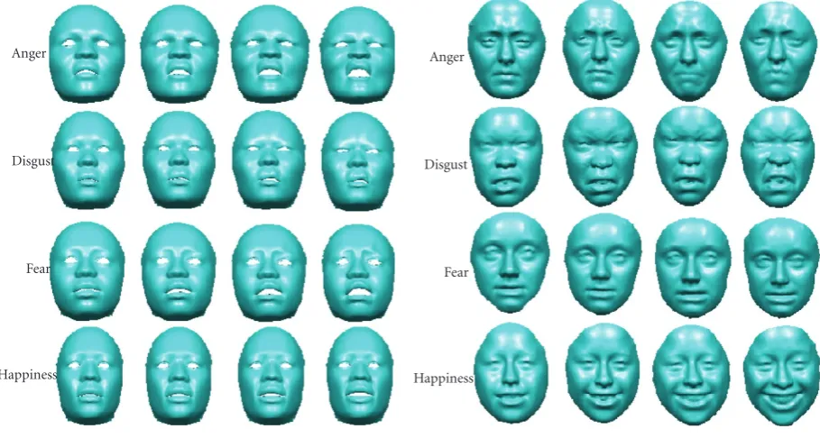
Figure4: Face samples showing four different subjects and expressions with four levels of expression intensity.
showing different individuals and different expressions are shown inFigure 4. The faces used for testing are not included in the training data sets used for building the SSM.
4.1. Qualitative Evaluation. Since the high-dimensional SSV-based features are hard to visualise, only the first three elements of the SSV are used for qualitative analysis. For different types of data, the first three principal compo-nents retain different levels of variability present in the training data set. With the retained variability defined as 3
i=1λi/
M
i=1λi, whereλiandMare given inSection 2.2, the
first three principal components retain around 51% of the total data variability for the model built using 450 synthetic faces. For the model built from the facial landmarks the first three principal components retain around 42% data shape variability, whereas for the model built using dense set of facial points the first three principal components retain 35% of the variability. The last two models were built using the same 450 faces randomly selected from the BU-3DFE database.
4.1.1. 3-D Synthetic Faces. Firstly, the 3D synthetic faces generated from the FaceGen Modeller are used to show the separability of the SSV-based features. The FaceGen Modeller is a commercial software designed to create realistic faces with controllable type and level of expressions for subjects of any ethnic origin or gender. Since the correspondence information is provided for all the face vertices (3428 vertices are used to represent all the synthetic faces), the SSM can be built directly without correspondence search. However, it needs to be stressed that the priori knowledge about the correspondence, for the faces in the training data set,
was only used in the model building stage. In the model fitting stage the information about the data correspondence was ignored and the correspondence search was included in finding the SSV representation of the faces from the test sets. For the evaluation, a training data set of 450 3D synthetic faces from 18 subjects was used to build the SSM. A sample of faces from the training data set is shown in Figure 4(a). Another 450 synthetic faces of 18 subjects were used for testing. The training and testing faces are mutually exclusive. First, for clarity of the presentation,Figure 5shows the separability of the synthetic faces’ SSVs for selected expression pairs with five different subjects and varying expression’s intensity. The SSVs of the same subject and representing the same expression with various expression’s intensity are linked together. Considering the expression’s intensity as only variable the corresponding SSVs are aligned on the same line segment. It can be observed that the SSV-based features corresponding to different subjects and different facial expressions are well separated; furthermore the orientation of each line seems to define a type of the expression.Figure 6shows the separability of the synthetic faces’ SSVs for all six basic expressions and five subjects shown in different colours. It can be seen that the SSVs representing different expressions for the same subject are clustered together and the SSVs representing the same expression are located on the line segments having the same orientation which is independent of the subject.
20 40 60 80 100 120
b3
50 0
−50 −100
−150
b2
−150 −100
−50 0 50
b1 Happiness
Sadness
(a) Happiness versus Sadness
20 40 60 80 100 120
b3
50 0
−50 −100
−150
b2
−150 −100
−50 0 50
b1 Anger
Disgust
(b) Anger versus Disgust
20 40 60 80 100 120
b3
50 0
−50 −100
−150
b2
−150 −100
−50 0 50
b1 Anger
Fear
(c) Anger versus Fear
Figure5: Visualization of the synthetic faces separability using first three elements of the SSV and five different subjects.
for face generation was previously proposed in computer graphics literature [35]. From the presented results, it can be concluded that the proposed face registration method is able to recover the facial expression and subject con-trol parameters used in the face generation model (e.g., orientations of the clustered lines in the SSV space define
−200 −150 −100 −50 0 50 100
b3
300 200
100 0
−100−200
b2 200 100
0 −100
−200−300
b1
Anger Disgust Fear
Happiness Sadness Surprise
Figure6: Visualization of the synthetic faces separability for six expressions and five subjects.
(a) Neutral. (b) Surprise.
Figure7: Example of manually selected landmarks in two different faces from the BU-3DFE database.
eigen faces responsible for generating different expressions in the FaceGen shape space model, whereas positions of the clustered lines define the subject’s identity, as shown in Figures5and6).
−20 −15 −10 −5 0 5 10 15 20
b3
−40 −20
0 20
40
b2
−60 −40 −20 0
20 40
b1
Happiness Sadness
(a) Happy versus sad
−20 −10 0 10 20 30
b3
40 20
0 −20
−40
b2 −80−60
−40−20 0 20
40
b1
Anger Disgust
(b) Angry versus disgust
−30 −20 −10 0 10 20 30
b3
−40 −20
0 20
40
b2
−40
−20 0 20
40
b1
Anger Fear
(c) Angry versus fear
Figure 8: Separability analysis for manually selected landmarks using first three principal components.
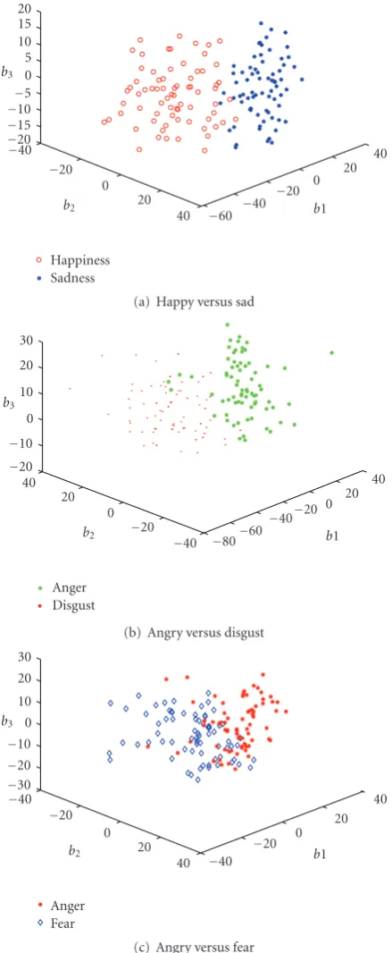
Figure 8demonstrates the separability of the SSV feature space, derived using manually selected landmarks. The first three elements of the SSV were used with five types of facial expressions. Figure 8(a)shows that facial expressions of happy and sad can be easily separated even in a low-dimensional SSV feature space. This is in agreement with the general consensus that the expressions of sadness and
happiness are the most recognisable human expressions as confirmed by a number of psychophysical test. Some of the expressions are not as well separated in the feature space as, for example, “angry” and “fear”, as shown in Figure 8(c). Although they are partly “mixed” together in the low-dimensional shape space, it is still possible to separate the majority of these facial expressions. Again this result reflects findings of psychophysical tests, which confirm that expressions such as anger and fear can be easily misclassified by a human observer [36].
4.1.3. Full 3D Face Scans. The results from the previous section show that with the use of the SSV feature space it is possible to discriminate facial expressions on real facial scans. Unfortunately, although the SSM built from manually selected landmarks uses real faces, the correspondence is established manually. This approach would not be a satisfactory solution for most applications as the manual landmark selection is too tedious and time consuming. In this section discriminatory characteristics of the SSV feature space constructed using a dense set of facial points, as described inSection 3, are examined. As explained there, the correspondence is estimated automatically during the pose estimation stage of the model fitting process. It should be noted here that as the dense correspondence is not given in the training data set, the correspondence between points on different training facial scans is also estimated during the model building phase as explained inSection 2.1.
Figure 9 illustrates the separability of the facial expres-sions in the feature space of the first three principal components of the SSV built from the full facial scans. As in the previous section five different facial expressions were used. Similarly to the results shown for the manually selected facial landmarks the results demonstrate again that the SSV feature space offers a good expression separability.
4.1.4. Automatically Selected Facial Landmarks. As shown in the previous section, the SSV feature space built from full facial scans, using dense facial points, provides good separability of expressions. Additionally this approach is more practical as the correspondence is estimated auto-matically. Intuitively discriminatory characteristics of the SSV feature space can be further improved by using only information from the facial regions which are articulated the most during different expressions. In the “full facial scan” approach, all the points contribute to the SSM, but some points, that is, on a forehead, carry very little information about face expression. These points would still contribute to the variations of the SSM model as they would represent variability of facial shape for different subjects. Evaluation was therefore carried out to use the “full facial scan” SSM first to establish the correspondence between the model and the data and subsequently used the SSM built from predefined facial landmarks on the model for the facial expression representation.
−400 −300 −200 −100 0 100 200 300 400
b3
−500
0
500
b2
−400
−200 0 200
400
b1
Happiness Sadness
(a) Happy versus sad
−400 −300 −200 −100 0 100 200 300 400
b3
400 200
0 −200
−400
b2
−1000 −500 0
500 1000
b1
Anger Disgust
(b) Angry versus disgust
−600 −400 −200 0 200 400
b3
−500 0
500 1000
b2 −400 −200
0 200
400
b1
Anger Fear
(c) Angry versus fear
Figure9: Separability of the facial expressions in the feature space of first three principal components of the SSV built from the full facial scans.
is automated, where the automation is achieved through registration of the “full facial scan” SSM with a new face. Since the corresponding indices of the facial landmarks on the model are already known, the positions of the corresponding landmarks on a new face scan can be directly estimated when the model is matched to the new face scan. In this case the surface registration error may introduce
variability in the position of the landmarks which in turn may have negative effects on the classification performance. To examine registration accuracy of the proposed method tests were carried with the synthetic and real faces. In the experiments, for each data type, the model has been matched to 450 faces which were not used for the model building. Subsequently the Euclidean distance between corresponding landmarks on the deformed model and the test faces was calculated. The average distance between corresponding landmarks on the synthetic faces and the model, calculated from all the 450 test faces, was 1.49 mm with maximum error of 3.95 mm, whereas corresponding distances obtained for the real faces were 3.56 mm and 7.64 mm, respectively. The bigger registration errors obtained for the real faces are mainly thought to be due to the errors in the manual selection of the facial landmarks. Indeed it is believed that the errors in the manual landmark selection, used in the model building stage, have more influence on the method performance than the registration error.
Similar to the previous experiments, the model is built using 450 face scans from 18 randomly selected subjects, and another 450 face scans from 18 subjects are used for testing.Figure 10shows the separability test for the proposed method. As before the first three principal components are used to represent five facial expressions. Compared to the case with the manually selected facial landmarks, the SSV feature space offers a comparable performance on separability of expressions.
4.2. Quantitative Evaluation. The separability of the SSV-based features has been demonstrated qualitatively in the preceding section. This qualitative analysis shows that the SSV feature space exhibits good facial expressions separabil-ity. Due to the way the synthetic data is generated, the SSV-based features in that case were seen to form very distinctive linear patterns with different line directions responsible for different expressions. From experiments with real facial scans from the BU-3DFE database, the best performance is achieved when landmarks are used to build the SSM.
In order to further investigate the separability of the SSV-based features, a quantitative evaluation was carried out. For this analysis, only the SSM which was generated using the data from the real scans was included in the test. The data sets included (i) manually selected facial landmarks, (ii) full face scans, and (iii) automatically selected facial landmarks. In this quantitative evaluation, a computable criterion based on the within-class and between-class distances [37] was used to measure the separability of expressions in the corresponding SSV feature spaces. A similar criterion has been used by Wang and Yin [8] to evaluate the separability of topographic context (TC) and intensity-based features for the facial expression analysis and recognition. The criterion relies on the average between-class distance in the case of multiple categories, which is defined as follows:
J1(x)=1
2
Nc
i=1
Pi Nc
j=1
Pj
1
MiMj Mi
k=1
Mj
l=1
−30 −20 −10 0 10 20
b3
−60 −40
−20 0
20 40
b2 −40 −20
0 20
40
b1
Happiness Sadness
(a) Happy versus sad
−30 −20 −10 0 10 20 30
b3
40 20
0 −20
−40
b2
40 20 0
−20 − 40
b1
Anger Disgust
(b) Angry versus disgust
−30 −20 −10 0 10 20 30
b3
−40 −20
0 20
40
b2 −40
−20 0 20
40
b1
Anger Fear
(c) Angry versus fear
Figure 10: Separability analysis for automatically selected land-marks using first three principal components.
whereMiandMjare the number of samples in classesμi, and
μj,xik, andx j
l are theK-dimensional feature vectors (SSV)
with labelsμi andμj.Nc is the number of distinct classes.
Pi and Pj are the class-prior probabilities, and δ(xki,x j l)
denotes the distance between two samples, which is usually
calculated using Euclidean distance.J1(x) can be represented in a compact form by using the so-called within-class scatter matrixSW and between-class scatter matrixSB [38], which
are defined as follows:
SW = Nc
i=1
Pi 1
Mi Mi
k=1
xki−mi
xik−mi
T
,
SB= Nc
i=1
Pi(mi−m)(mi−m)T,
(38)
wheremiis the mean of samples in theith class:
mi= 1
Mi Mi
k=1
xik, (39)
andmis the mean for all of the samples:
m=
Nc
i=1
Pimi. (40)
Using (38),J1(x) can be rewritten in the following form:
J1(x)=tr(SW+SB). (41)
AlthoughJ1(x) is an efficient and computable separability criterion for feature selection, it is not appropriate for comparing two or more features since the calculated value of
J1(x) depends on the scale and dimensionality of the feature space. In order to compare two or more features which lie in different spaces with different scales and dimensionalities, a new criterion,J2(x), similar toJ1(x), is used (as in [8]) based on a natural logarithm of the ratio of the determinant of the within-class scatter matrix and between-class scatter matrix. The new metric is defined as
J2(x)=ln|(SW+SB)|
smax
, (42)
wheresmaxis the entry which contains the maximum value in matrixΣ, and matrixΣis obtained using the singular value decomposition (SVD) of matrixSW:
SW =UΣVT. (43)
Table1: Recognition rate.
Feature type/classifier LDA (%±SD) QDC (%±SD) NNC (%±SD)
Synthetic faces 98.00±1.33 100.00±0.00 70.89±2.52
Real faces 81.89±6.96 80.11±6.87 79.00±7.09
Manually selected landmarks 84.67±4.12 82.44±5.48 83.22±6.42
Automatically selected landmarks 82.78±4.64 80.34±5.03 81.78±5.28
SD: Standard Deviation.
0 10 20 30 40 50 60 70
J2
(
x
)
0.4 0.5 0.6 0.7 0.8 0.9 1 Energy retained
Manually selected facial landmarks Automatically selected facial landmarks Full facial scans
Figure11: Quantitative evaluation of facial expression separability in the SSV feature spaces.
Table2: Confusion matrix of the LDA classifier for the synthetic faces.
Input/output Anger Disgust Fear Happy Sad Surprise
(%) (%) (%) (%) (%) (%)
Anger 94.00 2.00 2.00 2.00 0.00 0.00
Disgust 0.00 100.00 0.00 0.00 0.00 0.00
Fear 0.00 2.00 98.00 0.00 0.00 0.00
Happy 0.00 0.00 0.00 96.00 2.00 2.00
Sad 0.00 0.00 0.00 0.00 100.00 0.00
Surprise 0.00 0.00 0.00 0.00 0.00 100.00
5. Experiments on Facial
Expression Recognition
The separability analyses performed in the previous section indicate that the SSV feature space can be used in principle for classification of facial expressions. In this section, the person-independent facial expression recognition experi-ments using the high-dimensional SSV are conducted to further validate discriminatory properties of the SSV feature space. Again, four different types of facial data were used in the experiments. For each type of facial data, 900 faces from
Table3: Confusion matrix of the LDA classifier the real faces.
Input/output Anger Disgust Fear Happy Sad Surprise
(%) (%) (%) (%) (%) (%)
Anger 82.64 3.48 4.17 3.47 4.86 1.39
Disgust 7.64 78.47 3.48 5.56 2.08 2.78
Fear 4.17 3.47 72.59 12.50 5.56 1.39
Happy 2.78 5.56 8.33 83.33 0.00 0.00
Sad 4.17 3.47 11.11 0.00 81.25 0.00
Surprise 0.00 0.00 4.17 2.78 0.00 93.06
Table4: Confusion matrix of the LDA classifier for the manually selected landmarks.
Input/output Anger Disgust Fear Happy Sad Surprise
(%) (%) (%) (%) (%) (%)
Anger 90.97 4.17 0.00 0.00 4.86 0.00
Disgust 2.08 89.58 2.78 3.47 0.69 1.39
Fear 0.00 4.86 70.14 4.86 14.58 5.56
Happy 1.38 3.47 6.94 88.19 0.00 0.00
Sad 9.72 0.00 11.81 5.56 72.92 0.00
Surprise 2.08 0.00 1.39 0.00 0.00 96.52
Table5: Confusion matrix of the LDA classifier for the automati-cally selected landmarks.
Input/output Anger Disgust Fear Happy Sad Surprise
(%) (%) (%) (%) (%) (%)
Anger 90.28 0.00 2.08 3.47 4.17 0.00
Disgust 4.16 81.94 4.16 2.78 1.40 5.56
Fear 2.78 4.16 65.97 8.18 11.81 5.56
Happy 5.56 0.00 6.94 87.50 0.00 0.00
Sad 3.47 5.56 10.42 3.47 77.08 0.00
Surprise 2.08 0.00 3.47 0.00 0.00 94.44
Table6: Confidence confusion matrix for the human observers using 2D video sequences.
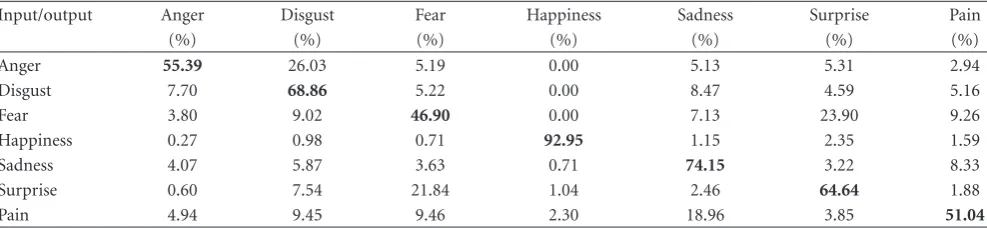
Input/output Anger Disgust Fear Happiness Sadness Surprise Pain
(%) (%) (%) (%) (%) (%) (%)
Anger 55.39 26.03 5.19 0.00 5.13 5.31 2.94
Disgust 7.70 68.86 5.22 0.00 8.47 4.59 5.16
Fear 3.80 9.02 46.90 0.00 7.13 23.90 9.26
Happiness 0.27 0.98 0.71 92.95 1.15 2.35 1.59
Sadness 4.07 5.87 3.63 0.71 74.15 3.22 8.33
Surprise 0.60 7.54 21.84 1.04 2.46 64.64 1.88
Pain 4.94 9.45 9.46 2.30 18.96 3.85 51.04
possible classification algorithm, three well-know (off -the-shelf) classification methods have been used, namely; linear discriminant analysis (LDA) [39], quadratic discriminant classifier (QDC) [40], and nearest neighbor classifier (NNC) [37]. The detailed description of these methods is beyond the scope of this paper but can be found in most of the textbooks on pattern recognition. The average recognition rates as well as standard deviations, calculated from all the six experiments using different subsets of faces, for the four different types of facial data, are give inTable 1. To have a fair comparison, the size of the SSV for each data type has been selected in such a way that the retained variability in each corresponding SSM is as similar as possible. For the results presented below, SSV for the synthetic data has 27 elements corresponding to 95.31% of retained variability, SSV for the full facial scans has 39 elements corresponding to 94.77%, whereas the SSV for the facial landmarks (both manually and automatically selected landmarks are using the same model) has 18 elements corresponding to 95.12%.
As shown inTable 1, all the classifiers achieve a similar recognition rate for the same data type with the extremely hight rates achieved for the synthetic faces for all the classifiers but the NNC classifier. For the facial data from the BU-3DFE database, the manually selected landmarks’ SSVs always reach the highest recognition rate, whereas the real faces’ SSVs always achieve the lowest rate. Tables2to5show LDA classifier confusion matrices for all the different data types used in the experiments.
The presented results show that the SSV-based features can be used for recognition of facial expressions. The results for the manually selected landmarks are included only for a reference as using this data type is not practical due to lengthy process of landmarks’ selection. From the presented results it can be seen that the best recognition rate of 82.78% obtained for the automatically selected landmarks is comparable with the best recognition rate of 84.67% obtained for the manually selected landmarks. This shows that the deformable surface registration method described inSection 3is able to recover correct correspondences. An interesting insight into classification performance can be gained by looking at the confusion matrices. FromTable 5 showing the confusion matrix of the LDA classifier for the automatically selected landmarks, it can be concluded that the anger and surprise expressions are all classified with above 90% accuracy, whereas the fear expression is
only classified correctly in 65%. This can lead to the question about adequacy of the ground truth data. This is a difficult problem as the human expressions are very subjective by their nature. To demonstrate thisTable 6shows the confidence confusion matrix obtained for the human observers. This data has been obtained as a part of the project aiming to build and validate a 3D dynamic human facial expression database [41]. The specific results shown in the table are based on 10 observers asked to rank their confidence about recognising 7 facial expressions represented in 210 video clips and each video clip lasts 3 seconds. As it can be seen in the table the observers were very confident about recognising the happy expression whereas the fear expression was often confused with the surprise expression. This shows a “subjective” nature of the ground truth data. Although recognition rate of 65% for the fear expression in Table 5 seems to be quite low, when taking into account results presented inTable 6, they can be considered as reasonable.
6. Conclusions
A novel method for facial expression representation has been presented in this paper. It uses only 3D shape information, and therefore, in contrast to most of the methods using texture, our method is invariant to changes in the illumi-nation, background, and to some extent viewing angle. The proposed method assumes that the SSV efficiently encodes facial expressions, and this encoding can be separated from the SSV variations caused by observing different faces. The performed tests indeed confirmed this hypothesis showing that the proposed representation is, at least partially, invari-ant to changes of the face ethnicity, gender, or age. A number of different configurations of the SSM have been tested. These include the SSM built from facial landmarks as well as full facial scans of real as well as simulated data. A fully automatic method has also been proposed for estimation of the SSV, with an iterative procedure which in turn estimates correspondence and shape parameters.
7. Future Work
(a) Texture
(b) Shape
Figure12: An example of the dynamic 3D face sequence.
−20 −10 0 10 20
b3
40 20
0 −20
−40 −60
b2
0 −10
−20 − 30−
40 −50
b1
Anger Fear
Figure13: Trajectories of the first three principal components of the SSV-based feature on dynamic face sequences.
would include construction of a hierarchical system, where firstly the face type is decided upon, and subsequently the facial expression is recognized using shape model built from the facial expression database constructed for that specific face type detected in the previous step.
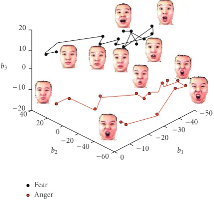
The separability results presented in the paper show that the SSV feature space can offer generally good separation for different expressions. For some expressions though such as angry and fear, the method provides only a limited separation, at least for the data used in the experiments. As a result, these expressions can be easily confused. One way to improve the separation of these “difficult” expressions is to provide more information to the model. From the reported psychophysical test it can be concluded that temporal infor-mation of the expression articulation provides important cues for human observers and helps them to correctly read expressions. Following this observation some simple tests were conducted with dynamic 3D facial scans. The dynamic face sequences are captured by the 3dMD scanner [42] in
ADSIP research centre, and the facial landmarks set on each face in the sequence were manually labeled subsequently. An example of face sequence is shown in Figure 12. Using the face sequences, the trajectory of each specified facial expression is recorded and displayed in the 3D feature space. Figure 13shows two trajectories plotted in the SSV domain for sequences representing fear and angry expressions. It can be seen that these trajectories are well separated in the SSV domain, thereby illustrating the potential usefulness of the temporal information of the face articulation for automatic expression classification.
Acknowledgments
The authors would like to acknowledge Dr. Lijun Yin from Binghamtopn University (USA) for making available to them BU-3DFED database. This work has been supported in part by the MEGURATH project (EPSRC grant no. EP/D077540/1).
References
[1] L. Yin, X. Wei, P. Longo, and A. Bhuvanesh, “Analyzing facial expressions using intensity-variant 3D data for human computer interaction,” inProceedings of the 18th International Conference on Pattern Recognition (ICPR ’06), pp. 1248–1251, 2006.
[2] P. Eisert and B. Girod, “Analyzing facial expressions for virtual conferencing,”IEEE Computer Graphics and Applications, vol. 18, no. 5, pp. 70–78, 1998.
[3] C. L. Lisetti and D. J. Schiano, “Automatic facial expression interpretation: where human-computer interaction, artificial intelligence and cognitive science intersect,”Pragmatics and Cognition, vol. 8, no. 1, pp. 185–235, 2000.
[4] S. Brahnam, C.-F. Chuang, F. Y. Shih, and M. R. Slack, “Machine recognition and representation of neonatal facial displays of acute pain,”Artificial Intelligence in Medicine, vol. 36, no. 3, pp. 211–222, 2006.
[5] S. D. Pollak and P. Sinha, “Effects of early experience on children’s recognition of facial displays of emotion,” Develop-mental Psychology, vol. 38, no. 5, pp. 784–791, 2002.
[6] E. Vural, M. Cetin, A. Ercil, G. Littlewort, M. Bartlett, and J. Movellan, “Drowsy driver detection through facial movement analysis,” inProceedings of the IEEE International Workshop on Human Computer Interaction (HCI ’07), vol. 4796 ofLecture Notes in Computer Science, pp. 6–18, October 2007.
[7] B. Fasel and J. Luettin, “Automatic facial expression analysis: a survey,”Pattern Recognition, vol. 36, no. 1, pp. 259–275, 2003. [8] J. Wang and L. Yin, “Static topographic modeling for facial expression recognition and analysis,” Computer Vision and Image Understanding, vol. 108, no. 1-2, pp. 19–34, 2007. [9] J. Wang, L. Yin, X. Wei, and Y. Sun, “3D facial expression
recognition based on primitive surface feature distribution,” in
Proceedings of the IEEE International Conference on Computer Vision and Pattern Recognition (CVPR ’06), pp. 17–26, 2006. [10] Y. Huang, Y. Wang, and T. Tan, “Combining statistics of
geometrical and correlative features for 3D face recognition,” inProceedings of the British Machine Vision Conference, pp. 879–888, 2006.
[12] V. Blanz and T. Vetter, “Face recognition based on fitting a 3D morphable model,”IEEE Transactions on Pattern Analysis and Machine Intelligence, vol. 25, no. 9, pp. 1063–1074, 2003. [13] M. Hoch, G. Fleischmann, and B. Girod, “Modeling and
animation of facial expressions based on B-splines,”The Visual Computer, vol. 11, pp. 87–95, 1994.
[14] P. Ekman and W. Friesen,The Facial Action Coding System: A Technique for the Measurement of Facial Movement, Consulting Psychologists Press, 1978.
[15] A. Saxena, A. Anand, and A. Mukerjee, “Robust facial expres-sion recognition using spatially localized geometric model,” in Proceedings of the International Conference on Systemics, Cybernetics and Informatics, pp. 124–129, 2004.
[16] M. J. Black and Y. Yacoob, “Recognizing facial expressions in image sequences using local parameterized models of image motion,”International Journal of Computer Vision, vol. 25, no. 1, pp. 23–48, 1997.
[17] H. Kobayashi and F. Hara, “Facial interaction between ani-mated 3D face robot and human beings,” in Proceedings of the IEEE International Conference on Systems, Man and Cybernetics, vol. 4, pp. 3732–3737, 1997.
[18] W. Quan, B. J. Matuszewski, L.-K. Shark, and D. Ait-Boudaoud, “Low dimensional surface parameterisation with applications in biometrics,” inProceedings of the 4th Interna-tional Conference Medical Information Visualisation: BioMedi-cal Visualisation (MediViz ’07), pp. 15–22, 2007.
[19] W. Quan, B. J. Matuszewski, L.-K. Shark, and D. Ait-Boudaoud, “3-D facial expression representation using B-spline statistical shape model,” inProceedings of the Vision, Video and Graphics Workshop, 2007.
[20] W. Quan, B. J. Matuszewski, L.-K. Shark, and D. Ait-Boudaoud, “3-D facial expression representation using statis-tical shape model,” inProceedings of the BMVA Symposium on 3D Video—Anaysis, Display and Application, 2008.
[21] H. B. J¨ahne and F. Haußecker,Computer Vision and Applica-tions, Academic Press, New York, NY, USA, 2000.
[22] FaceGen Modeller, “Singular Inversions,” 2003, http:// www.facegen.com/.
[23] L. Yin, X. Wei, Y. Sun, J. Wang, and M. J. Rosato, “A 3D facial expression database for facial behavior research,” in
Proceedings of the 7th International Conference on Automatic Face and Gesture Recognition (FGR ’06), vol. 2006, pp. 211– 216, 2006.
[24] T. F. Cootes, C. J. Taylor, D. H. Cooper, and J. Graham, “Active shape models-their training and application,”Computer Vision and Image Understanding, vol. 61, no. 1, pp. 38–59, 1995. [25] X. Lu and A. K. Jain, “Deformation modeling for robust
3D face matching,” inProceedings of the IEEE International Conference on Computer Vision and Pattern Recognition (CVPR ’06), vol. 2, pp. 1377–1383, 2006.
[26] F. L. Bookstein, “Principal warps: thin-plate splines and the decomposition of deformations,”IEEE Transactions on Pattern Analysis and Machine Intelligence, vol. 11, no. 6, pp. 567–585, 1989.
[27] X. Lu and A. K. Jain, “Deformation analysis for 3D face matching,” in Proceedings of the 7th IEEE Workshop on Applications of Computer Vision (WACV/MOTIONS ’05), vol. 1, pp. 99–104, 2005.
[28] K. Rohr, H. S. Stiehl, R. Sprengel, et al., “Point-based elastic registration of medical image data using approximating thin-plate splines,” inProceedings of the 4th International Conference on Visualization in Biomedical Computing, pp. 297–306, 1996.
[29] J. Peters and U. Reif, “The simplest subdivision scheme for smoothing polyhedra,”ACM Transactions on Graphics, vol. 16, no. 4, pp. 420–431, 1997.
[30] A. Blake and M. Isard, Active Contours, Springer, Berlin, Germany, 1998.
[31] T. Vrtovec, D. Tomazevic, B. Likar, L. Travnik, and F. Pernus, “Automated construction of 3D statistical shape models,”
Image Analysis and Stereology, vol. 23, pp. 111–120, 2004. [32] P. J. Besl and N. D. McKay, “A method for registration of
3-D shapes,”IEEE Transactions on Pattern Analysis and Machine Intelligence, vol. 14, no. 2, pp. 239–256, 1992.
[33] K. S. Arun and T. S. Huang, “Least-square fitting of two 3-D point sets,”IEEE Transactions on Visualization and Computer Graphics, vol. 9, no. 5, pp. 698–700, 1987.
[34] S. Umeyama, “Least-squares estimation of transformation parameters between two point patterns,”IEEE Transactions on Pattern Analysis and Machine Intelligence, vol. 13, no. 4, pp. 376–380, 1991.
[35] J. Ahlberg, “CANDIDE-3—an updated parameterized face,” Tech. Rep. LiTH-ISY-R-2326, Image Coding Group, Depart-ment of EE, Link¨oping University, Link¨oping, Sweden, Jan-uary 2001.
[36] P. Ekman and W. V. Friesen, “Constants across cultures in the face and emotion,”Journal of Personality and Social Psychology, vol. 17, no. 2, pp. 124–129, 1971.
[37] R. O. Duda, P. E. Hart, and D. G. Stork,Pattern Classification, John Wiley & Sons, New York, NY, USA, 2nd edition, 2001. [38] W. Zhao, R. Chellappa, and A. Krishnaswamy, “Discriminant
analysis of principal components for face recognition,” in
Proceedings of the 3rd International Conference on Face & Gesture Recognition, pp. 336–341, 1998.
[39] P. McCullagh and J. A. Nelder, Generalized Linear Models, Chapman and Hall, New York, NY, USA, 2nd edition, 1989. [40] B. D. Ripley,Pattern Recogntion and Neural Networks,
Cam-bridge University Press, CamCam-bridge, UK, 1996.
[41] B. J. Matuszewski, C. Frowd, and L. K. Shark, “Dynamic 3D facial database,” Faculty of Science and Technology, University of Central Lancashire, 2008.