Volume 2009, Article ID 421540,11pages doi:10.1155/2009/421540
Research Article
Rate-Optimal and Reduced-Complexity Sequential Sensing
Algorithms for Cognitive OFDM Radios
Seung-Jun Kim and Georgios B. Giannakis
Department of Electrical and Computer Engineering, University of Minnesota, 200 Union Street SE, Minneapolis, MN 55455, USA
Correspondence should be addressed to Georgios B. Giannakis,[email protected] Received 19 February 2009; Revised 22 May 2009; Accepted 14 July 2009
Recommended by Ananthram Swami
Sequential sensing algorithms are developed for OFDM-based hierarchical cognitive radio (CR) systems. Secondary users sense multiple subbands simultaneously for possible spectrum availabilities under hard misdetection constraints to prevent interference to the primary users. Accounting for the fact that the sensing time overhead can often be significant, a novel performance metric is introduced based on the effective achievable data rate. An optimization problem is formulated in the framework of optimal stopping problems to maximize the average effective data rate by determining the best time to stop taking samples and proceed to data transmission. A basis expansion-based suboptimal algorithm is developed to reduce the prohibitive complexity of the optimal solution. The numerical results presented verify the efficacy of the proposed approach.
Copyright © 2009 S.-J. Kim and G. B. Giannakis. This is an open access article distributed under the Creative Commons Attribution License, which permits unrestricted use, distribution, and reproduction in any medium, provided the original work is properly cited.
1. Introduction
The cognitive radio (CR) paradigm aims to design intelligent radios that can sense the environment and adapt the transceiver parameters as well as the resource allocation deci-sions in order to exploit the spectrum availability aggressively [1]. The motivation stems from the observation that the current usage pattern of the licensed spectrum is not very efficient; there are plenty of “white spaces” in spectral and/or spatiotemporal domains that allow overlaying secondary transmissions on top of the existing licensed (a.k.a. primary) users without degrading the communication quality of the latter [2].
To exploit the spectrum holes opportunistically, orthog-onal frequency-division multiplexing (OFDM) transceivers are often employed at the physical layer of the CR due to their flexibility in communicating over a wide range of spectrum bands efficiently [3]. OFDM radios can easily implement transmission filters that suppress the signal in the undesired subbands to prevent interference to the primary users (PUs). CR transmissions target only the bands in which the PUs are not present. In the time domain, the “quiet” periods of the PUs are identified so as to interleave the CR data in-between the PU transmissions [4].
Obviously, a key component of CR transceivers is the sensing module that monitors spectrum occupancy of the PUs in real time. Since the presence of CR links must be oblivious to the PUs, hard misdetection constraints need be imposed to the design of the detector in the sensing module. However, this inevitably leads to increased sensing time, which, in turn, leaves less time for the actual data transmission before the PUs may kick back in. Thus, it is important to factor in the sensing overhead in the design of the sensing module, especially for scenarios where the PU occupancy changes dynamically in time as well as in frequency.
also performance such as energy detectors [6,7] or feature-based detectors [8].
The wideband sensing problem for OFDM-based CRs was considered in [9], where the detection thresholds for a bank of energy detectors were optimized jointly to maximize throughput performance. To improve the sensing perfor-mance, cooperative sensing scenarios were also considered in [10] by collecting measurements from multiple CRs at the fusion center (FC) to improve detection performance. A cooperative sensing strategy was also pursued in [11], where a linear-quadratic fusion rule was developed based on the deflection criterion to process correlated observations. The tradeoff between sensing duration and throughput was studied in [12] using the energy detectors. These developments, however, assume batch (or fixed sample size (FSS)) detection strategies, where the number of samples collected for detection is a predetermined design parameter, which does not depend on the actual values of the received samples.
Sequential detection schemes on the other hand exploit the fact that the number of samples required to achieve a given reliability level may well be dependent on the actual realization of the observed samples. For example, in a simple binary hypothesis testing context, Wald’s sequential probability ratio test (SPRT) compares the likelihood ratio with two thresholds, and the decision is made as soon as the test statistic exceeds either one of the thresholds. It is known that SPRT minimizes the average sample number (ASN) among all tests with the same false alarm and misdetection probabilities [13, page 21]. However, it is not clear how to apply the SPRT approach to the wideband sensing problem, where a bank of detectors must be run simultaneously. Moreover, the relevant optimization criterion in this case might not be as simple as the ASN. In [14], two layers of SPRTs were employed at individual CRs and the FC to reduce the overall detection delay for a single-channel sensing problem. However, no claims on optimality were provided.
In this work, rate-optimal wideband sequential sensing algorithms are developed in the framework of optimal stopping time problems. Such problems amount to deter-mining the time to stop taking sequential observations so that an expected value of payoffbased on the accumulated observations is maximized [15,16]. The payoffin our CR sensing setup will be chosen as the total rate achieved by using all the available subchannels, where the availability is determined under hard interference constraints. The sensing overhead is captured by explicitly accounting for the sensing time, which consumes portion of the frame duration.
In a companion paper [17], generalizations to sequential
cooperative sensing are also discussed, where a central processing unit sequentially collects either raw (analog) or quantized observations from multiple cooperating CRs. However, the underlying problem formulation is different in [17] in that the detector structure is optimally determined in closed form as a likelihood ratio test, whereas the conventional energy detector structure is adopted here. Also, arecursive(on-line) counterpart of thebatchtraining algorithm developed here is presented in [17].
The rest of the paper is organized as follows. InSection 2, the signal model and the problem formulation are presented for the single-CR case. InSection 3, the optimal solution is derived and a reduced-dimension sufficient statistic is iden-tified.Section 4develops a basis expansion-based reduced-complexity algorithm to obtain a suboptimal yet tractable solution. Numerical results are presented inSection 5, and conclusions are provided inSection 6.
2. Problem Statement
2.1. Signal Model. Consider a CR that sharesMorthogonal bands opportunistically with PUs in its network. In order not to interfere with on-going PU transmissions, the CR must identify the bands that are not occupied by the PUs before transmitting its own data.
Thenth received signal sample at the CR on bandm ∈ {1, 2,. . .,M}, when a PU is transmitting on that band, can be modeled by
rn(m)=h(nm)sn(m)+zn(m), n∈ {1, 2,. . .,N}, (1)
where {h(nm)} are the channel coefficients, {s(nm)} are the PU signal samples, {zn(m)} are independent and identically distributed (i.i.d.) complex Gaussian additive noise samples with mean 0 and varianceσ2, andNdenotes the maximum
number of samples that can be collected in the sensing phase. Under the assumption that PU occupancy is independent across the M bands, the CR must perform a binary hypothesis test per bandmto discriminate the following two hypotheses:
H0(m):r(nm)=z(nm), n∈ {1,. . .,N},
H1(m):r(nm)=h(nm)sn(m)+z(nm), n∈ {1,. . .,N}. (2)
The prior probabilities Pr{H0(m)}and Pr{H(
m)
1 }are denoted
byp(0m)and 1−p (m)
0 , respectively.
As in, for example, [6], each CR receiver relies on energy detection to decide the occupancy of each band. The test statistictn(m)is calculated at each time stepnas
t(m)
n = n
k=1
yk(m), yn(m)rn(m)
2
. (3)
For simplicity, assume that the channel coefficients{h(nm)} do not vary over the detection interval such that|h(nm)|2can be denoted asG(m),∀n ∈ {1,. . .,N}, and the transmitted
signal has unit power; that is, E{|s(nm)|2} = 1, ∀n,m. The CR receiver in the scenarios considered can acquire its channel with the PU blindly, or, by overhearing the pilot signal transmitted by the PU system. This is clearly feasible when the transceivers are stationary so that the channel is quasistatic; see also [9] for a justifying argument in the context of DTV systems. In addition, it is possible to extend the ensuing formulation and algorithms to the case where only the distribution ofG(m)is known by considering
case goes beyond the scope of the present paper and will not be detailed here.
Then, the observations {y(1m),y2(m),. . .,y(Nm)} are i.i.d. under H0(m) and H1(m) with the conditional univariate
densities under the two hypotheses for all mgiven by the (non)centralχ2densities [18, Section 2.2]:
py|H0(m)
= 1 σ2e
−y/σ2
1{y≥0}, (4)
py|H1(m)
= 1 σ2e
−(y+G(m))/σ2 I0
⎛ ⎝
G(m)y
σ2/2
⎞
⎠, (5)
whereI0(·) denotes the zeroth-order-modified Bessel
func-tion of the first kind, and1{·} the indicator function that
equals 1 if the condition{·}is true and 0 otherwise.
In the batch Neyman-Pearson framework, the decision with maximum detection probability under a given false-alarm rate is based on the threshold rule
DecideH1(m) iftn(m)> γ(nm),
DecideH0(m) iftn(m)< γ(nm)
(6)
due to the monotonicity of the log-likelihood ratio, where γn(m)is the threshold at timenfor bandm, and the decision can be either way when t(nm) = γn(m). Invoking the central limit theorem, one can show that for large enough n the probability of false alarms α(nm) and the probability of misdetectionβ(nm) for bandmwith sample sizenare given by [19]
α(m)
n =Pr
t(m)
n > γ(nm)|H
(m) 0
=Q
⎛
⎝γ(nm)−nσ2 σ2√n
⎞
⎠, (7)
β(m)
n =Pr
t(m)
n < γ(nm)|H
(m) 1
=1−Q
⎛ ⎝γ
(m)
n −n
σ2+G(m)
σ
n(σ2+ 2G(m))
⎞
⎠, (8)
whereQ(·) denotes the Gaussian tail function.
In the context of spectrum sensing for CRs, the mis-detection probabilities signify the probabilities of failing to detect the presence of the PUs, which could lead to causing interference to the PU transmission. For this reason, the sensing algorithms must be designed to guarantee very small misdetection probabilities. On the other hand, small false alarm probabilities are desired to increase the usage of the available channels. These dual goals can be accomplished by increasing the sample size n. However, increasing the sample size leads to larger sensing overhead, which effectively reduces the time left for actual data transmission. In the next subsection, a sequential sensing problem is formulated to optimize the overall transmission rate by taking into account the overhead due to sensing.
2.2. Sequential CR Sensing as an Optimal Stopping Problem.
The sequential sensing problem can be formulated in the
Sensing phase Band 1 Band 2
BandM
Frame durationT
Ts
nTs
Data transmission phase
· · ·
· · · · · ·
. . .
. . .
. . .
Figure1: Frame structure of the CR.
framework of optimal stopping problems [20, Section 4.4], [15, 16, 21]. Based on the observations collected up to a certain point, the optimal stopping problems seek to find the “best” time to stop taking observations, “best” in the sense of maximizing the expected value of a chosen reward. An optimal stopping problem can thus be defined by specifying (i) a sequence of observed random variables with their joint distribution and (ii) a sequence of random variables, whose joint distributions with the observations are known, each representing the per-step reward that could be obtained should one decide to stop at the corresponding time step. In our setup, the sequence of i.i.d. observations is{yn}Nn=1,
whose joint p.d.f. is expressible in terms of the univariate p.d.f. in (4) or (5). In the ensuing subsections, the sequential CR sensing problem is posed as an optimal stopping problem by defining the reward sequence, which will be finally given in (27). But first it is prudent to specify the optimality criterion.
2.2.1. Average Throughput Criterion. To capture the effective throughput of the CR while accounting for the sensing overhead, consider the frame structure shown in Figure 1. The deterministic frame duration T is divided into the sensing and the data transmission phases, where the dura-tions of both phases are random variables. Denote the sampling interval of the detector by Ts, where T ≥ NTs. Let yn [yn(1) yn(2) · · · y(nM)]T and likewise for the corresponding vector tn [t(1)n · · · tn(M)]T, collecting the test statistics defined in (3). The PU occupancy over the Mbands is denoted by anM×1 random vectorHwith the mth entryH(m)taking values from{H(m)
0 ,H1(m)}and the rate
that can be achieved in bandmbyR(m).
If the CR stops sensing after thenth sampling interval, the duration of the sensing phase isnTs. The CR then proceeds to data transmission on the bands that are sensed idle for the remaining part of the frame of durationT−nTs. Therefore, the overall throughput is given by
fn(H,tn)
=T−nTs T
M
m=1
R(m)1{H(m)
0 }1{t(nm)<γn(m)}, n=1, 2,. . .,N,
where the first indicator function in (9) allows rate to be transmitted over bandmonly ifH(m)is indeedH(m)
0 ; while
the second indicator function allows usage of bandmif also the energy detector correctly declaresH(m)=H(m)
0 (cf. (6)).
Note that the per-step reward fn(·) is a function of the underlying true spectrum occupancy H, which is not directly observable. It can be shown that the optimal stopping problem based on the per-step reward fn(·) is equivalent to the one based on the conditional average per-step reward E{fn(H,tn) | Yn}, n = 1, 2,. . .,N, where Yn [y1· · ·yn] and the expectation is taken over H
[21], [20, Section 5.1]. Expected values of binary random variables corresponding to the indicator functions can be replaced by probabilities; for example, E{1{H(m)
0 } | Yn} = Pr{H0(m) | y(
m) 1 ,. . .,y(
m)
n }. Hence, the conditional average per-step reward can be expressed as (cf. (9))
fn(πn,tn)Efn(H,tn)|Yn
=T−nTs T
M
m=1
R(m)π(m)
n 1{tn(m)<γ(nm)},
(10)
whereπn [πn(1)· · ·πn(M)]T denotes the belief vector with entries
π(m)
n Pr
H0(m)|y (m)
1 ,. . .,y(nm)
. (11)
Clearly, the factor (T −nTs)/T in the per-step rewards in both (9) and (10) diminishes as n approaches N, which encourages stopping as soon as possible, while collecting more samples in tncan potentially identify more available bands, as captured by the indicator functions 1{t(m)
n <γ(nm)},
leading to a tradeoff.
The goal is to obtain the average (over H and YN) throughput-optimal stopping policy that determines whether to stop sensing or not at each timen∈ {1, 2,. . .,N− 1} given the observations Yn. To be precise, let un ∈ {stop, continue} denote a control variable at time n. The stopping policyUn(·) per timenis the rule specifying the mappingYn∈(R+)nMU
n(Yn)∈ {stop, continue}. With the introduction of an auxiliary state variablexn ∈ {S,S}, where xn = S indicates the “stop” state and xn = S the “nonstop” state, the system evolution is characterized by
xn+1=
⎧ ⎨ ⎩
S, ifxn=S, orxn=/S, un=stop,
S, otherwise,
n=1, 2,. . .,N−1,
(12)
wherex1 = S. The reward function at the final stageN is
given by
fN(YN,xN)= fN(πN,tN)1{xN=/S} (13)
and at stagenby
fn(Yn,xn,un)
= fn(πn,tn)1{xn=/S,un=stop}, n=1, 2,. . .,N−1.
(14)
Note that the reward at stageNdoes not include the control variable becauseUN ≡stop since sensing must end a fortiori after N sampling intervals. The “bookkeeping” variablexn ensures that the reward fn(·) may be nonzero only upon thefirst instance ofunbeing equal to “stop”; for the rest of the time steps, fn(·) evaluates to zero due to the indicator functions in (13) and (14). (As a mnemonic for the notation used, functionals with hat (e.g., fn) depend on the control (un) and the “bookkeeping” variables (xn) as well as the rewards (e.g., fn), which are functions of the dataYnthrough
πn and tn.) Expressions (13) and (14) allow the average throughput to be expressed as thesumof the per-step rewards
R(U1,. . .,UN−1)
E
⎧ ⎨
⎩fN(YN,xN) + N−1
n=1
fn(Yn,xn,Un(Yn))
⎫ ⎬ ⎭,
(15)
where the expectation is with respect toYN.
The average throughput in (15) is to be maximized over the finite horizon comprising N sampling intervals, with respect to the stopping policy {U1,. . .,UN−1} with
Un(Yn)=un∈ {stop, continue}. Certainly, to perform this functional (i.e., variational) optimization, it is necessary to know the data p.d.f. required to evaluate the expectation in (15). The reason behind expressingRin (15) as a cumulative sum of the per-step rewards in (13) and (14) is our intention of casting the sequential CR sensing task as a dynamic programming (DP) problem, the subject discussed next.
2.2.2. Constrained Dynamic Programming Formulation.
Given the observations y1,y2,. . .,yn per time n, the CR performs hypothesis testing in each band to determine whether the band is occupied or not. When the sensing is stopped, the CR transmits on those channels that the detector determines to be unoccupied. However, it is critical to constrain the “collision” probabilityPc(m)for each channel m, which is the probability that the CR interferes with the PU transmission due to misdetection. It is thus desired for the DP formulation to be introduced later to enforce the constraints
P(m)
c ≤β, m=1, 2,. . .,M, (16)
whereβis a small positive constant.
FornonsequentialFSS tests with sample sizen, the “colli-sion” probability coincides with the misdetection probability β(nm) in (8). Thus, (16) is equivalent toβn(m) ≤ βfor allm, and the thresholdγn(m)that maximizes the probability of false alarm can be calculated from (8) as
γ(m)
n =Q−1
1−βσ
n(σ2+ 2G(m)) +nG(m)+σ2. (17)
terminate at any time n ∈ {1,. . .,N}. Hence,Pc(m) can be expressed as
P(m)
c = N
n=1
Prxn=/ S,Un=stop,t(nm)< γn(m)|H
(m) 1
, (18)
whereUN ≡stop for the fixed horizonN considered here. Using Bayes’ rule, (18) can be rewritten in terms ofβ(nm)as
P(m)
c = N
n=1
β(m)
n Pr
xn=/S,Un=stop|tn(m)< γ(nm),H
(m) 1
.
(19)
Thus, if the events {xn=/ S,Un = stop} and {t(nm) < γn(m)}were independent conditioned onH1(m)for alln, then
imposing the condition β(nm) ≤ β would be sufficient to guarantee Pc(m) ≤ β. Since this is not the case in general, capping the misdetection probability under β does not necessarily ensureP(cm)≤β.
Ideally, the optimal{γn(m)} should be obtained by for-mulating a constrained DP problem that maximizes (15) under the constraints (16), after incorporating {γn(m)} as optimization variables in addition to{Un}. The resulting DP is significantly more complex to solve because the feasible space for {γn(m)} is infinite and discretization needs to be employed for tractability. For this reason, we adopt a less ideal yet intuitive rule for determining the thresholdsγ(nm), namely using the thresholds in (17) obtained from the FSS tests. The “collision” probability will still be guaranteed by explicitly imposing the conditions (16) in the constrained DP formulation described next.
First, note that the collision probability on bandmgiven in (18) can be rewritten as
P(m)
c = N
n=1
E1{xn=/S,Un=stop,t(m)
n <γ(nm)}|H
(m) 1
=E
⎧ ⎨ ⎩
N
n=1
1{xn=/S,Un=stop,t(m)
n <γ(nm)}
1−πn(m) 1−p(0m)
⎫ ⎬ ⎭,
(20)
where in deriving the second equality we used Bayes’ rule and the facts that Pr{H1(m) | y
(m) 1 ,. . .,y
(m)
n } = 1−πn(m)and Pr{H1(m)} = 1−p
(m)
0 . To render (20) compatible with the
constrained DP formalism, define per-step costs for channel m∈ {1, 2,. . .,M}as
cN(m)(YN,xN)1{xN=/S}c(Nm)
πN(m),t
(m)
N
,
c(nm)(Yn,xn,un)1{xn=/S,un=stop}c
(m)
n
πn(m),t(nm)
,
n=1, 2,. . .,N−1, (21)
where
c(m)
n
π(m)
n ,t(nm)
1{t(m)
n <γn(m)}
1−πn(m) 1−p0(m)
, n=1, 2,. . .,N.
(22)
Then, the desired optimization problem can be formulated as a constrained DP problem given by (cf. (15) and (20)–(22))
max
{Un(Yn)}Nn=−11 E
⎧ ⎨
⎩fN(YN,xN) + N−1
n=1
fn(Yn,xn,Un(Yn))
⎫ ⎬
⎭ (23)
subject toE
⎧ ⎨
⎩c(Nm)(YN,xN) + N−1
n=1
c(m)
n (Yn,xn,Un(Yn))
⎫ ⎬ ⎭
≤β, m=1, 2,. . .,M.
(24)
One approach to solving constrained DP problems is through Lagrange relaxation [22]. Given a set of Lagrange multipliers λ [λ(1) λ(2) · · · λ(M)]T
withλ(m) ≥ 0,
m∈ {1, 2,. . .,M}, the relaxedunconstrainedDP problem to solve is
max
{Un(Yn)}Nn=−11 E
⎧ ⎨
⎩gN(YN,xN;λ) + N−1
n=1
gn(Yn,xn,Un(Yn);λ)
⎫ ⎬ ⎭,
(25)
where
gN(YN,xN;λ) fN(YN,xN)− M
m=1
λ(m)cN(m)(YN,xn),
gn(Yn,xn,un;λ) fn(Yn,xn,un)− M
m=1
λ(m)c(m)
n (Yn,xn,un),
n=1, 2,. . .,N−1. (26)
Note that this is an optimal stopping problem with observa-tion sequence{yn}N
n=1and reward sequence
gn(πn,tn;λ)
fn(πn,tn)− M
m=1
λ(m)c(nm)
πn(m),tn(m)
, n=1, 2,. . .,N.
(27)
The approaches to solve the problems (25) and (26) for a givenλare described in Sections3and4.
The Lagrange multipliersλneed to be updated to satisfy the constraints in (24). A simple approach is to use the subgradient method (see, e.g., [23, Chapter 2])
λ(m+1)=max
0,λ(m)+μP(m)
c −β
, m=1, 2,. . .,M, (28)
Remark 1. Recall that the PU occupancy was assumed independent across theM bands. In practice, the resource allocation decision of the PU system may render the spec-trum occupancy of the PU transmissions correlated across bands. In principle, it is possible to cope with correlated PU spectrum occupancy. Consider, for example, M = 2 channels, where the possible occupancy states are
H0(1),H (2) 0
,H1(1),H (2) 0
,H0(1),H (2) 1
,H1(1),H (2) 1
(29)
with an associated prior for each state. By exploiting the correlation across subchannels, the sensing performance can be improved. However, the number of states and consequently the dimension of the belief vector increase exponentially in M, rendering the complexity prohibitive. This explains why we adopted the simple assumption on the spectrum occupancy being independent across the subbands.
3. Optimal Solution
In principle, the DP problem with finite horizon given in (25) and (26) can be solved optimally via the method of backward induction [20]. It can be easily verified that the backward induction for this dynamic program leads to the backward induction of the optimal stopping problems detailed next; see also [15]. To this end, define the value function Vn(·) recursively as follows:
VN(YN;λ)=gN(πN,tN;λ), (30)
Vn(Yn;λ)=maxgn(πn,tn;λ),EVn+1
Yn,yn+1;λ
|Yn
forn=N−1,. . ., 1, 0, (31)
where f0 ≡0 is used forg0in (27). This recursive definition
specifies offline functions{Vn(·)}N−1
n=0, which will be used in
the optimal stopping policy that is implemented on-line. Equation (31) proceeds backward fromn=N−1 ton= 0 by computing the value functions Vn(·) inductively. For each stepn, this involves taking the expectation of the value function of the next stepVn+1(·) over the observation vector
yn+1 conditioned on the observation history. Supposing for
now that this expectation can be obtained, the optimal value of the objective in (25) for a given Lagrange multipliers λ is provided byV0(λ). In the following, it is understood that
the exposition is for a givenλ, andλis suppressed from the notation.
Once the value functions{Vn(Yn)}N−1
n=1 are available, the
optimal stopping rule can be applied forward in time and is given by [15]
Un(Yn)=
⎧ ⎨ ⎩
stop, ifVn(Yn)=gn(πn,tn),
continue, otherwise,
n=1, 2,. . .,N−1. (32)
In practice, carrying out the backward induction is not computationally tractable. An immediate obstacle is that
one has to deal with the state vectorYn, whose dimension increases over time. Thus, it is desirable to find a statistic with lower dimensionality that is still sufficient for finding the optimal control policy. The following proposition identifies such a sufficient statistic for the problem at hand.
Proposition 1. The vectorψn[πntn]is a sufficient statistic for obtaining the optimal stopping policy.
Proof. Note first thatπn+1andtn+1can be updated via
πn+1=Φππn,yn+1
Φ(1)πn(1),yn(1)+1
· · ·Φ(M)πn(M),y(nM+1)
T
,
n=0, 1,. . .,N−1, (33)
where
Φ(m)π(m)
n ,y
(m)
n+1
= p
y(nm+1)|H0(m)
πn(m) pyn(m+1)|H0(m)
πn(m)+p
yn(m+1)|H1(m)
1−πn(m)
,
(34)
and from (3)
tn+1=Φt
tn,yn+1
tn+yn+1, n=0,. . .,N−1. (35)
From (30) and (10), it is clear that VN(YN) can be written asVN(ψN) for an appropriate functionVN(·). To prove the proposition by induction, suppose that Vn+1(Yn+1) can be
expressed as Vn+1(ψn+1). Then, by definingΦ(ψn,yn+1)
[Φπ(πn,yn+1) Φt(tn,yn+1)], it follows that
Vn(Yn)
=maxgn(πn,tn),EVn+1
Φψn,yn+1
|y1,. . .,yn
, (36)
which can be evaluated provided thatψnand the conditional p.d.f. p(yn+1 | y1,. . .,yn) are known. However, the latter
quantity is expressible in terms ofπnas
pyn+1|y1,. . .,yn
= M
m=1
py(nm+1)|y1(m),. . .,y(nm)
= M
m=1
py(nm+1)|H (m) 0
π(nm)+p
yn(m+1)|H (m) 1
1−π(nm)
.
(37)
Based on the preceding proposition, an alternative backward induction formula can be written by treating{ψn} as the state variables:
VN
ψN
=gN(πN,tN), (38)
Vn
ψn
=maxgn(πn,tn),EVn+1
Φψn,yn+1
|Yn
forn=0, 1,. . .,N−1. (39)
However, since the observation space (R+)M
and the state space [0, 1]M × (R+)M
are infinite spaces, the optimal backward induction must be implemented approximately via discretization per step [24]. That is, the state space at each step is partitioned into a finite number of sets and a grid point is chosen in each set. Then, the value functions are approximated to be piecewise-constant and the backward induction is used only for the grid points. The expectations are evaluated via finite sums by quantizing the observations to a finite number of quantization levels. Thus, if one uses a given number of grid points for each channel m, it is immediate that the complexity of the discretized algorithm grows exponentially in the number of subchannelsM. There-fore, even with the reduced-dimension sufficient statistic, the implementation of the optimal backward induction can be prohibitively complex even for moderate number of OFDM subchannels.
4. A Basis Expansion-Based
Reduced-Complexity Solution
To alleviate the “curse of dimensionality” associated with the optimal solution, suboptimal policies that approximate the optimal policy closely with reduced complexity are desired. For example, thek-step look-ahead policy decides to stop or continue based on the optimal rule truncated atksteps ahead of the current time [16], [20, Section 6.3]. In the case ofk= 1, the one-step look-ahead rule decides to stop if
gn(πn,tn)> E
gn+1
Φπn,tn,yn+1
|Yn (40)
and to continue otherwise at each stepn < N.
Here, a regression-based method that has been applied to problems in quantitative finance [25–27] is adopted to the novel sequential CR sensing scenario. Let us define
Vn
ψn
EVn+1
Φψn,yn+1
|Yn, n=1, 2,. . .,N−1. (41)
The idea is to approximate Vn(ψn) by Vn(ψn)
K
k=1an,kφn,k(ψn), where φn,k(ψn), n = 1,. . .,N − 1, k = 1,. . .,K, are a set of basis functions and an [an,1 an,2 · · · an,K]T is the coefficient vector. To facili-tate numerical computation, a finite set of sample trajectories of the state vector are simulated, and the coefficientsanare
obtained via least-squares regression of the resulting sample paths of theV-values [26].
Specifically, one first generates J independent sample paths{yn[j], n = 1, 2,. . .,N}, j = 1, 2,. . .,J, by sampling from the joint p.d.f.
M
m=1
⎡ ⎣N
n=1
py(m)
n |H
(m) 0
p(0m)+
N
n=1
py(m)
n |H
(m) 1
1−p(0m)
⎤ ⎦.
(42)
From the sample paths of the observations, the sample paths of {ψn[j], n = 1, 2,. . .,N} can be computed for j = 1, 2,. . .,J by applying (33) and (35), where t0 = 0 and
π0=[p(1)0 · · ·p0(M)]T. Given the initialaN−1, the regression
coefficientsanforn =N−2, N−3,. . ., 1 can be obtained recursively by
an=arg min
an
× J
j=1
⎛ ⎝max
⎧ ⎨ ⎩gn+1
ψn+1 j
!
, K
k=1
an+1,kφn+1,k
ψn+1 j
!⎫⎬ ⎭
− K
k=1
an,kφn,k
ψn j
!⎞⎠2
,
(43)
and the initialaN−1is found as
aN−1
=arg min
aN−1 J
j=1
⎛ ⎝gNψ
N j
!
− K
k=1
aN−1,kφN−1,k(ψN−1[j])
⎞ ⎠
2
.
(44)
Note that instead of specifying the functions {Vn}N−1
n=0 in
(31) or {Vn}N−1
n=0 in (39), the backward induction here is
to specify the corresponding expansion coefficients. Once the regression coefficients are available, the optimal stopping rule at stepn∈ {1,. . .,N−1}is to stop ifgn(ψn)>Vn(ψn), and to continue otherwise.
Remark 2. Since the regression coefficients are obtained in a batch fashion using the simulated paths, the associated computational burden may be considerable. On the other hand, it is emphasized that the regression coefficients need to be updated only when the channel gains {G(m)} vary
significantly. Thus, when the PU transmitters and the SU receivers are stationary such that {G(m)} do not change
too often, the computational complexity of implementing the batch regression-based stopping policy is affordable. Moreover, it is also possible to pursue a recursive approach for computing the stopping policy, which allows online training using the actual measurement data. This approach is beyond the scope of this paper and will be presented in [17].
chosen basis functions should be able to extract the salient features of the generally nonlinear value functions so that the projectedV-function onto the lower-dimensional space remains close to the exact one. Here, we choose the following K=18 basis functions:
φn,1
ψn
=1,
φn,2
ψn
=Egn+1
Φψn,tn,yn+1
|Yn,
φn,3
ψn = 1 M M
m=1
π(m)
n ,
φn,4
ψn = 1 M M
m=1
πn(m)m,
φn,5
ψn = 1 M M
m=1
π(m)
n
"
3m2
2 − 1 2
#
,
φn,7
ψn = 1 M M
m=1
t(nm),
φn,8
ψn = 1 M M
m=1
t(m)
n m,
φn,9
ψn = 1 M M
m=1
t(nm)
"
3m2
2 − 1 2
#
,
φn,10
ψn = 1 M M
m=1
t(m)
n
"
5m3
2 − 3m
2
#
,
φn,k
ψn
=φn,2
ψn
φn,k−8
ψn
, k=11,. . ., 18, (45)
wheren ∈ {1, 2,. . .,N},m 2(m−1)/(M−1)−1, and
tn(m)tn(m)/γn(m).
The basis functions{φn,k, k = 3,. . ., 6}and{φn,k, k =
7,. . ., 10} are defined as the inner products of Legendre polynomials of order 0, 1, 2, and 3 with{πn(m)}and{t(nm)}, respectively; see also [25] for additional issues on selecting φn,kand the expansion orderK. It is noted that albeit linear in the coefficientsanand hence computationally tractable, the basis expansion approximates well the nonlinear dependency ofVn(·) onπnandtnthrough the appropriately chosen basis functions.
5. Numerical Results
Scenarios with M = 10, N = T = 100, and Ts = 1 were tested. Rates R(m) = m for m = 1,. . .,M were
used, and the channel gains {G(m)} were generated from
theχ2-distribution. The observation noise varianceσ2 was
set to 10−6, which corresponds to, for example, a subband
bandwidth of 100 kHz, with double-sided power spectral density of the noise N0/2 = 5×10⁻¹²W/Hz. The prior
probabilities p0(m) = 0.7 for allm, and the false alarm rate
β =10−2was used. To estimate theancoefficients involved
0 2 4 6 8 10 12 14 16 18 20 Immediat e and futur e rewar ds
0 20 40 60 80 100
Number of observationsn
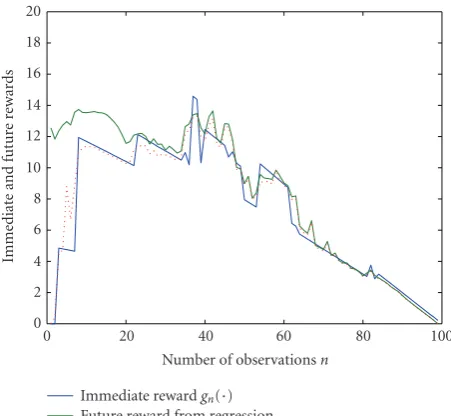
Immediate rewardgn(·) Future reward from regression Future reward from 1- step look- ahead Figure2: A sample path of reward values.
in the regression-based suboptimal policy,J =1000 sample paths were generated.
Figure 2depicts a sample path of the immediate reward gn(ψn) forn = 1, 2,. . .,N and a sample path of the future reward Vn(ψn) of the regression-based method as well as that of the one-step look-ahead policy, given by the r.h.s. of (40), for mean SNR = −3 dB andλ = 0. In this particular example, the one-step look-ahead policy declares “stop” at n=3 (the smallestnsuch that (40) is satisfied) with a reward of 4.8, while the regression-based policy stops at n = 26 (the smallestnsuch thatgn(ψn)>Vn(ψn)) to obtain a total rate reward of 11.7. If it were possible to make a noncausal decision after seeing allNobservations, a “genie-aided” rule would be able to maximize the objective in (25) over theUn’s that potentially depend onYN. Thus, the “genie-aided” rule asserts thatUn=stop for a givenλifnis the maximizer of
max n∈{1,2,...,N}gn
ψn;λ
. (46)
Since the feasible set of policies for the “genie-aided” case is a superset of that of the original problem (25), the optimal objective corresponding to the “genie-aided” rule represents an upper-bound to the throughput that can be obtained from the optimal sensing policy. In the particular example under discussion, the “genie-aided” rule would be able to achieve a reward of 14.6 by stopping at timen = 37, at which the maximum ofgn(ψn) is achieved.
0 0.005 0.01 0.015 0.02
C
o
llision
p
ro
babilities
0 100 200 300 400 500
Iterations (a)
0 10 20 30
Lag
range
m
ultipliers
0 100 200 300 400 500
Iterations (b)
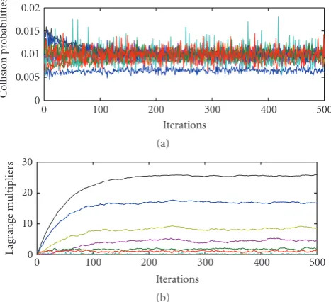
Figure 3: Evolution of the collision probabilities (a) and the Lagrange multipliers (b).
0 5 10 15 20 25 30
A
ver
age
thr
oug
h
put
−12 −9 −6 −3 0 3 6
Mean SNR (dB) Genie-aided
Regression-based
1-step look-ahead Optimized FSS Figure4: Average throughput versus mean SNR.
update algorithm is seen to converge and the collision probability constraints are met in each band.
Figure 4 plots the achieved average total rates of the proposed regression-based scheme when the mean SNR of the PU-to-CR channels is varied. For comparison, the average throughput of the genie-aided and the one-step look-ahead schemes are also shown. Averaging was performed over 2, 000 independent Monte Carlo realizations. It can be seen that the regression-based scheme attains throughput close to the genie-aided upper-bound over a wide range of SNR values. Also, the one-step look-ahead scheme is clearly suboptimal especially in the moderate-to-high SNR range.
0 10 20 30 40 50 60 70 80 90 100
P
er
centage
of
genie-aided
thr
o
ug
hput
ac
hie
ved
−12 −9 −6 −3 0 3 6
Mean SNR (dB) Regression-based
1-step look-ahead Optimized FSS
Figure5: The ratio of the average throughput achieved to the genie-aided throughput.
To compare the performance of the sequential regres-sion-based sensing policy to that of the batch scheme, the FSS test is designed and optimized in the following way. For the given set of channel gain values {G(m)} and
noise variance σ2, the detection threshold to satisfy the
misdetection probability constraint at the sample sizen is given by (8), and the corresponding false alarm probability by (7). Then, the average throughput due to the FSS test with sample sizencan be computed as
Efn(H,tn)
=T−nTs T
M
m=1
R(m)p(0m)
1−α(nm)
. (47)
The average throughput of the optimized FSS test is then defined as the value of
max
1≤n≤N,n∈NE
fn(H,tn)
, (48)
where the expectation is overH and{yn}. The sample size nfor the optimized FSS test is computed given the channel gains before receiving any samples. The computational complexity associated with the one-dimensional search in (48) is rather trivial.
Figure 4depicts the average throughput of the optimized FSS scheme versus the mean SNR level. It can be seen that the proposed regression-based sequential sensing scheme outperforms the optimized FSS over all SNR levels tested.
0 5 10 15 20 25 30
A
ver
age
thr
oug
h
put
−12 −9 −6 −3 0 3 6
Mean SNR (dB)
J=100
J=500
J=1000
J=1500
Figure6: The average throughput of the regression-based policy for different numbersJof simulated paths.
To test the sensitivity of the proposed algorithm to the number J of the simulated paths used for computing the regression coefficients an, Figure 6 plots the average throughput of the regression-based policy for different values ofJ. It can be seen that whenJ is as small as 100, there is some degradation in performance in the low SNR regime. However, the performance improvement as J is increased saturates very quickly whenJis larger than 500.
6. Conclusions
Sequential sensing algorithms for OFDM-based wideband CR systems have been developed. The tradeoffbetween the sensing time and the chance of identifying more unoccupied subchannels were captured in the effective rate achieved by the CR system. Optimal stopping problems were formulated, which maximized the effective rate given the past and current observations. Although a sufficient statistic with dimension lower than that of the accumulated samples was identified, the computational complexity of the optimal solution of the associated dynamic programming problem was still prohibitive. A basis expansion-based reduced-complexity solution was derived, whose performance was shown to be close to the genie-aided upper-bounds and hence close to that of the optimal solution.
In a companion paper [17], an extension to the cooper-ativesequential sensing will be considered. A recursive (on-line) version of the batch training procedure developed here will also be presented, which further reduces the computa-tional burden and the memory requirements associated with the batch counterpart developed here.
Acknowledgments
This work was supported by NSF Grants CCF 0830480 and CON 014658 and also through collaborative participation in
the Communications and Networks Consortium sponsored by the U.S. Army Research Laboratory under the Collabo-rative Technology Alliance Program, CoopeCollabo-rative Agreement DAAD19-01-2-0011. The U.S. Government is authorized to reproduce and distribute reprints for Government purposes notwithstanding any copyright notation thereon.
References
[1] Q. Zhao and A. Swami, “A survey of dynamic spectrum access: signal processing and networking perspectives,” in Proceedings of IEEE International Conference on Acoustics, Speech and Signal Processing (ICASSP ’07), vol. 4, pp. 1349– 1352, Honolulu, Hawaii, USA, April 2007.
[2] A. Sahai, N. Hoven, M. Mishra, and R. Tandra, “Fundamental tradeoffs in robust spectrum sensing for opportunistic fre-quency reuse,” Tech. Rep., University of California, Berkeley, Calif, USA, 2006.
[3] T. A. Weiss and F. K. Jondral, “Spectrum pooling: an innova-tive strategy for the enhancement of spectrum efficiency,”IEEE Communications Magazine, vol. 42, no. 3, pp. S8–S14, 2004. [4] S. Geirhofer, L. Tong, and B. M. Sadler, “Dynamic spectrum
access in the time domain: modeling and exploiting white space,”IEEE Communications Magazine, vol. 45, no. 5, pp. 66– 72, 2007.
[5] C. Cordeiro, K. Challapali, D. Birru, and N. Sai Shankar, “IEEE 802.22: the first worldwide wireless standard based on cognitive radios,” inProceedings of the 1st IEEE International Symposium on New Frontiers in Dynamic Spectrum Access Networks (DySPAN ’05), pp. 328–337, Baltimore, Md, USA, November 2005.
[6] D. Cabric, A. Tkachenko, and R. W. Brodersen, “Spectrum sensing measurements of pilot, energy, and collaborative detection,” in Proceedings of the Military Communications Conference (MILCOM ’06), pp. 1–7, Washington, DC, USA, October 2006.
[7] H. Urkowitz, “Energy detection of unknown deterministic signals,”Proceedings of the IEEE, vol. 55, no. 4, pp. 523–531, 1967.
[8] M. ¨Oner and F. Jondral, “On the extraction of the channel allocation information in spectrum pooling systems,” IEEE Journal on Selected Areas in Communications, vol. 25, no. 3, pp. 558–565, 2007.
[9] Z. Quan, S. Cui, A. H. Sayed, and H. V. Poor, “Optimal multiband joint detection for spectrum sensing in cognitive radio networks,”IEEE Transactions on Signal Processing, vol. 57, no. 3, pp. 1128–1140, 2009.
[10] Z. Quan, S. Cui, H. V. Poor, and A. H. Sayed, “Collaborative wideband sensing for cognitive radios,”IEEE Signal Processing Magazine, vol. 25, no. 6, pp. 60–73, 2008.
[11] J. Unnikrishnan and V. V. Veeravalli, “Cooperative sensing for primary detection in cognitive radio,”IEEE Journal on Selected Topics in Signal Processing, vol. 2, no. 1, pp. 18–27, 2008. [12] Y.-C. Liang, Y. Zeng, E. C. Y. Peh, and A. T. Hoang,
“Sensing-throughput tradeoff for cognitive radio networks,” IEEE Transactions on Wireless Communications, vol. 7, no. 4, pp. 1326–1337, 2008.
[13] D. Siegmund,Sequential Analysis, Springer, New York, NY, USA, 1985.
on Electronics, Circuits, and Systems, pp. 514–517, Marrakech, Morocco, December 2007.
[15] Y. S. Chow, H. Robbins, and D. Siegmund,Great Expectations: The Theory of Optimal Stopping, Houghton Mifflin Company, Boston, Mass, USA, 1971.
[16] J. Jia, Q. Zhang, and X. Shen, “HC-MAC: a hardware-constrained cognitive MAC for efficient spectrum manage-ment,”IEEE Journal on Selected Areas in Communications, vol. 26, no. 1, pp. 106–117, 2008.
[17] S.-J. Kim and G. B. Giannakis, “Sequential sensing for multi-channel cognitive radios,” submitted toIEEE Transactions on Signal Processing.
[18] S. M. Kay, Fundamentals of Statistical Signal Processing: Detection Theory, vol. 2, Prentice-Hall, Upper Saddle River, NJ, USA, 1993.
[19] Z. Quan, S. Cui, A. H. Sayed, and H. V. Poor, “Wideband spectrum sensing in cognitive radio networks,” inProceedings of the IEEE International Conference on Communications, pp. 901–906, Beijing, China, May 2008.
[20] D. P. Bertsekas,Dynamic Programming and Optimal Control, vol. 1, Athena Scientific, Belmont, Mass, USA, 2nd edition, 2000.
[21] T. S. Ferguson,Optimal Stopping and Applications, Mathemat-ics Department, UCLA, Los Angeles, Calif, USA.
[22] D. A. Casta˜non, “Approximate dynamic programming for sen-sor management,” inProceedings of the 36th IEEE Conference on Decision and Control (CDC ’97), vol. 2, pp. 1202–1207, San Diego, Calif, USA, December 1997.
[23] N. Z. Shor, Minimization Methods for Non-Differentiable Functions, Springer, New York, NY, USA, 1985.
[24] D. P. Bertsekas, “Convergence of discretization procedures in dynamic programming,”IEEE Transactions on Automatic Control, vol. 20, no. 3, pp. 415–419, 1975.
[25] J. N. Tsitsiklis and B. Van Roy, “Optimal stopping of Markov processes: hilbert space theory, approximation algorithms, and an application to pricing high-dimensional financial derivatives,”IEEE Transactions on Automatic Control, vol. 44, no. 10, pp. 1840–1851, 1999.
[26] J. N. Tsitsiklis and B. Van Roy, “Regression methods for pricing complex American-style options,”IEEE Transactions on Neural Networks, vol. 12, no. 4, pp. 694–703, 2001.