Single-neuron correlates of visual object
representation in the human brain: effects of
attention, memory, and choice
Thesis by Juri Minxha
In Partial Fulfillment of the Requirements for the degree of
Doctor of Philosophy
CALIFORNIA INSTITUTE OF TECHNOLOGY Pasadena, California
2018
I would be remiss if I did not mention my cohort of fellow CNS students. I specifically want to single out Gidi Nave and Luke Urban. Gidi was my first friend at Caltech, and his friendship over the years is something I truly cherish and hope to cultivate for the rest of my life. Luke and I had very similar trajectories through graduate school; we both started out working with brain-machine interfaces. Our light-hearted conversations over the years have often provided the much-needed break from the day-to-day grind.
I want to recognize all of my friends at Caltech, from whom I feel I have taken so much. Caltech is a small place and my friends are all from diverse fields. Sometimes it feels that my PhD was not just in neuroscience, but also astrophysics, computer vision, mathematics, etc.
I want to thank all the members of my Albanian family, Moza, Halit, Rudi, Edmond, Alba, Linda, and Kevin as well as my Brazilian family for their unwavering support throughout my time here.
temporal lobe are insensitive to such task conditions; and (3) spike-field coherence between field potentials in the medial temporal lobe and action potentials in the medial frontal cortex are enhanced during recognition memory choices. This suggests that inter-areal communication between these two brain regions may be facilitated selectively in tasks that rely on recognition memory-based information.
PUBLISHED CONTENT AND CONTRIBUTIONS
Minxha, Juri, et al. "Fixations gate species-specific responses to free viewing of faces in the human and macaque amygdala." Cell reports 18.4 (2017): 878-891.
Minxha, Juri, et al. “Surgical and Electrophysiological Techniques for Single-Neuron Recordings in Human Epilepsy Patients”In Extracellular Recording Approaches, Springer, Ed. Sillitoe, Roy, ISBN 978-1-4939-7548-8 (2018)
and effect of target ... 88
Figure 4.3: Separate neuronal populations in medial frontal cortex signal choice in a recognition memory and categorization task ... 92
Figure 4.4: MFC and not MTL neurons represent choice ... 93
Figure 4.5: Visually selective cells in the MTL are not sensitive to task demands ... 95
Figure 4.6: Visual information is stronger in MTL than it is in MFC ... 96
Figure 4.7: Category information in MFC is modulated by task ... 97
Figure 4.8: Choice cells are distinct from visually selective cells in The MFC ... 98
Figure 4.9: Phase-locking of hippocampal cells to local theta ... 99
Figure 4.10: MFC cell coherence with MTL theta is modulated by task ... 101
Figure 5.1: Labeling fixations and saccades from continuous eye-tracking data ... 112
Figure 5.2: Preferences for certain image categories and for novel images are apparent in the subject’s eye-movements ... 113
Figure 5.3: Fixation-aligned responses of cells in the human MTL encode the familiarity of the fixated item ... 114
Figure 5.4: Averaging fixation-aligned responses can lead to artifacts ... 115
Figure 5.5: Subsampling sequences of fixations to prevent artifacts from averaging ... 116
Figure 5.6: Covert attention task with distractors ... 117
Figure 5.7: Theta-frequency spike field coherence of an amygdala cell ... 119
Figure 6.1: MATLAB-based spike sorting tool ... 122
Figure 6.2: Bin-free time-since-last-spike (TSLS) latency estimation method .. 123
LIST OF TABLES
Number Page
Table 2.1: Example electrode locations ... 15
Table 2.2: Spike sorting algorithms commonly used for human single
NOMENCLATURE
ACC anterior cingulate cortexOver
AED anti-epileptic drug
BOLD blood-oxygen-level-dependent
CV coefficient of variation
DOS depth of selectivity
EEG electroencephalography
EPSP excitatory postsynaptic current
ERP event-related potential
FDR false discovery rate
fMRI functional magnetic resonance imaging
iEEG intracranial electroencephalography
ISI interspike interval
KS-test Komogorov-Smirnof goodness-of-fit test
LFP local field potential
mPFC medial prefrontal cortex
MUA multi-unit activity
OFC orbitofrontal cortex
PCA principal component analysis
PFC prefrontal cortex
pre-SMA pre supplementary motor area
RT reaction time
ROC receiver operator characteristic
SNR signal-to-noise ratio
SVM support vector machine
SUA single-unit activity
STD standard deviation
SEM standard error of the mean
TLE standard temporal lobe epilepsy
Rutishauser, U., et al. (2006). "Single-trial learning of novel stimuli by individual neurons of the human hippocampus-amygdala complex." Neuron 49(6): 805-813.
Rutishauser, U., et al. (2011). "Single-unit responses selective for whole faces in the human amygdala." Current Biology 21(19): 1654-1660.
Rutishauser, U., et al. (2013). "Single-neuron correlates of atypical face processing in autism." Neuron 80(4): 887-899.
Rutishauser, U., et al. (2015). "Representation of retrieval confidence by single neurons in the human medial temporal lobe." Nature neuroscience 18(7): 1041-1050.
Sheinberg, D. L. and N. K. Logothetis (2001). "Noticing familiar objects in real world scenes: the role of temporal cortical neurons in natural vision." Journal of Neuroscience 21(4): 1340-1350.
Siapas, A. G., et al. (2005). "Prefrontal phase locking to hippocampal theta oscillations." Neuron
46(1): 141-151.
Wang, S., et al. (2014). "Neurons in the human amygdala selective for perceived emotion." Proceedings of the National Academy of Sciences 111(30): E3110-E3119.
Chapter II: Surgical and Electrophysiological Techniques for Single-Neuron
Recordings in Human Epilepsy Patients
2.1 Overview
Extracellular recordings of single-neuron activity in awake behaving animals are one of the principal techniques used to decipher the neuronal basis of behavior. While only routinely possible in animals, rare clinical procedures make it possible to perform such recordings in awake human beings. Such human single-neuron recordings have started to reveal insights into the neural mechanisms of learning, memory, cognition, attention, and decision-making in humans. Here, we describe in detail the methods we developed to perform such recordings in patients undergoing invasive monitoring for localization of epileptic seizures. We describe three aspects: the neurosurgical procedure to implant depth electrodes with embedded microwires, electrophysiological methods to perform experiments in clinical settings, and data processing steps to isolate single neurons. Together, this chapter provides a comprehensive overview of the methods needed to perform single-neuron recordings in humans during psychophysical tasks.
2.2 Introduction
describe the method we have successfully employed for the last 12 years, but acknowledge that other methods or modifications may be equally successful.
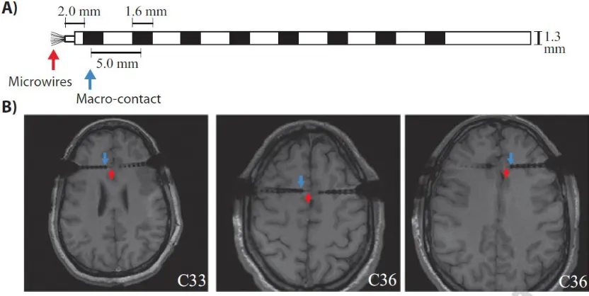
Figure 2.1: Electrodes used and postoperative MRIs. (a) Sketch of the hybrid macro-micro depth electrode. (b)
Example postoperative MRIs illustrating the depth electrode placement.
2.3 Surgical Methods
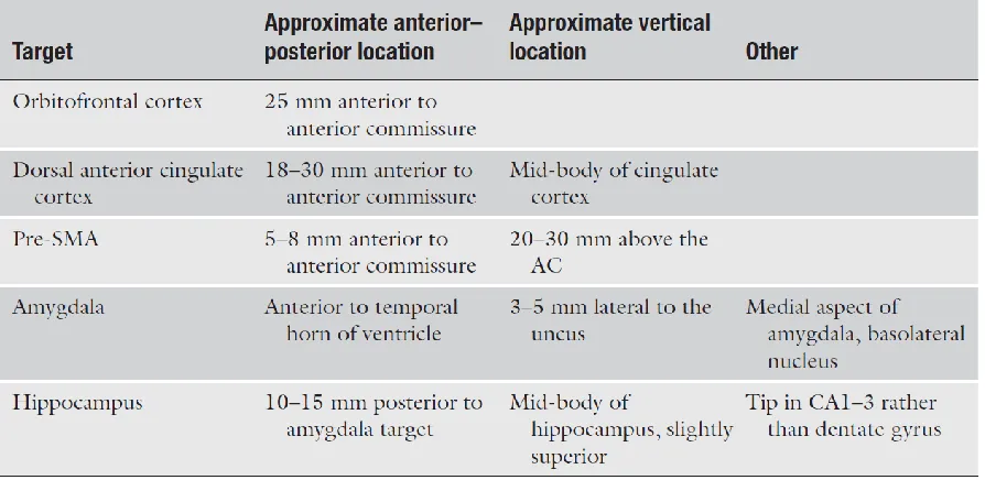
2.3.1 Target Selection
Failure to follow such strict ethical standards is likely to lead to potential harm to patients, which can never be justified.
In general, patients undergoing depth electrode monitoring fall into two categories: (1) seizures are suspected to arise from a medial temporal or limbic structure, but non-invasive monitoring and imaging tests are not sufficient to justify proceeding directly to a surgical intervention. Common examples of this include patients with suspected unilateral onset of seizures in the hippocampus or amygdala, but patients do not meet so called “skip” criteria, so that depth electrode monitoring is used to confirm that all the seizures arise from one mesial temporal lobe versus having bilateral independent seizure onsets, or evidence that the seizures do not arise from the mesial temporal lobe at all. Another common situation is a case where the patient is believed to have localization specific epilepsy, but non-invasive monitoring cannot reliably identify the site. In those cases, depth electrode monitoring is used both to determine lateralization (i.e. what hemisphere does a seizure focus arise from) and localization (i.e. from what lobe of the brain or general region does the seizure arise from). Often in these cases, patients subsequently go on to subdural grid or high density SEEG monitoring to further localize the seizures.
Table 2.1: Example electrode locations
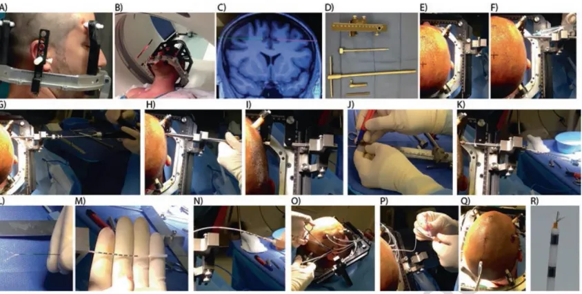
2.3.2 Stereotactic targeting
Depth electrodes need to be inserted with a high degree of precision. Both the final target position as well as the trajectory from the surface of the brain to the target must be
routinely utilized by the majority of neurosurgical centers around the world. With this method, a metal frame is attached to the patient’s head using 4 disposable screws that penetrate the skin and press on but do not go into the skull (Figure 1). We utilize ear bars inserted into the auditory canals of the patient at the time of frame placement to ensure a perfectly centered and orthogonal frame placement.
Together, this configuration allows us to connect only a single system to the patient, which lowers noise and avoids interference (see Notes 4 and 5). While we monitor the broadband recordings throughout the experiment, all processing of the data (i.e. filtering, spike detection, spike sorting) is redone during offline analysis. We typically set the input range to ±2500 µV, resulting in <1 µV resolution. This is especially critical for spike sorting (see below), which relies on the shape of the spike waveforms themselves. Alternative products from other manufacturers (including Blackrock Microsystems Inc. and TDT Inc.) offer similar solutions to the one we described.
2.4.2 Stimulus Presentation and eye tracking
We implement all experimental tasks in Matlab with Psychophysics Toolbox (Brainard 1997, Pelli 1997). This well-tested and extensively utilized toolbox has been utilized by numerous human intracranial experimenters and is well-suited for this purpose. We typically show stimuli on a 19-inch screen with a resolution of 1024 x 768 pixels. The screen is supported by an arm mount and also carries the camera and infrared light source for the eye-tracker. We monitor monocular gaze position with a 500Hz sampling rate with an Eyelink 1000 system (SR Research Inc.). We utilize a 9-point calibration grid to determine the
eye-to-screen coordinate transformation. Throughout a typical experiment, we can monitor eye
position with an accuracy of 0.42 DVA ± 0.15.
2.4.3 Response boxes and keyboards
2.4.6 Filtering
The first step in the processing pipeline is to remove low frequency content from the raw trace (Fig. 3a) by band-pass filtering the raw signal in the 300-3000 Hz frequency range (Fig. 3b). In order to preserve the shapes of the spike waveforms, it is important that the filtering process does not introduce phase distortions (Quiroga 2009), which is achieved by using a zero-phase digital filter ((Fig. 7). For real-time applications, such filtering is not possible because it is non-causal. In that case, the alternative is to use a linear phase FIR filter and directly account for the group delay introduced by the filter (delay = (L-1)/2, where L is the filter length).
Figure 2.3: Zero-phase filtering (a) Bandpass filtering is a common first step in improving the signal-to-noise ratio of spike waveforms. By retaining spectral information in a specific frequency range (300-3000 Hz for the example shown here), we can improve detection and sorting of spike waveforms. The way in which the filtering is performed however, can greatly change your results. Here we show the results when we filter the raw data (blue trace, Fs = 32000Hz) with no phase distortion (red trace) and when we filter in the conventional way (yellow trace). Zero-phase filtering was implemented with the Matlab function filtfilt. (b) While both methods preserve the waveform shape, conventional filtering delays the spike waveform while zero-phase filtering does not.
2.4.7 Spike detection and extraction
Ross et al. 2010, Kaminski, Sullivan et al. 2017) for examples). These include: projection tests between all possible pairs of clusters on the same wire (Pouzat, Mazor et al. 2002, Rutishauser, Schuman et al. 2006, Rutishauser, Ye et al. 2015), isolation distance (for each cluster versus all other detected spikes on a wire), L-ratio (Schmitzer-Torbert, Jackson et al. 2005, Hill, Mehta et al. 2011), %ISI violations <3ms, and signal-to-noise of the mean waveform of a cluster.
prominent waveform shapes, each one belonging to a different underlying unit (green and red), were identified on this channel. (E) The individual waveforms (256 samples per electrode) from the two clusters projected into principal component space. The clusters are well-separated. (F) Projection test to validate the separation between the two putative single-units (clusters). Shown are two overlapping histograms, each corresponding to one cluster. There was less than 1% overlap.
31. Tsao, D.Y., W.A. Freiwald, R.B. Tootell, and M.S. Livingstone, A cortical region consisting entirely of face-selective cells. Science, 2006. 311(5761): p. 670-674. 32. Rutishauser, U., O. Tudusciuc, S. Wang, Adam N. Mamelak, Ian B. Ross, and R.
Adolphs, Single-Neuron Correlates of Atypical Face Processing in Autism. Neuron, 2013. 80(4): p. 887-899.
33. Rutishauser, U., O. Tudusciuc, D. Neumann, A.N. Mamelak, A.C. Heller, I.B. Ross, L. Philpott, W.W. Sutherling, and R. Adolphs, Single-unit responses selective for whole faces in the human amygdala. Current Biology, 2011. 21(19): p. 1654-60.
34. Rutishauser, U., A.N. Mamelak, and R. Adolphs, The primate amygdala in social perception - insights from electrophysiological recordings and stimulation. Trends Neurosci, 2015. 38(5): p. 295-306.
35. Adolphs, R., F. Gosselin, T.W. Buchanan, D. Tranel, P. Schyns, and A.R. Damasio, A mechanism for impaired fear recognition after amygdala damage. Nature, 2005. 433(7021): p. 68-72.
36. Dal Monte, O., V.D. Costa, P.L. Noble, E.A. Murray, and B.B. Averbeck, Amygdala lesions in rhesus macaques decrease attention to threat. Nature communications, 2014. 6: p. 10161-10161.
37. Adolphs, R., D. Tranel, and A.R. Damasio, The human amygdala in social judgment. Nature, 1998. 393(6684): p. 470-474.
38. Mormann, F., S. Kornblith, R.Q. Quiroga, A. Kraskov, M. Cerf, I. Fried, and C. Koch, Latency and selectivity of single neurons indicate hierarchical processing in the human medial temporal lobe. Journal of Neuroscience, 2008. 28(36): p. 8865-8872.
39. Harris, K.D., D.A. Henze, J. Csicsvari, H. Hirase, and G. Buzsaki, Accuracy of tetrode spike separation as determined by simultaneous intracellular and extracellular
3.3.2 Electrophysiology
3.3.3 Fixation-target sensitive neuronal responses
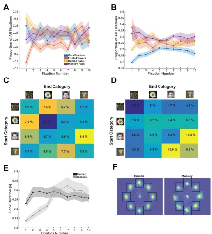
We further characterized the category selectivity of fixation-target sensitive responses (Fig. 2C,D). We first classified each fixation-target sensitive cell according to the category to which it responds most strongly (highest firing rate) at the point of time at which neurons provided most category information (see Methods and Fig. 3.6).
Figure 3.6: Using mutual information to determine the position of the analysis window for selectivity analysis, related to Figure 3. (A) Time-course of information, quantified as mutual information (MI; peak normalized) between the firing rate and visual category for all neurons recorded in monkeys (N=195, light gray) and humans (N=422, black). The point of time at which MI was maximal (t=325ms and 229ms, respectively) was used to place the analysis window for all further analysis.
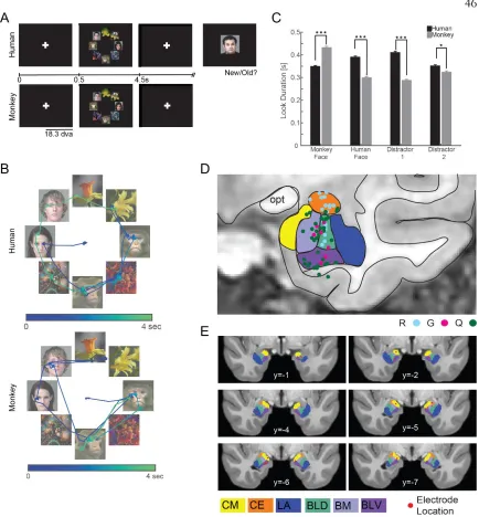
4C,D, see legends for statistics). Taken together, these observations show three important similarities between neurons in the human and monkey amygdalae: both contain fixation-target sensitive neurons; these neurons show category-specific responses; and the largest subset of such neurons responds preferentially to conspecific faces. A difference between the species was that human neurons have a sparser response profile over categories.
Figure 3.8: Monkey and human amygdala cells differ in their depth-of-selectivity. (A) Single-cell ROC analysis example. The monkey cell shown (identical to that in Fig. 2D) responded only to images of conspecifics, allowing it to discriminate 3 pairs of categories (dashed colored lines). (B) Distribution of the number of significant contrasts (see A) for all visually tuned neurons in humans (black) and monkeys (gray). Cells recorded in monkeys differentiated significantly more contrasts (4.15±0.2) than human cells (3.47±0.1, p<0.002, 2-sample KS test). (C,D) Population summary. Comparison of depth-of-selectivity (DOS) values for tuned and untuned cells in human (C) and monkey (D). In both species, the DOS values are significantly greater in the tuned population (p<1e-16, in humans and p<5e-5 in monkeys, 2-sample KS test). For tuned cells, DOS values were calculated for a subset of fixations that were not used in the selection of that cell (i.e. to determine its tuning). (E) Depth-of-selectivity (DOS) for all visually tuned neurons in humans (black) and monkeys (gray). Human cells had significantly larger DOS values (0.51±0.02 vs. 0.43±0.03, p<0.0003, 2-sample KS-test).
3.3.4 Interspecies comparison of response latencies of face-selective neurons
Figure 3.10: Face cells responded earlier and more strongly to conspecific compared to heterospecific faces. (A)Proportion of all recorded cells in humans (out of N=422) selective for fixations on conspecific (Hh, yellow) and heterospecific faces (Hm, purple). Shading indicates the 99% confidence interval. (B)Proportion of all recorded cells in monkeys (out of N=195) selective for fixations on conspecific (Mm, purple) and heterospecific (Mh, yellow) faces. (C,D)Average AUC as a function of time. Dotted colored lines indicate the 99% confidence interval.
3.3.5 Category-preference of fixation-sensitive neurons during covert attention
Using look-onset instead of fixations
Figure 3.12: Comparison of fixation onset and look onset methods, related to Figure 1. (A) Example scan path from a single trial from a human subject. See Fig 3.1 for notation. (B) Summary of eye-tracking data into discrete periods of "looks" (yellow squares). Successive fixations that fall on the same image are pooled together into a single "look". The y-axis denotes the location of the look in the array as indicated in (A). (C, D) Comparison of a single-cell response, aligned to fixation onset (C) and look onset (D). Note the virtually identical response of the cell using the two criteria. For each, Raster and PSTH are shown. (E) Cumulative distribution for fixation (red) and look (blue) duration. Look duration was longer because of the pooling of several fixations into one look. (F) Same as (E), but for monkeys.
Selection of units
Spitler, K.M., and Gothard, K.M. (2008). A removable silicone elastomer seal reduces granulation tissue growth and maintains the sterility of recording chambers for primate neurophysiology. J Neurosci Methods 169, 23-26.
Tyszka, M.J., and Pauli, W.M. (2016). A high resolution in vivo MRI atlas of the adult human amygdaloid complex. submitted.
differences in reaction time within condition, between the two different responses (i.e. “yes” and “no”). In the memory condition, subjects were significantly slower at saying “no” than “yes” (Figure 4.2 A). This is a common pattern in recognition memory tasks, and thus shows that subjects utilize recognition memory (Stern and Hasselmo 2009) . In contrast, in the visual categorization condition, subjects were slower at saying “yes” than “no” (Figure 4.2 B). These condition differences were evident at the level of individual sessions (Figure
4.2C, p = 1.4e-7 for memory condition, p = 0.03 for category condition, t-test). Making a
Figure 4.1: Task, behavior, and electrode locations (a) The subjects responded using either their hands (example trial on top) or by saccading to one of the target locations on the left and right of the image (example trial on the bottom). Yes and No responses are always on the left and right respectively. The subject is told how to respond (i.e. hand versus saccade) and to what question (i.e. recognition memory versus image categorization) to address at the beginning of each block (40 images/block). The question varied block by block, with category and recognition memory questions interleaved over the 8 blocks. The first block was always an image categorization block. For each of the categorization blocks, the target category was randomly assigned to one of the four available image categories. (b) Locations of the MTL electrodes, with hippocampal electrodes shown in yellow and amygdala electrodes shown in magenta. (c) MFC electrodes with pre-SMA electrodes shown in red and dACC electrodes shown in blue. (d) Eye-tracking data from an example session, showing only the trials with button press (160/320 trials). (e) Same as (c) but for eye response (160/320 trials). Note that the subject only breaks fixation on the center of the image in order to make the response. (e) Reaction time differences between the two conditions (memory condition, mean± sem, 1.22 ±0.017s; category condition, 0.89 ± 0.02s; p = 2.5e-216, 2-sample KS test). (g) Performance on memory questions improves over the course of the experiment (p<1e-10, logistic regression, mixed effects model). (h) Memory performance by image category.
Figure 4.2: Yes vs. No differences in memory and categorization trials and effect of target
(a) Cumulative distribution of reaction times for “yes” and “no” responses during the memory trials shown for all included sessions. Subjects were significantly slower at saying “No, I have not seen that image before” than “Yes, I have seen that image before.” (b) Same as (a) but for the categorization trials. (c) Plotted for each session, is the mean difference between “yes” and “no” responses shown separately for memory trials (green, p=1.2773e-16, t-test) and categorization trials (yellow, p = 6.2e-6, t-test). (d) Making a category the target on a categorization block does not enhance memory for that category on follow-up memory blocks. (e)
separately only for memory trials in MFC and MTL (Figure 4.4 D, left panel included all trials, right panel is only for memory choice trials). In both tests, choice information was significantly stronger in the MFC population than in MTL (p = 1.87e-24 for all trials; p = 4.58e-21 mem trials; paired t-test, measured at t = 750ms after stimulus onset). This shows a clear functional separation between these two areas, with MTL cells representing features that pertain to the stimulus itself and MFC cells representing choice.
Figure 4.3: Separate neuronal populations in medial frontal cortex signal choice in a recognition memory and categorization task. (a) Example choice cells in MFC. This example ACC cell fires preferentially for “yes” (i.e. “I have
seen this before”) responses in the memory condition. Raster condition PSTH (i.e. memory versus visual categorization), and choice PSTH (each condition is split into “yes” versus “no” traces) correspond to the top, middle, and bottom panels respectively. (b) An example cell recorded from pre-SMA that preferentially fires for “no” (i.e. “I have not seen this image before”) responses in the memory condition. (c) Average PSTH for cells that separate “yes” versus “no” in the visual categorization condition only (top panel). Also shown, is the average PSTH for the “yes” and “no” responses
information on categorization trials (blue condition, p=0.32, permutation test of the mean). Memory choice cells represent choice and not a recognition memory signal during the recognition trials (green vs. red trace, p<0.005, paired t-test). On the right, yellow bar = “yes” versus “no” information in category choice cells (n=32) as measured by AUC (mean ± sem) on categorization trials, blue bar = “preferred category” versus “non-preferred category” on recognition memory trials, where preferred is defined by the target in the preceding categorization block. Category choice cells do not contain category information (blue condition, p=0.41 permutation test).
cells (Figure 4.5H). At the population level, representation of image category is much stronger in MTL than in MFC, both when we use all available trials (Figure 4.6B, p = 3.1e-66, paired t-test, evaluated at peak decoding accuracy for each area independently) and when we only use memory trials (Figure 4.6C, p = 6.7410e-38, paired t-test, evaluated at peak decoding accuracy). Together, this result shows that representations in the MTL population are stable and not sensitive to task demands. Furthermore, this data again highlight the difference between the stable, stimulus-specific representations in the MTL, and the representations of task-specific variables that we find in MFC cells.
Figure 4.5: Visually selective cells in MTL are not sensitive to task demands
Decoding results across each of the subpopulations that are tuned to the different image categories. Average decoding performance is above chance (99 % CI of the null distribution shown with the black dotted line) and qualitatively comparable across all categories. (e) Number of significant pairwise AUC comparisons (4 categories = 6 possible pairwise comparisons). (f) Average effect size for all visually selective cells, split by condition, shows no preference for task type. (g) Comparison of AUC values for category and memory trials shows no difference (p = 0.38, t-test). (h) Using the same selection criteria as that outlined for the choice cells, we find n = 17/360 cells (p=0.53) tuned for memory choice, and n = 23/360 (p=0.1) cells for category choice, much weaker than MFC cells.
Figure 4.6: Visual information is stronger in MTL than it is in MFC
4.3.5 Category information in the MFC cells is modulated by task demands
We next tested to see if category information was also present in MFC cells. Selection for visually selective MFC cells was done using a 1s window centered at 700 after stimulus onset [200 – 1200ms]. Note that this is the same window that was used for the choice-selective cells in MFC. We isolated 62/399 visually selective cells using a 1x4 ANOVA with a threshold of p<0.05. Unlike the MTL cells, category tuning in the MFC was strongly modulated by task condition (see Figure 4.7 A, B for examples). When we computed Ω2- effectize (Figure 4.7 C) for image category in the memory and categorization conditions separately, we found that it was signitifantly higher in the memory condition, both at the population level (p = 1.5e-6, paired t-test) and for the selected cells (p = 1.7e-4, paired t-test). When selecting for visually tuned cells indepednetly in the memory and categorization condition, we found a significantly larger proportion of cells in the memory condition (Figure 4.7 D, 60 vs. 29 cells; χ2 – 12.15, p = 4.9e-4). This difference was also apparent at the population level, as revealed by the decoding results (Figure 4.7 E). For the decoding, we used the entire population of cells, not just the visually selective ones. The decoding method is the same as that outlined in the previous sections (see Methods).
Figure 4.7: Category information in the MFC cells is modulated by task
(a) Example raster of a cell in the medial-frontal cortex. The raster plots are split by image category. The left panel shows all the trials from the visual categorization condition and the right panel shows all trials from the memory condition. (b)
(cyan). Cell selection was done using all trials. Effect size was then measured independently on memory trials and categorization trials. The effect size is greater during the memory condition. d) Selecting independently, using only categorization trials or memory trials yields a much larger number of cells in the memory condition versus the categorization condition. (e) Decoding accuracy across the entire pseudo-population of MFC cells is much higher during the memory condition than the categorization condition.
4.3.6 Choice cells are distinct from visually selective cells in the MFC
We have identified choice-selective and visually-selective cells in the medial frontal cortex. The next step is to determine if these two pieces of information are carried by the same set of cells or if they are distinct populations. To do so, we computed the Ω2- effect size for choice (4 possible responses, yes/no ⊗ categorization\memory) as well as the Ω2- effect size for image category (4 image categories). Figure 4.8A shows the effect sizes for choice (x-axis) and image category (y-axis) across the entire population (in pink), choice cells (in green), and image category cells (in blue). The populations were largely disjointed, with only 15 cells showing tuning for both image category and choice.
Figure 4.8: Choice cells are distinct from visually selective cells in the MFC. (a) Ω2-effect size for image category and choice computed across all trial. (b) Proportion of cells selected as choice and as visually selective (here termed category cells) cells in the MFC.
4.3.7 Phase locking of hippocampal cells to local theta
.
[47%] of hippocampal cells had a significant preference to theta-frequency LFP; See Figure 4.9A-E). This data is important for two reasons: (1) it shows that hippocampal theta is prominent in our
task and that we are able to record it, and (2) it allows us to observe whether cells recorded in the MFC functionally interacted with the hippocampus and whether this interaction was modulated by task demands. Task modulation is not observed locally in the hippocampus, as shown in Figure 4.9G-F. Figure 4.9F shows that there is no difference in the spike triggered power of the theta
oscillations while Figure 4.9G demonstrates that there is no difference in how well hippocampal cells cohere to theta as a function of task.
Figure 4.10: MFC cell coherence with MTL theta is modulated by task
(a) Outline of the inter-area spike-field coherence measurement between spikes recorded in MFC and local-field potential recorded in the hippocampus. (b) Top: Example aligned trace and spikes. Shown in light gray is the raw, unfiltered trace (apart from antialiasing filter prior to down sampling to 250 Hz) and the 3-8 Hz filtered blue trace. Superimposed on top of the raw and filtered trace, are the spike locations. Bottom: A polar histogram of the extracted phase from the filtered trace (blue) for every spike recorded from this cell. The mean resultant vector is shown in red. The p-value from the Rayleigh test for this cell is p = 1e-12, shown very strong phase preference. (c) Selecting MFC cells as a function of delay in both inter-area coherence with hippocampal LFP (left) and within area coherence (right). (d) Number of tuned cells as a function of delay time, shown for all spikes (gray area), memory condition (blue area), and categorization condition (red area). The trace at the bottom shows the p-value from a t-test comparing Rayleigh’s z-value for selected cells, during the two task conditions.
4.4 Discussion
Shadlen, M. N. and D. Shohamy (2016). "Decision making and sequential sampling from memory." Neuron 90(5): 927-939.
Siapas, A. G., et al. (2005). "Prefrontal phase locking to hippocampal theta oscillations." Neuron 46(1): 141-151.
Sigurdsson, T., et al. (2010). "Impaired hippocampal–prefrontal synchrony in a genetic mouse model of schizophrenia." Nature 464(7289): 763-767.
Squire, L. R. (1992). "Memory and the hippocampus: a synthesis from findings with rats, monkeys, and humans." Psychological review 99(2): 195.
Stern, C. E. and M. E. Hasselmo (2009). Recognition Memory A2 - Squire, Larry R. Encyclopedia of Neuroscience. Oxford, Academic Press: 49-54.
The capacity to accurately recognize an item as having been previously encountered is known as recognition memory. In this article, the concept of recognition memory is discussed, including the idea that recognition memory is composed of two main components: recollection and familiarity.
Neuroscience research examining recognition memory in humans and in animal models is described, besides the computational models of recognition.
Swanson, L. (1981). "A direct projection from Ammon's horn to prefrontal cortex in the rat." Brain research 217(1): 150-154.
Tyszka, J. M. and W. M. Pauli (2016). "In vivo delineation of subdivisions of the human amygdaloid complex in a high‐resolution group template." Human brain mapping 37(11): 3979-3998.
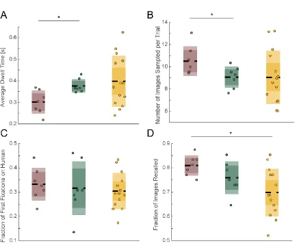
not shown here, we can also quantify a subject’s look preferences by their sampling sequence (see Figure 3.3), number of within-stimulus fixations, and look-time for each category (see Figure 3.1). Subjects also have preferences for novelty (Figure 5.2 B, C, D). When measured across the population, number of visitations is significantly correlated with the amount of time spent looking at the image (mixed-effects model across subjects, with random-effects on the intercept, p<2e-21). Furthermore, this effect can be seen on the individual categories, cars, humans, and fruits, but not on monkeys, which, across all subjects, are the hardest image category to remember (Figure, 5.2E, as measured on the recognition portion the subjects performed at the end of the array task). Looking time is often used in animal experiments as a proxy for whether something is perceived as familiar or novel (visual preference looking task, (Murray and Mishkin 1998, Zola, Squire et al. 2000).
Figure 5.2: Preferences for certain image categories and for novel images are apparent in the subject’s eye movements. (A) Proportion of first fixations on each of the four categories, computed over all recorded sessions. The preferred category is human faces, which is significantly more likely to be a target than the next best category, which is monkey faces (p <8e-04, paired t-test). (B) Look duration as a function of the number of fixations that landed on a particular image (bars are s.e.m). (C) Same as (B) but shown separately for three of the categories. (D) Same as (C) and (B) but for monkey fixations. For (B), (C), (D), the look durations were first standardized within the subject prior to averaging across the whole population. (E) Proportion of category instances remembered in the recognition memory task that followed the free-viewing task.
Figure 5.3: Fixation-aligned responses of cells in the human MTL encode the familiarity of the fixated item. (A,B) Example cells recorded in the human hippocampus (left) and amygdala (right) during the array task described in Chapter III. (C) A cell that is preferentially modulated by a novel face (recorded in amygdala).
5.3 Relating neural patterns with eye-movement data
process that was used for determining visually-selective cells in the array task. The selection criteria ranges from the most lax, which corresponds to a simple threshold on duration of fixation (or “look”), all the way to more strict criteria that only use the very first fixation on an image category.
Figure 5.5: Subsampling sequences of fixations to prevent artifacts from averaging. (A) Example scan-path recorded from a monkey. Numbers indicate “location on array”. (B) For trial shown in (A), summary of where the monkey looked. All successive fixations that fall on the same image are pooled into one "look" (Yellow patch). The looks are numbered 1-10 and the y-axis indicates the location on the array. (C) Different selection criteria for “looks” that can be included in the analysis. In the most lenient case, we can use all fixations that are longer than 100ms, and in the most stringent case, we can use only the first fixation for each category in addition to the duration requirement.
5.4 Covert spatial attention task with distractors
preferential tuning for one of the image categories (selected with 1x4 ANOVA and assigned to the image category that elicited highest firing rate). Figure 5.6 B shows the responses from two example cells split across the four possible conditions. The conditions are: (1) both the cued and the distractor were preferred (blue); (2) only the cued image was from the preferred category (red); (3) only the distractor was from the preferred category; and (4) neither the preferred image nor the distractor were from the preferred category.
Figure 5.6: Covert attention task with distractors. (a) Task design for the covert attention task. Subjects were cued to the spatial location of the stimulus for which they had to answer a question (e.g. “Is this a human face?”). After a short delay, two objects were presented on opposite ends of the array. Subjects responded with a button press, while always maintaining fixation. (b) Raster for two example cells showing the response in the four task conditions. (c) Population average across 22/120 amygdala cells that showed preferential tuning for one of the four possible image categories.
5.5 On the role of face responses in the amygdala
References
Chang, L. and D. Y. Tsao (2017). "The Code for Facial Identity in the Primate Brain." Cell
169(6): 1013-1028. e1014.
Murray, E. A. and M. Mishkin (1998). "Object recognition and location memory in monkeys with excitotoxic lesions of the amygdala and hippocampus." Journal of Neuroscience 18(16): 6568-6582.
Pessoa, L. and R. Adolphs (2010). "Emotion processing and the amygdala: from a'low
road'to'many roads' of evaluating biological significance." Nature reviews neuroscience 11(11): 773-783.
Phelps, E. A. (2004). "Human emotion and memory: interactions of the amygdala and hippocampal complex." Current opinion in neurobiology 14(2): 198-202.
Wang, S., et al. (2017). "The human amygdala parametrically encodes the intensity of specific facial emotions and their categorical ambiguity." Nature Communications 8.
Appendix
There is a variety of methods and tools that were developed and either not used or used too sporadically to be mentioned in the main text of this thesis. I am including them here because I believe that they still represent a unique way of looking at behavioral and neural data and could potentially be useful for future applications.
7.1 A MATLAB interface for processing spikes
7.2 A bin-free method for measuring onset latency