Applying Random Indexing to Structured Data
to Find Contextually Similar Words
Danica Damljanovi´c
∗, Udo Kruschwitz
†, M-Dyaa Albakour
†, Johann Petrak
∗2, Mihai Lupu
†2∗Department of Computer Science, University of Sheffield, United Kingdom, [email protected]
†School of Computer Science and Electronic Engineering, University of Essex, United Kingdom, udo,[email protected]
∗2Austrian Research Institute for Artificial Intelligence, Vienna, Austria, [email protected]
†2Vienna University of Technology, Vienna, Austria, [email protected]
Abstract
Language resources extracted from structured data (e.g. Linked Open Data) have already been used in various scenarios to improve conventional Natural Language Processing techniques. The meanings of words and the relations between them are made more explicit in RDF graphs, in comparison to human-readable text, and hence have a great potential to improve legacy applications. In this paper, we describe an approach that can be used to extend or clarify the semantic meaning of a word by constructing a list of contextually related terms. Our approach is based on exploiting the structure inherent in an RDF graph and then applying the methods from statistical semantics, and in particular, Random Indexing, in order to discover contextually related terms. We evaluate our approach in the domain of life science using the dataset generated with the help of domain experts from a large pharmaceutical company (AstraZeneca). They were involved in two phases: firstly, to generate a set of keywords of interest to them, and secondly to judge the set of generated contextually similar words for each keyword of interest. We compare our proposed approach, exploiting the semantic graph, with the same method applied on the human readable text extracted from the graph.
Keywords:rdf, ontologies, synonyms, contextually related words, random indexing
1.
Introduction
Language resources extracted from structured data (e.g. Linked Open Data cloud1) have already been used in various scenarios to improve conventional Natural Lan-guage Processing (NLP) techniques. For example, in the Question-answering system PowerAqua (Lopez et al., 2006), theOWL:SAMEASrelation is used to find synonyms in addition to those found using conventional methods such as through WordNet (Fellbaum, 1998). The meanings of words and the relations between them are made more ex-plicit in semantically structured knowledge sources such as RDF graphs, in comparison to human-readable text, and hence have a great potential to improve legacy applications. Statistical semantics methods such as Latent Semantic Analysis (LSA) and Random Indexing (RI) can be applied to derive the indirect relations between words. Latent Se-mantic Analysis (LSA) (Deerwester et al., 1990) is one of the pioneer methods which has been used for finding words based on contextual similarity (e.g. synonyms). The as-sumption behind this and other statistical semantics meth-ods is that words which appear in the similar context (with the same set of other words) are synonyms. Synonyms tend not to co-occur with one another directly, so indirect infer-ence is required to draw associations between words which are used to express the same idea (Cohen et al., 2009). The method has been shown to approximate human perfor-mance in many cognitive tasks such as the Test of English
1http://linkeddata.org
as a Foreign Language (TOEFL) synonym test, the grading of content-based essays and the categorisation of groups of concepts (see (Cohen et al., 2009)). RI can be seen as an approximation to LSA which is shown to be able to reach similar results (see (Karlgren and Sahlgren, 2001) and (Co-hen and Hunter, 2008)).
LLD1 LLD2 number of representative subgraphs 5000 50000
number of statements 595798 4573668
number of virtual documents 64644 473742
number of terms 417753 1713349
Table 1: Sizes of LLD1 and LLD2 datasets
Dataset Mean Std. Deviation
Group 1 LLD1 0.54 0.28
LLD2 0.46 0.31
Pubmed abstracts 0.33 0.28
Table 3: The dispersion values for the distribution of MAP across three datasets for the training model
5.
Results
In this section we first look into the results of training the model and finding the best parameters. Then, we look at the results of testing the RI method using these parameters.
5.1. Training the model
We expect to see variations of MAP, for different values of dimensionality, seed length, and minimum term frequency parameters. Our goal is to find the combination of parame-ters for which MAP is highest, so as to use those in future applications of the method.
As we can see in Table 3, results were better with LLD1 in comparison to LLD2, and this difference is statistically sig-nificant (p <0.0001, Independent-samples Mann-Whitney U Test). The reason is the high frequency of 0 values for the LLD2 dataset. However, results with LLD2 are still better in comparison to those with the baseline.
Looking closely into the differences of Average Precision per keyword for LLD1 and LLD2 datasets, the value for MAP seems to be constantly better for LLD1 in comparison to LLD2, with the termPTSDbeing the only exception (see Figure 2).
Figure 2: Correlation of Average Precision (AP) for LLD1 (X axis) and LLD2 (Y axis) per keyword
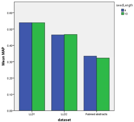
The seed length parameter did not have any significant influence (p=0.714 for LLD1 and p=0.914 for LLD2,
Independent-samples Mann-Whitney U Test), see Figure 3. We see this as a positive result, given that the computational resources (RAM in particular) are proportional to the value of seed length.
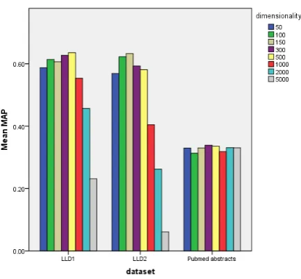
However, the wider span of dimensionality parameter made a significant difference to the value of MAP for LLD1 and LLD2 datasets, see Figure 4 (p < 0.0001, Independent-samples Kruskal-Wallis test). The peak for LLD1 was the dimensionality 500, while surprisingly the peak for the larger dataset was quite low, with the dimensionality set to 150. The variation of dimensionality parameter did not have a significant difference on MAP for the baseline model.
Similarly, the variation ofminimum term frequencycaused the fluctuation of the results, see Figure 5, with peaks for both LLD1 and LLD2 datasets at the maximum value of this parameter which was 25. For the baseline model, the peak was much lower (5). The difference in MAP caused by the variation ofminimum term frequencyfor all datasets is statistically significant (p < 0.0001, Independent-samples Kruskal-Wallis test).
Figure 3: The effect of the variation of seed length onMAP, forGroup 1used as the training set
Table 4 summarizes the best parameters: those that we chose to use in the testing phase.
5.2. Testing the model
Using the best parameters selected in the training phase, we now test whether the same setting can be used for a different, future set of terms.
Figure 4: The effect of the variation of dimensionality on MAP, for the Group 1 used as the training dataset
Figure 5: The effect of the variation of minimal term fre-quency onMAP, for the Group 1 used as the training dataset
shown in Table 5. The RI method results in a smaller value of MAP in the testing phase in comparison to the best trained model for all datasets.
Figure 6 shows the values of average precision per key-word, divided by dataset. The results vary across different keywords and all datasets seem to have peaks for some of the keywords. However, only the baseline resulted in
pro-Group 1
Dataset LLD1 LLD2 Pubmed abstracts
Min frequency 25 25 5
Seed length 4 4 4
Dimensionality 500 150 300
MAP 0.60 0.60 0.47
Table 4: Optimal parameters chosen forGroup 1 used as training sets
Group 2
Dataset LLD1 LLD2 Pubmed abstracts
Min frequency 25 25 5
Seed length 4 4 4
Dimensionality 500 150 300
MAP 0.425 0.48 0.26
Table 5: Testing the Random Indexing method usingGroup 2as thetestingset
ducing 0 for as much as 25% of the observed keywords, unlike the two other datasets which always yielded posi-tive average precision. The baseline yielded best results for 2 out of 12 keywords (16.67%), while LLD1 yielded bet-ter results for 4/12 keywords (33.33% of the cases). LLD2 produced best results in majority of the cases, namely for 6 out of 12 keywords (50% of the cases).
Figure 6: Mean Average Precision per keyword, by each dataset
Human assessment. In our previous work (Damljanovi´c et al., 2011b), we reported the Inter-annotator agreement usingObserved agreementandCohen’s Kappa agreement. The observed agreement across all keywords was 0.81, and the Cohen’s Kappa was 0.61 which indicates that the given task of selecting relevant keywords for a topic of interest was indeed difficult for domain experts. Relative to this dif-ficulty, we can conclude that our proposed method reaching the average MAP of 0.45 across LLD1 and LLD2 datasets is a very promising starting point to explore this approach further. Although this can be further improved, it is still much higher in comparison to the baseline model which applies the same method on the text of the abstracts instead of exploring the RDF structure.
6.
Conclusion
con-chies from text. InProceedings of the 22nd Annual Inter-national ACM SIGIR Conference on Research and De-velopment in Information Retrieval (SIGIR 1999), pages 206–213. ACM.
L. Sitbon and P. Bruza. 2008. On the relevance of docu-ments for semantic representation. InProceedings of the 13th Australasian Document Computing Symphosium, Hobard, Australia, December.
R. Snow, D. Jurafsky, and A. Ng. 2005. Learning syntactic patterns for automatic hypernym discovery. Advances in Neural Information Processing Systems, 17:1297–1304. M. Thelen and E. Riloff. 2002. A bootstrapping method for learning semantic lexicons using extraction pattern con-texts. InProceedings of the 2002 Conference on Empir-ical Methods in Natural Language Processing (EMNLP 2002), volume 10, pages 214–221. ACL.
G. Tummarello, R. Delbru, and E. Oren. 2007. Sindice.com: Weaving the Open Linked Data. In Pro-ceedings of the 6th International Semantic Web Confer-ence, Busan, Korea.