University of Windsor University of Windsor
Scholarship at UWindsor
Scholarship at UWindsor
Electronic Theses and Dissertations Theses, Dissertations, and Major Papers
2012
Query selection in Deep Web Crawling
Query selection in Deep Web Crawling
YAN WANG
University of Windsor
Follow this and additional works at: https://scholar.uwindsor.ca/etd
Recommended Citation Recommended Citation
WANG, YAN, "Query selection in Deep Web Crawling" (2012). Electronic Theses and Dissertations. 418.
https://scholar.uwindsor.ca/etd/418
Query Selection in Deep Web Crawling
by
Yan Wang
A Dissertation
Submitted to the Faculty of Graduate Studies
through Computer Science
in Partial Fulfillment of the Requirements for
the Degree of Doctor of Philosophy at the
University of Windsor
Windsor, Ontario, Canada
2012
c
Query Selection in Deep Web Crawling
by
Yan Wang
APPROVED BY:
Dr. Chengzhong Xu, External Examiner
Wayne State University
Dr. Xiang Chen
Department of Electronic Engineering
Dr. Arunita Jaekel
Department of Computer Science
Dr. Dan Wu
Department of Computer Science
Dr. Jessica Chen, Co-supervisor
Department of Computer Science
Dr. Jianguo Lu, Co-supervisor
Department of Computer Science
Dr. Chunhong Chen, Chair of Defense
Department of Electronic Engineering
Declaration of Previous
Publication
This thesis includes three original papers that have been previously published in blind reviewed journal and conference proceedings, as follows:
Thesis Chapter Publication title/full citation Publication status Part of Chapter
3
Yan Wang, Jianguo Lu and Jessica Chen. Crawling Deep Web Using a New Set Cover-ing Algorithm. ProceedCover-ings of 5th International Conference On Advanced Data Mining and Ap-plications (ADMA’09), page 326-337, Springer.
published
Major part of Chapter 4
Yan Wang, Jianguo Lu, Jie Liang, Jessica Chen, Jiming Liu. Selecting Queries from Sample to Crawl Deep Web Data Sources , Web Intelli-gence and Agent Systems, 2012.
published
Jianguo Lu, Yan Wang, Jie Liang, Jiming Liu and Jessica Chen. An Approach to Deep Web Crawling by Sampling, Proceedings of the 2008 IEEE/WIC/ACM International Conference On Web Intelligence (WI’08). Page:718-724.
published
Abstract
In many web sites, users need to type in keywords in a search Form in order to access the pages. These pages, called the deep web, are often of high value but usually not crawled by conventional search engines. This calls for deep web crawlers to retrieve the data so that they can be used, indexed, and searched upon in an integrated environment. Unlike the surface web crawling where pages are collected by following the hyperlinks embedded inside the pages, there are no hyperlinks in the deep web pages. Therefore, the main challenge of a deep web crawler is the selection of promising queries to be issued.
This dissertation addresses the query selection problem in three parts: 1)Query selection in an omniscient setting where the global data of the deep web are avail-able. In this case, query selection is mapped to the set-covering problem. A weighted greedy algorithm is presented to target the log-normally distributed data. 2)Sampling-based query selection when global data are not available. This thesis em-pirically shows that from a small sample of the documents we can learn the queries that can cover most of the documents with low cost. 3) Query selection for ranked deep web data sources. Most data sources rank the matched documents and return only the top k documents. This thesis shows that we need to use queries whose size is commensurate with k, and experiments with several query size estimation methods.
Dedication
To our heroes
Acknowledgements
I would like to acknowledge the important role of my PhD committee and the External Examiner, and thank them for their enlightening and encouraging com-ments and reviews.
I wish to express my gratitude to Dr.Jianguo Lu and Dr.Jessica Chen, my co-supervisors, for their valuable assistance and support during my thesis work, and for their persistent guidance through out my study during Ph.D. program. Especially for Dr. Chen, she has guided me for seven years since I was 24 years old. She gives me spirit and soul.
To my parents, I owe your everything and I can never fully pay you back what-ever I say or do. I love you and I miss you even when you are next to me. To my elder brother and younger sister, I appreciate you for many years support and own you for taking my duty to parents without any complaint.
To my fiancee, Nan Li, many years lonely waiting takes away your passion, your beauty and your youth. But the one thing never changed is your will to helping me fulfil my dream. I stand speechless and humbled in front of you for your sacrifice and great love.
Contents
Declaration of Previous Publication iii
Abstract v
Dedication vi
Acknowledgements vii
1 Introduction 1
2 Related work 6
2.1 Query selection problem . . . 6
2.1.1 Unstructured data sources . . . 6
2.1.2 Structured data source . . . 10
2.2 Automated form filling . . . 11
2.3 Automated searchable form discovery . . . 13
2.4 Sampling techniques . . . 15
3 Query selection using set covering algorithms 18 3.1 Introduction . . . 18
3.2 Set covering . . . 19
3.3 Greedy algorithm . . . 22
3.4 Introducing weight to greedy algorithm . . . 23
3.4.1 Weighted algorithm . . . 25
3.4.2 Redundancy removal . . . 26
3.5 Experiments and analysis . . . 27
3.5.1 Experimental setup . . . 27
3.5.2 Data . . . 28
3.5.3 Results . . . 31
3.5.4 Impact of data distribution . . . 41
4 Sampling-based query selection method 48
4.1 Introduction . . . 48
4.2 Problem formalization . . . 49
4.2.1 Hit rate and overlapping rate . . . 49
4.2.2 Relationship between HR and OR . . . 51
4.3 Our method . . . 52
4.3.1 Overview . . . 52
4.3.2 Creating the query pool . . . 54
4.3.3 Selecting queries from the query pool . . . 56
4.4 Experiment environment . . . 57
4.4.1 Hypothesis I . . . 58
4.4.2 Hypothesis II . . . 60
4.4.3 Hypothesis III . . . 60
4.4.4 Comparing queries on other data sources . . . 67
4.4.5 Comparing queries with Ntoulas’ method . . . 68
4.4.6 Selecting queries directly from DB . . . 71
4.5 Conclusion . . . 71
5 Ranked data source 74 5.1 Motivation . . . 74
5.2 Our crawling method . . . 78
5.3 Frequency estimation . . . 80
5.3.1 Introduction . . . 80
5.3.2 Evaluation of the estimation methods . . . 88
5.4 Crawling evaluation . . . 96
5.5 Conclusion . . . 100
6 Conclusions 102
A Details of the comparison between greedy and weighted greedy
algorithms 106
B Detail of the example for Simple Good-Turing estimation 114
C Maximum likelihood estimation 117
List of Tables
2.1 The consistency between the conclusions of Callan’s work [1] and our sampling-based query selection method . . . 16
3.1 The doc-term Matrix A in Example 1 . . . 22 3.2 The initial weight table of Example 2 corresponding to Matrix A. . 26 3.3 The second-round weight table of Example 2 . . . 27 3.4 The properties of our data sources (avg(df): the average of
docu-ment frequencies, max: the maximum docudocu-ment degree, min: the minimal document degree, avg(CV): the average of CVs, SD(CV): the standard deviation of CVs, number: the number of data sources.) 30 3.5 The properties of the Beasley data . . . 31 3.6 The results with redundancy on our data sources. . . 32 3.7 The results without redundancy on our data sources. . . 35 3.8 The average results with redundancy for each set of the Beasley data. 39 3.9 The average result without redundancy for each set of Beasley data. 39
4.1 Summary of test corpora . . . 57
5.1 The statistics of the samples for the experiments (m:the number of the documents in D, n: the number of the terms in D, r1:|DBm |, r2:
the ratio of the number of all the terms in D to the number of all the terms in DB). . . 90 5.2 The average of the parameter values for the Zipf-law-based estimation
and SGT based on 10 3000-document samples. . . 90 5.3 The average errors for three estimators according to different corpus
samples and sample df ranges. . . 91 5.4 The results of twenty randomly selected terms from a Newsgroup
3000-document sample (f: sample document frequency). . . 95 5.5 The number of the candidate terms of the three methods in each
experiment. . . 97 5.6 Comparison of the three methods (Imp= ORrandom(ORpopular)−ORours
ORrandom(ORpopular) ). 99
A.2 Greedy vs weighted greedy. The results without redundancy based on 100 times running experiments on Beasley data. . . 108
B.1 The full set of (f, nf, Zf, log10(f), log10(Zf), f∗) tuples for the
List of Figures
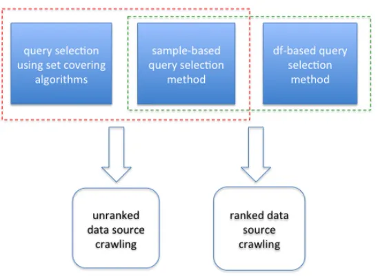
1.1 The key components in this dissertation for unranked and ranked deep web data sources. . . 4
2.1 An example from Amazon.com website . . . 12 2.2 The framework of form-focused crawling method . . . 14
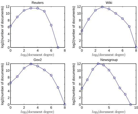
3.1 The illustration of the textual data source DB in Example 1. Each dot or circle represents one document or term, respectively. . . 21 3.2 The distribution of the document degrees using ’logarithmic binning’
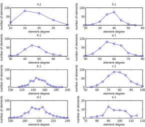
in log-log scale for our data sources. The bin size of the data increases in 2i (i= 1,2, . . .) . . . 30 3.3 The distributions of element degrees of part of the Beasley data. The
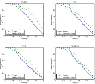
bin size is 5. . . 32 3.4 The results of all experiments on each corpus data with redundancy
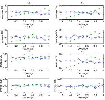
based on 100 runs. ’o’: the greedy method, ’.’: the weighted greedy method. . . 33 3.5 The average document degrees of the newly covered documents in
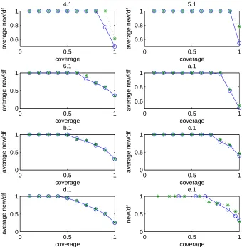
the greedy and weighted greedy query selection processes on our data sources. The bin size is 5%. . . 35 3.6 The average values of new/df in the greedy and weighted greedy
query selection processes on our corpus data sources. The bin size is 5%. . . 36 3.7 The average document frequencies of the selected documents in the
greedy and weighted greedy query selection processes on our data sources. The bin size is 5%. . . 37 3.8 The results of all experiments on Beasley data with redundancy. G:
the greedy method, W: the weighted greedy method. . . 40 3.9 The average document degrees of the newly covered documents in
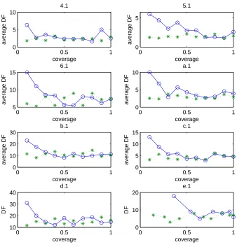
3.10 The average values of new/cost for each column in the greedy and weighted greedy query selection processes on parts of the Beasley data. The bin size is 10%. In subgraph e.1, the histogram is replaced with the scatter plot because some values of new/cost are zero and no column is selected in the corresponding coverage ranges. . . 43 3.11 The average document frequencies of selected columns in the greedy
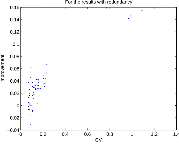
and weighted greedy query selection processes on part of Beasley data. The bin size is 10%. In subgraph e.1, the histogram is replaced with the scatter plot and the reason is same as Figure 3.10. . . 44 3.12 the relationship between the CV of document (element) degree and
the average of the improvement of the weighted greedy method on our and Beasley data with redundancy. . . 46
4.1 Our sampling-based query selection method. . . 52 4.2 Impact of sample size on HR projection. The queries are selected
fromDand cover above 99% of the documents inD. TheHRinDB
is obtained when those queries are sent to the original data source
DB. µ= 20. . . 59 4.3 Impact of sample size on OR projection. X axis is sample size, Y
axis is HR. Sample size is from 100 to 4,000 documents and µ= 20. 61 4.4 The impact of the sample size and the average document degree on
HR. . . 63 4.5 The impact of the sample size and the average document degree on
OR. . . 64 4.6 The impact of the value of the average document degree on OR
im-provement from the comparison between our and random methods for Reuters corpus. . . 66 4.7 Apply queries selected in one corpus to other corpora. Sample size
is 3,000, µ= 20. Each sub figure shows the querying results for the four data sources with the queries selected from one particular corpus. 68 4.8 Comparison with queries selected by using Ntoulas’ method. For
our method, the sample size is 3000, µ = 20 and the range of the sample document frequencies of the queries are between 2 and 500. For Ntoulas’ method, the stopping criterion is that no new document is returned after 10 consecutive queries sent. . . 70 4.9 Comparison with queries selected directly fromDB. Each sub figure
5.1 Scatter plots for the query results from different types of queries. For each experiment, 100 queries are sent. X axis represents the document rank and the return limit k = 20. Sub figure (A) queries withF = 40; (B) queries with 40≤F ≤80; (C) queries withF = 80. The data source is the Reuters. . . 75 5.2 The scatter plot for the query result. 100 queries whose F ≤ 20 are
sent and the return limit k= 20. . . 77 5.3 Our query selection method for ranked deep web data sources . . . 79 5.4 The trend of sample document frequency in Example 4 on log-log
scales. High sample document frequencies becomes horizontal along the line n1. . . 84
5.5 The smoothing result ofnf shown in Figure 5.4 for our SGT example
on log-log scales. Zf =
2nf
f′′−f′ and the line of best fity= 3.12−1.707×
log10(x) is obtained by using the least-squares curve fitting algorithm
provided in Matlab. . . 85 5.6 An artificial example to illustrate the basic idea of Ipeirotis’ estimator. 87 5.7 The example of the Zipf-law-based estimation method. . . 89 5.8 The average errors of the three estimators for the terms with 1 ≤
f ≤10 based on four different corpus samples. . . 93 5.9 The average of the document frequencies and the estimated
docu-ment frequencies of the three estimators for the low frequency terms based on four 3000-document samples. The MLE: the average of es-timated document frequencies from the MLE, the SGT: the average of estimated dfs from the SGT, Zipf: the average estimated dfs from the Zipf’s-law-based estimation. . . 94 5.10 The results of the three methods on different corpora. The return
limit k is 1000. Documents are statically ranked. MLE, SGT, Zipf: our methods with the MLE, the SGT and the Zipf-law-based estima-tion methods respectively. . . 97 5.11 The zoomed-in area of each subgraph in Figure 5.10. The range of
HR is up to 10%. . . 98
A.1 The results of all the experiments on each corpus data based on 100 runs. ’.’: greedy with redundancy, ’*’: weighted greedy with redundancy, ’o’: greedy without redundancy, ’+’: weighted greedy without redundancy. . . 111 A.2 Part of the results of all the experiments on the Beasley data based
A.3 The relationship between the CV of the document (element) degree and the average of the improvement of the weighted greedy method on our and the Beasley data without redundancy. . . 113
C.1 The probability mass functions of the document frequency of query
q with N = 1500 and p= 0.004(A) and p= 0.008(B) . . . 118 C.2 The likelihood function L(p|N, f(q)) with N = 1500 and f(q) = 12
Chapter 1
Introduction
The deep web [2] is the content that is dynamically generated from data sources
such as databases or file systems. Unlike the surface web, where pages are
col-lected by following the hyperlinks embedded inside colcol-lected pages, data from the
deep web are guarded by search interfaces such as HTML forms, web services, or programmable web API [3], and can be retrieved by queries only. The deep web
contains a much bigger amount of data than the surface web [4, 5]. This calls
for deep web crawlers to collect the data so that they can be used, indexed, and
searched in an integrated environment. With the proliferation of publicly available
web services that provide programmable interfaces, where input and output data
formats are explicitly specified, automated extraction of deep web data becomes
more practical.
Deep web crawling is the process of collecting data from search interfaces by
issuing queries. It has been studied from two perspectives. One is the study of the macroscopic views of the deep web, such as the number of the deep web data
sources [6, 4, 7], the shape of such data sources (e.g., the attributes in the HTML
form) [7], and the total number of pages in the deep web [2].
When crawling the deep web, which consists of tens of millions of HTML forms,
usually the focus is on the coverage of those data sources rather than exhaustively
crawling the content inside one specific data source [7]. That is, the breadth, rather
than the depth, of the deep web is preferred when the computing resource of a
crawler is limited. In this kind of breadth-oriented crawling, the challenges are
locating the data sources [8, 9, 10, 11], learning and understanding the interface
au-tomated [12, 11, 13, 14].
Another category of crawling is depth-oriented, focusing on one designated deep
web data source, with the goal to garner most of the documents from the given
data source [15, 16, 17, 7]. In this realm, the crucial problem is the query selection
problem, that is, to cover most of the documents in a specific data source with
minimal cost by submitting appropriate queries.
There are many existing works addressing the query selection problem [15, 16,
17, 18, 19, 20, 7] but still some issues remain as follows: 1) How to evaluate query selection algorithms; 2) How to optimize the query selection problem; 3) What the
input of query selection algorithms at beginning is; 4) How to crawl the deep web
data sources with return limit.
Based on the above issues, in this dissertation, we present a novel technique to
addressing the query selection problem. It contains three parts:
• Query selection using set covering algorithms: first we map the query selection problem to the set covering problem. If we let the set of documents in a data
source be the universe, each query represents the documents it matches, i.e.,
a subset of the universe. The query selection problem is thus cast as a set covering problem, and the goal is to cover all the documents with minimal
sum of the cardinalities of the queries.
Although set covering problem is well studied [21, 22, 23, 24] and numerous
algorithms even commercial products such as CPLEX [25] are available, the greedy algorithm remains the convenient choice for large set covering
prob-lems. A conventional greedy algorithm assigns the same weight to each
doc-ument, which may be good in other domains but not in our application. In
deep web data sources, one empirical law on the document size is that its
distribution is highly skewed, close to power law or log-normal distribution.
Many documents are of small size, while the existence of very large documents
cannot be neglected, so called long tail. Those large documents can be
cov-ered by many queries, therefore their importance or weight should be smaller.
We assign the reciprocal of the document size as the weight of a document,
and select the next best query accordingly.
We conducted experiments on a variety of test data, including the Beasley
deep web data sources. The results show that, with same time complexity, our
weighted greedy algorithm outperforms the greedy algorithm in both Beasley
and our data and, especially, for our data (heterogeneous data). Furthermore,
we argue that data distribution has a great impact on the performances of
the two greedy algorithms.
• Sampling-based query selection: before crawling the deep web, there is no input to the set covering algorithm, i.e., neither documents nor terms are available.
To bootstrap the process, a sample of the data source is needed so that some
good terms are selected and sent, and more documents are returned and added
to the input of the set covering problem. This repetitive and incremental process is used in the methods proposed by [17, 7]. The disadvantage is
the requirement of downloading and analyzing all the documents covered by
current queries to select the next query to be issued, which is highly inefficient.
We found that instead of incrementally running and selecting queries many
times, selecting all queries on a fixed sample at once is more efficient and
the result can be better as well. We first collect from the data source a set of documents as a sample that represents the original data source. From
the sample data, we select a set of queries that cover most of the sample
documents with a low cost. Then we use this set of queries to extract data
from the original data source. Finally, we show that the queries working well
on the sample will also induce satisfactory results on the original data source.
More precisely, the vocabulary learnt from the sample can cover most of the
original data source; the cost of our method in the sample can be projected to
the original data source; the size of the sample and the number of candidate
queries for our method do not need to be very large.
• Query selection for ranked data sources: many large data sources rank the matched documents and return only the top k documents, where k may be rather small ranging from 10 to 1000. For such ranked data sources, popular
queries will return only the documents in the top layers of the data.
Docu-ments ranked low may never be returned if only popular terms are used. In
order to crawl such data sources, we need to select the queries of appropriate
Figure 1.1: The key components in this dissertation for unranked and ranked deep web data sources.
of the small queries from a sample. In particular, the conventional Maximum
Likelihood Estimation [27] overestimates the rare queries. We use Simple
Good-Turing estimation [28] to correct the bias. Another estimation method
is based on Zipf’s law [29]. After a few probing queries issued for their
fre-quencies, the method tries to propagate the known frequencies to nearby terms
with similar frequencies.
The experimental result shows that crawling ranked data sources with small
queries is better than using random queries from a middle-sized Webster
En-glish dictionary, and much better than using popular terms as queries whose
frequencies are more than 2k.
Figure 1.1 shows the key components in our query selection technique for
un-ranked and un-ranked deep web data sources.
contain plain text documents only. These kinds of data sources usually provide a
single keyword-based query interface instead of multiple attributes, as studied by
Wu et al. [20]. Madhavan et al.’s study [7] shows that the vast majority of the
HTML forms found by Google deep web crawler contain only one search attribute,
thus we focus on such a search interface.
The rest of this dissertation is organized as follows: Chapter 2 introduces the
related work; in Chapter 3, we convert the query selection problem into set covering
problem and propose a weighted greedy algorithm to addressing it; Chapter 4 details our sampling-based crawling method; Chapter 5 shows our novel df-based crawling
method for crawling ranked deep web data sources; and finally Chapter 6 concludes
Chapter 2
Related work
In this chapter, we present a detailed introduction to the related work of our
re-search.
2.1
Query selection problem
The query selection problem is to select a set of queries to efficiently harvest a
specific deep web data source. There are many existing works addressing this
prob-lem [7, 15, 16, 17, 18, 19, 20].
A primitive solution could be randomly selecting some words from a dictionary.
However, this solution is not efficient because a large number of rare queries may
not match any page, or there could be many overlapping returns. Recently, instead
of selecting queries from a dictionary, several algorithms [17, 7, 15, 20, 16] have been
developed to select queries from the downloaded documents, which were retrieved by previous queries submitted to the target deep web data source.
Generally speaking, query selection methods can be categorized as: the methods
for unstructured data sources and the methods for structured data source.
2.1.1
Unstructured data sources
Here unstructured data sources refer to textual data sources that contain plain text
documents only. This kind of data sources usually provide a single keyword-based
query interface.
data sources. An incremental method selects queries from the downloaded
doc-uments and the number of docdoc-uments increases as more queries are sent. Their
method selects the query returning most new documents per unit cost iteratively
and it is represented by the formula Nnew(qj)
Cost(qj). For each query, its cost consists of
the costs for sending qj, retrieving the hyperlinks of the matched documents, and
downloading them.
Since there is no prior knowledge of all the actual document frequencies of the
queries in the original data source DB, this method requires the estimations of the actual document frequencies based on the documents already downloaded. With
the estimated document frequencies of all queries in the downloaded documents,
the number of matched new documents of each query will be calculated.
They proposed two approaches to estimate. The first method, called theindependence
estimator, assumes that the probability of a term in the downloaded documents is
equal to that in DB. Based on the document frequency of a term in the down-loaded documents N(qj|subset collection), the method can estimate how many
documents containing the term in the original data source Nb(qj). Then we can
es-timate the number of new returned documents by the equationNbnew(qj) =Nb(qj)−
N(qj|subset collection). The second estimation method is the Zipf-law-based
esti-mator provided in [29] (the detail of this method will be introduced in later section),
it estimates the actual document frequency of terms inside the document collection
by following Zipf’s law [30].
They compared their adaptive method with two other query selection methods:
the random method (queries are randomly selected from a dictionary), and the
generic-frequency method (queries are selected from a 5.5-million-web-page corpus
based on their decreasing frequencies). The experimental result shows that the
adaptive method performs remarkably well in all cases. However, their method
se-lects queries from an incremental document collection and it means that the method needs to analyze each document once it is downloaded and to estimate the document
frequency for every term inside it at each round. In order to estimate document
fre-quency efficiently, the solution from [17] computes the document frefre-quency of each
term by updating the query statistics table after more documents are downloaded.
But maintaining this table is still difficult.
Madhavan et al. [7] developed another incremental method for unstructured
how to select seed queries. Since they need to process difference languages, their
approach does not select queries from a dictionary. Instead, Their system detects
the feature of the HTML query form and selects the seed queries from it. After
that, the iterative probing and the query selection approach are similar to those,
that proposed in [17].
Their query selection policy is based on TF-IDF that is the popular measure
in the information retrieval. TF-IDF measures the importance of a word by the
formula below.
tf idf(w, p) = tf(w, p)×idf(w) (2.1)
tf(w, p) is the term frequency of the word w in any page p, and measures the importance of the word w in any page p.
tf(w, p) =nw,p/Np, (2.2)
where nw,p represents the number of times the wordw occurs in any pagep andNp
is the total number of the terms in any page p.
idf(w) (inverse document frequency) measures the importance of the word w
among all the web pages, and is calculated by log(dD
w) where D is the total number
of web pages and dw is the number of web pages where the term w appears.
Madhavan et al.’s method adds the top 25 words of every web page sorted by
their TF-IDF values into the query pool. From the query pool, they remove the
following two kinds of terms:
• Eliminate the high frequency terms, such as the terms that have appeared in many web pages (e.g., > 80%), since these terms could be from menus or advertisements;
• Delete the terms which occur only in one page, since many of these terms are meaningless words that are not from the contents of the web pages, such as
nonsensical or idiosyncratic words that could not be indexed by the search
engine;
The remaining words are issued to the target deep web data source as queries and
a new set of web pages are downloaded. Then this is repeated again in the new
Additionally, their approach emphasizes the breadth-oriented crawling that is
quite different to prior researches. They observed the statistical data on Google.com
and found that the results returned to users were more dependent on the number
of the deep web data sources. They analyzed 10 millions of deep web data sources.
They discovered that the top 10,000 deep web data sources accounted for 50% of the
deep web results, while even the top 100,000 deep web data sources only accounted
for 85%. This observation prompted them to their focus on crawling as many deep
web data sources as possible, rather than surfacing on a specific deep web data source.
In [16], Barbosa et al. proposed a sampling-based method to siphon the deep web
by selecting queries with highest frequencies from the sample document collection.
Unlike the incremental method, a sampling-based crawling method selects queries
from a fixed or near fixed sample which is usually derived from the first batch of
downloaded documents.
This method selects the highest frequency queries from the term list, which are
expected to lead a high coverage. It is composed of two phases: phase 1 selects a set
of terms from the HTML search form and randomly issues them to the target deep
web data source until at least a non-empty result page is returned. By extracting high frequency terms from the result pages, their algorithm creates a term list. Then
it iteratively updates the frequencies of the term and adds new high frequency terms
into the list by randomly issuing the term in the list until the number of submissions
reaches the threshold. In phase 2, the method uses a greedy strategy to construct a
Boolean query to reach the highest coverage, it iteratively selects the term with the
highest frequency from the term list, and adds it to a disjunctive query if it leads
to an increase in coverage. For example, if 10 terms (q1, . . . , q10) are selected, the
final issued disjunctive query is q1∨. . .∨q10.
The method is easy to implement but its shortcoming is obvious. Most of websites limit the number of the subqueries of a Boolean query and the number
of returned documents for a query. Thus using only one Boolean query to crawl a
2.1.2
Structured data source
A structured data source is a traditional relational database and all contents are
stored as records in tables. Usually the deep web site with a structured data source
provides a search interface with multiple attributes instead of a single
keyword-based search bar.
Wu et al. [20] presented a graph-based crawling method to retrieve the data
inside a specific deep web data source. In their method, a structured data source
DB is viewed as a single relational table with ndata records {t1, . . . , tn}over a set
of m attributes {attr1, . . . , attrm}. All distinct attribute values are contained by
the Distinct Attribute Value set (DAV).
Based on a data sourceDB, an attribute-valueundirected graph (AV G) can be constructed. Each vertex vi represents a distinct attribute value avi ∈ DAV and
each edge (vi, vj) stands for the coexist of the two attribute valuesavi andavj in a
record tk.
According to AV G, the process of crawling is transformed into a graph traver-sal in which the crawler starts with a set of seed vertices and at each iteration a
previously seen vertex v is selected to visit, thus all directly-connected new vertices and the records containing them are discovered and stored for future visits.
Raghavan et al. [15] proposed a task-specific human-assisted crawling method for
structured data sources. First, it needs a task-specific database D which contains enough terms for the crawler to formulate search queries relevant to a particular
task. For example, to retrieve documents about semiconductor industry in a data
source DB, D should contain the lists of semiconductor companies and product names that are of interest. For the query selection strategy, the authors assume
that all attributes are independent from each other, and all records can be retrieved
by using the Cartesian product of all possible attribute values from the task-specific
database D.
Namely, for each attributeEishown in the multi-attribute search form, a
match-ing function is used to assign a value shown in Equation 2.3.
M atch(({E1, . . . , Em}, S, M), D) = [E1 =v1, . . . , Em =vm] (2.3)
where {E1, . . . , Em} is a set of m form attributes, S is the submission
infor-mation about the form (e.g., the URL of the form page). A value assignment
[E1 =v1, . . . , Em =vm] associates value vi with form attribute Ei and the crawler
uses each possible value assignment to ’fill-out’ and submit the completed form.
This process is repeated until the set of value assignments is exhausted.
In Raghavan et al.’s method, the product of all possible attribute values could
be a large number and sometimes it means a high communication cost and an empty
return result, which could significantly reduce the effectiveness and efficiency of the
crawler.
2.2
Automated form filling
Before the query generation process, the problem of how to automatically interact
with the search interface has to be addressed firstly.
For the deep web crawling, the automated form filling is simpler than other
techniques such as the virtual data integration [31, 32, 33] and the web information
extraction [34, 35, 19, 36], which need to deal with semantic inputs based on a
given knowledge. Here the technique of form filling used by Google’s deep web crawling [7] is presented as an example.
In Google’s deep web crawling [7], they only focuses on two kinds of inputs
in a searchable form. One is the selection input that offers users some imposed
items to choose, such as the select menu, the radio button and the check box; the
other one is the free input, e.g., the text box. A selection input often provides a
default item, if it is not selected as a certain value, the effect of the input for search
results can be ignored. Among the selection inputs, there exists a special ordering
input which arranges the returned results according to an order. A crawler has
to distinguish the ordering input from other kinds of selection inputs because such the ordering input causes a much overlapping retrieval. The free input could be
anywhere, usually called a search bar. It accepts any keyword (or Boolean query)
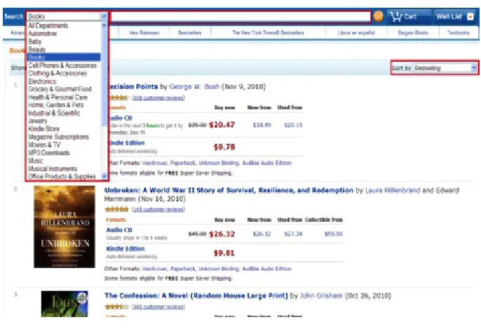
and returns documents containing the keyword. Figure 2.1 shows an example of the
two kinds of inputs from the website of Amazon.com. In the figure, two selection
inputs (drop-down menus) are on the left and right sides respectively. The right
one is an ordering input, and a free input (text box) lies in the center.
Figure 2.1: An example from Amazon.com website
can be described as following:
select K f rom DB where P ordered by O.
where K = (keyword1, ..., keywordn), P = (constrain1 = c1, ..., constrainm =cm),
and O = orderi. Each keyword is from a free input, each constrain is set by the
selection input one by one and the return order is decided by the value of the order
selection input.
Recognizing free inputs and selection inputs, it can be done easily by analyz-ing the HTML code of the form pages. In [7], the free input of a search form is
automatically filled out by selecting queries from the query list derived from the
retrieved document collection. Each selection input and its value are decided by
the informativeness test that is used to evaluate query template, i.e., the
combina-tions of the selection inputs. The basic idea of the informativeness test is that all
templates (the searchable form with different values for each selection input) are
probed to check which can return sufficiently distinct documents. A template that
2.3
Automated searchable form discovery
Before crawling the deep web data sources, first of all, we have to locate the
en-trances (searchable forms) of the targeted data sources. It is a challenging problem
due to several reasons. Firstly, the contents in the Web keep changing at all time;
it is continually updating the routine, adding new websites, and removing old ones.
In addition, the entrances of these data sources are sparsely distributed on the Web. Thus, to acquire a few deep website locations, a surface web crawler needs to search
tons of useless web pages and this could consume the resources of the crawler too
much.
Note that a crawler for the surface web is quite different from the one for the deep
web. The former usually starts at some seed web pages and follows all the outgoing
hyperlinks of the visited web pages to traverse the linked pages, and this iterative
process ends when all the reachable web pages are visited or the stopping criteria
are satisfied. The latter works on the many searchable forms of the backend data
sources by issuing queries and retrieving all the returned documents. The crawler for locating the entrances of deep web data sources is the one for the surface web.
At the beginning, an exhaustive crawler is used to crawl all the web pages it can
reach to find the entrances (such as the crawlers Alta Vista, Scooter, and Inktomi).
The whole process could take a few of weeks up to months. However, owing to the
rapid increase of the Web, it becomes harder and harder to implement.
In common, users prefer a collection of searchable forms that can return high
relevant documents. Hence, some researchers [10, 37] provided the concept of
fo-cused crawler that it is a topic-driven crawler. A fofo-cused crawler tries to retrieve
a subset of web pages from the surface web that are highly relevant to a topic so
that related searchable forms are likely contained in this collection.
In [10], the surface web is considered a directed graph G given a predefined hierarchy tree-structured classification C on topics, such as Yahoo!. Each node
c∈C refers to some web pages inGas examples denoted asD(c). A user’s interest can be characterized by a subset of topicsC∗ ⊂C. Given any web pagep, a method is used to calculate the relevant value RC∗(p) for p with respecting to C∗. Based
on the relevant value of p , its neighbour web pages (directly linked by p) firstly estimates relevant values, and, after crawled, the estimated relevant values of the
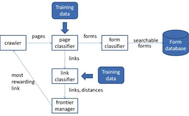
Figure 2.2: The framework of form-focused crawling method
The crawling process starts from example web pages D(C∗). At each iteration, the crawler inspects the current set V of the visited web pages and then selects an unvisited web pages corresponding to the hyperlinks in one or more visited web
pages by their estimated relevant values.
Focused crawlers can significantly reduce the number of useless web pages crawled
but the ratio between the number of forms and the number of visited pages is still
low. In a recent search work in [11], the authors provide a Form-Focused
Crawl-ing(FFC) method to seek the searchable forms based on topics. The difference is
that the previous focused crawler focuses the search process based solely on the
contents of the retrieved pages, and it is not enough. FFC combines the techniques
of the previous focused crawlers with a link classifier that analyzes and prioritizes
the links that will likely lead to searchable forms in one or more steps. Figure 2.2
shows the framework of the form-focused crawling method.
In this figure, there are four major parts in the framework: page classifier, link classifier, frontier manager, and form classifier. The page classifier is trained to
identify the topic of the crawled web pages and it uses this strategy in [10]. The
searchable form classifier is used to filter out non-searchable forms.
The link classifier and the frontier manager are highlight parts. The authors
are likely to lead to a searchable form in one or more steps. The backward search
method starts with a given set of URLs of web pages that contain forms in a
specified domain. Links to these pages are acquired by crawling backward from
these pages based on the facilities from standard search engines, such as Google
and Yahoo! [38]. The process of backward crawling is breadth-oriented, and all the
retrieved documents in levell+1 are linked to at least one of the retrieved documents in level l. At each iteration, the best features of the links in the corresponding level are manually collected. Finally, those features are used to train the link classifier to estimate the steps from a given link to a searchable form.
In the frontier manager, there are multiple priority queues for the links that are
not visited, and each queue corresponds to a certain estimated step given by the
link classifier. It means that a link l is placed in the queue i if the link l has i
estimated steps to the target searchable form. At each crawling step, the manager
selects the link with the maximum reward value as the next crawling target, and
the reward for a link is decided by the current status of the crawler and the priority
of the link.
There are still a few of other methods used to locate searchable forms (e.g., IP
sampling method). However, as far as we know, they do not address this problem well.
2.4
Sampling techniques
Query selection is based on various properties of the data source, such as the df
of all the terms. However, such resource descriptions are not provided by most of
deep web sites. They need to be leant by sample. To select appropriate queries for crawling, random sampling methods [1, 39, 40] become an important way to acquire
the resource description of a target data source and such information usually is the
basis of most of query selection methods.
In [1], the authors provided a query-based sampling method for textual deep
web data sources and showed that their method can efficiently acquire the accurate
term frequency list of the target data source based on a sufficiently unbiased sample.
Their query-based sampling algorithm is shown as follows:
docu-Table 2.1: The consistency between the conclusions of Callan’s work [1] and our sampling-based query selection method
No. Callan’s conclusion Our conclusion 1. sample can contain most of the
common terms in the originalDB
selected queries from sample can cover most of the original DB. 2. the rank list of terms in the
sam-ple can represent the order of the corresponding terms in the origi-nal DB in a way
selected queries from the sample can cover most of the originalDB
with low cost.
3. small sample can capture most of the vocabulary and the rank in-formation of the original DB
to harvest most of the original
DB, the sample size and the query pool size do not need to be very large.
2. Send the selected query to the target data source and retrieve the top k
documents;
3. Update the resource description based on the characteristics of the retrieved
documents (extract terms and their frequencies from the topkdocuments and add them to the learned resource description);
4. If the stopping criterion has not yet been reached, select a new query and go
to Step 2
The above algorithm more looks more like a framework and some parameters
need to be decided. What is the best value for N? How to select an initial query? How to select a term as query for further retrieval? What is the stopping criterion?
All those questions are answered in [1].
The conclusions of the Callan’s sampling method support our sampling-based
query selection method in Chapter 4 and they are indirectly verified by our results.
The corresponding relationship is shown in Table 2.1.
In [40], the authors presented a Boolean query-based sampling method for the
sampling of uniform documents from a search engine’s corpus. The algorithm
for-mulates ”random” queries by using disjunctive and conjunctive Boolean queries to
pick uniformly chosen documents from returned results. The method needs the
frequency on the Web. The lexicon is generated in a preprocess by crawling a large
corpus of documents from the Web.
The method [40] is somehow the reverse process of the deep web crawling. For
the crawling process, a random sample is needed first and then it begins based on
the terms inside the sample, but this method first requires the crawling results that
help to do the random sampling.
In [39], the authors proposed two elaborate random sampling methods for a
search engine corpus. One is the lexicon-based method and the other is the random walk method. Both methods produce biased samples and each sample is given a
weight to represent its bias. Finally, all samples in conjunction with the weights,
applied using stochastic simulation methods, are considered a near-uniform sample.
Compared to the methods in [1, 40], this method performs better but its complexity
Chapter 3
Query selection using set covering
algorithms
3.1
Introduction
In this and the next chapter, we discuss the query selection problem for deep web
data sources without a return limit, i.e., all documents matched by a query should
be returned. We focus on such data source first because
• there are many such data sources in the Web, especially the websites for public services, such as the PubMed website [41] or the website of United
States Patent and Trademark Office (USPTO) [42];
• the strategies of the query selection for data sources without a return limit can provide an insight to the one with a return limit (we will discuss the latter
in Chapter 5).
Let the set of documents in a data source be the universe. If one term is
contained by one document, we say that the term coversthis document. The query
selection problem is to find a set of terms as queries which can jointly cover the
universe with a minimal cost. Thus, it is cast as a set covering problem (SCP). SCP is an NP-hard problem [43] and has been extensively studied by many
researchers [21, 22, 23, 24] in fields such as scheduling problem, routing problem,
Many algorithms have been developed for set covering problem. Some of them,
such as [44, 45, 46], can provide better solutions in general but require more
re-sources for the execution. For example, since the Optimization Toolbox for binary
integer programming problems provided by Matlab can only work within 1G
mem-ory limit [47], it is easy to be out of memmem-ory for one thousand by thousand input
matrix.
Based on the above consideration, the greedy method is a better choice because
it usually leads to one of the most practical and efficient set covering algorithms. But we found that, so far, most of the research work on greedy methods have been carried
out on the normally distributed data and the corresponding results are acceptable
compared with the optimal solutions (or the best known solutions). In deep web
crawling, the degrees of the documents are not distributed normally. Instead, they
follows a lognormal distribution. For data with a lognormal distribution, the results
of the greedy method could be improved.
We have developed a weighted greedy set covering algorithm. Unlike the greedy
method, it introduces weights to the greedy strategy. We differentiate among
doc-uments according to the dispersion of document degree caused by the lognormal
distribution. A document with a smaller document degree is given a higher docu-ment weight. A docudocu-ment with a higher weight should usually be retrieved earlier
since it will lower the total cost in the future. This is combined with the existing
greedy strategy. Our experiment carried out on a variety of corpora shows that the
new method outperforms the greedy method when applied on data with a lognormal
distribution.
After analyzing the greedy and our weighted greedy methods on data with
var-ious distributions, we further argue that the data distribution plays a great role in
the performances of the two greedy algorithms.
3.2
Set covering
The query selection problem is to find a set of terms as queries which can jointly
cover the universe with a minimal cost. The query cost is defined by a number of
factors, including the cost for submitting the query, retrieving the URLs of matched
documents from resulting pages, and downloading actual documents. There is no
a given query, there could be many matched documents and they are returned
in the resulting pages instead of in a long list. Thus the number of queries is
proportional to the total number of retrieved documents because the same query
needs to be sent out repeatedly to retrieve the subsequent pages. For example, if
there are 1,000 matches, the data source may return one page that consists of only
10 documents. If you want the next 10 documents, a second query needs to be sent.
Hence, to retrieve all the 1,000 matches, altogether 100 queries with the same term
are required.
The cost of downloading actual documents should be separated from the cost
in the query selection problem. Since no one will repeatedly download redundant
documents, the cost of downloading all the documents of a data source is a constant.
Thus it does not help to find out a set of appropriate queries to submit by measuring
their downloading cost.
In this setting, we argue that the cost of retrieving the URLs of matched
docu-ments is the cost to consider for the query selection problem, and it can be
repre-sented by the total sum of the document frequencies of the selected queries.
Given a set of documents D={d1, ..., dm} and a set of termsQP ={q1, ..., qn},
their relationship can be represented by the well known document-term Matrix
A = (aij) whereaij = 1 if the documentdi contains the term qj; otherwise aij = 0.
The query selection problem can be modeled as set covering problem defined
in [43].
Definition 1 (SCP)Given an m×nbinary matrix A= (aij), letC = (c1, . . . , cn)
be a non-negative n-vector and each cj = m
∑
i=1
aij represents the cost of the column j.
SCP calls for a binary n-vectorX = (x1, . . . , xn)that satisfies the objective function
Z =min
n
∑
j=1
cjxj. (3.1)
Subject to
n
∑
j=1
aijxj ≥1, (1≤i≤m). (3.2)
xj ∈ {0,1}, (1≤j ≤n). (3.3)
Figure 3.1: The illustration of the textual data source DB in Example 1. Each dot or circle represents one document or term, respectively.
term in the query pool QP and each row represents a document ofDB. cj = m
∑
i=1
aij
is the document frequency (df for short) of the termqj, which is equal to the number
of documents containing the term. We should be aware that the terms in the QP
of a data source are usually parts of all the terms inside the data source; otherwise,
there could be more than millions of terms in the QP and it would be out of the capability of most set covering algorithms.
Example 1 Given a deep web textual data source DB = {d1, ..., d9} shown in
Figure 3.1, there are 5 terms (QueryP ool = {q1, ..., q5}) and each is contained in
at least one of the 9 documents. For example, d1 contains q3 only, and d2 contains
q3 and q4. The doc-term matrix representation of the data source is shown in
Table 3.1. The optimal solution of SCP here is {q4, q3, q1} (with corresponding
Table 3.1: The doc-term Matrix A in Example 1
q1 q2 q3 q4 q5
d1 0 0 1 0 0
d2 0 0 1 1 0
d3 1 0 1 0 1
d4 0 0 1 0 1
d5 1 0 0 0 1
d6 1 1 0 1 0
d7 0 0 0 1 0
d8 1 1 0 0 1
d9 0 0 1 1 1
df 4 2 5 4 5
3.3
Greedy algorithm
The basic idea of the greedy algorithm [48] is to construct a solution in a step-by-step
manner and to approximate a global optimal solution by choosing alocally optimal
solution on each step. For a set covering problem, the solution is constructed
step-by-step: on each step, one column is selected as a part of solution until the
requirement is reached.
There are various ways to select a column.
• Minimize cost: we can select the next column qu which has the lowest cost
on this step, namely, cu = min(cj) where 1 ≤j ≤ n and xj = 0. The lowest
total cost
n
∑
j=1
cjxj is approximated by having the smallest cost on each step;
• Maximize coverage: another popular way is to select the next columnqu which
can cover the largest number of rows that are not yet covered by the previously
selected columns, namely, settingxu = 1 to maximize m
∑
i=1
((1−yi)×aiu) where
yi ∈ {0,1} and yi = 1 if di have been covered, otherwise,yi = 0. Such a local
optimization aims at reaching the expected coverage in fewer steps so that
the number of selected columns can be kept small. In this way, the total cost
n
∑
j=1
cjxj can get close to the smallest. This approach is especially suitable
when all columns in MatrixA have the same cost, and the total cost is purely determined by the number of selected columns.
is selected taking into account both its cost (cu) and the number of new rows that
can be covered (
m
∑
i=1
((1−yi)×aiu)). One of the possible combinations is described
as Algorithm 1 based on Definition 1. In the following, we use new/cost to denote
the value for local query selection. In this algorithm, yi = 1 indicates that the i-th
Algorithm 1: Greedy algorithm.
Input: an m×n matrix A = (aij)
Output: a solution n-vector X = (x1, . . . , xn)
Process: 1 cj =
m
∑
i=1
aij; xj = 0(1≤j ≤n);yi = 0(1≤i≤m);
2 while(
m
∑
i=1
yi < m){
3 find a column qu which maximizes m
∑
i=1
((1−yi)×aiu)/cu;
4 xu = 1; yi = 1 if n
∑
j=1
aijxj ≥1;
5 }
document is already covered.
Ostensibly, the greedy strategy is faultless but there are still some problems we
need to discuss and such problems may lead to an insight to the potential shortage.
3.4
Introducing weight to greedy algorithm
With the step-by-step manner, different rows are covered in different steps. Is there
any difference to covering a row earlier or later? In the above greedy strategy, all
newly covered rows are always considered as having a unit cost and there is no difference whether they are covered earlier or later.
In Table 3.1, the rows d1 and d7 are only covered by the columns q3 and q4
respectively. Such documents should be covered as early as possible. To easily
compare, let’s say thatq4 is set to the initially selected column and then the unique
solution from the greedy algorithm is {q4, q5, q3} with the cost 14. Actually, the
optimal solution is {q4, q3, q1} with the cost 13, and this optimal solution can be
find an optimal solution in this case is not to consider covering d1 and d7 by using
q3 and q4 as early as possible.
Now that we know there is a difference in covering certain rows earlier or later,
the second question is how to measure such difference to cover a row earlier or later.
For each row i, we argue that if the number of the columns covering row iis bigger, it is better to be covered later. Here are two reasons:
• When row i is covered at high coverage (in later steps) and most of the rows are already covered, more columns covering row i mean that there could be more possibilities to select a small-cost column which covers few new rows (of
course, at high coverage, no column can take many new rows);
• When rowi is covered at low coverage (in earlier steps) and most of the rows are not covered yet, more columns covering row i mean that there are more possibilities to cause overlapped coverage, i.e., row i will be covered many times.
For each document, we call the number of the terms in the query pool QP
covering it the degree of the document. Based on the above intuition, a higher
degree of a document means that the document needs to be covered later. It is
defined as follows:
Definition 2 (document degree) The degree of a document (element) di in DB
with respect to QP, denoted by deg(i), is the number of different terms in QP that occur in the document di, i.e.,
deg(i) =
n
∑
j=1
aij. (3.4)
Then we define dw(i) as document weight by using the document degree as follows:
Definition 3 (document weight) The weight of a document di in DB with
re-spect to QP, denoted by dw(i) (or dw for short), is the inverse of its document degree, i.e.,
dw(i) = 1
Intuitively, the fewer the terms (columns) are contained in documentdi (rowi),
the larger the weight that is given to it.
After all, covering rows is implemented by selecting columns one by one. At
each step, the column covering the rows with larger weights should be selected
earlier. Based on the definition of the document weight, for each term (column)
qj at each step, we sum up all weights of uncovered documents (rows) covered by
it and obtain the query weight qw for the term (column) qj. The terms (columns)
with larger weights should be selected as early as possible.
Definition 4 (query weight) The weight of a query qj (1≤ j ≤n) in QP with
respect to DB, denoted by qw(j) (or qw for short), is the sum of the document weights of all the uncovered documents containing the term qj, i.e.,
qw(j) =
m
∑
i=1
(aij ×dw(i)×(1−yi)), (3.6)
where (aij) is the corresponding Matrix A and yi = 1 if di has been covered,
other-wise, yi = 0.
3.4.1
Weighted algorithm
We consider qw(j) a better measurement than new(j) as it combines both the
in-formation about how many new documents can be obtained by selecting query qj
and the information about how soon the newly obtained documents should be
con-sidered to be covered. Consequently, we use qw/cost to replace new/costfor query
selection. We call the corresponding algorithm weighted greedy algorithm.
Based on the definitions of the document weight and the query weight, we
present our weighted greedy algorithm shown in Algorithm 2.
Example 2 Based on the matrix in Table 3.1, the initial weights of the documents
and the queries are shown in Table 3.2. In the first round of Algorithm 2, row q4
has the maximum value of qw/cost (0.54). It is selected as the first query, hence the corresponding x4 is set to 1. For convenient to explanation, the column q4 and
the covered rows, i.e., d2, d6, d7 and d9 are removed from the matrix A, and the
Algorithm 2: Weighted greedy algorithm.
Input: an m×n matrix A = (aij)
Output: a solution n-vector X = (x1, ..., xn)
Process: 1 cj =
m
∑
i=1
aij; xj = 0(1≤j ≤n);yi = 0(1≤i≤m);
2 while(
m
∑
i=1
yi < m){
3 find a column qu that maximizesqw(u)/cu;
4 xu = 1; yi = 1 if n
∑
j=1
aijxj ≥1;
5 }
Table 3.2: The initial weight table of Example 2 corresponding to Matrix A
t1 t2 t3 t4 t5
d1 0 0 1 0 0
d2 0 0 0.5 0.5 0
d3 0.33 0 0.33 0 0.33
d4 0 0 0.5 0 0.5
d5 0.5 0 0 0 0.5
d6 0.33 0.33 0 0.33 0
d7 0 0 0 1 0
d8 0.33 0.33 0 0 0.33
d9 0 0 0.33 0.33 0.33
cost(df) 4 2 5 4 5
qw 1.49 0.66 2.66 2.16 1.99
qw/cost 0.37 0.33 0.53 0.54 0.39
third rounds, q3 and q1 are selected respectively and the solution of the weighted
greedy is X = (1,0,1,1,0), and its cost is 13(4+5+4).
3.4.2
Redundancy removal
A solution generated from the above two methods could usually contain redundancy,
i.e., although some columns from the solution are removed, it can still cover all the
rows of matrixA. Here, if a solution does not contain any redundancy, it is a prime
Table 3.3: The second-round weight table of Example 2
t1 t2 t3 t5
d1 0 0 1 0
d3 0.33 0 0.33 0.33
d4 0 0 0.5 0.5
d5 0.5 0 0 0.5
d8 0.33 0.33 0 0.33
cost(df) 4 2 5 5
qw 1.16 0.33 1.83 1.66
qw/cost 0.29 0.165 0.36 0.33
X without it is still a solution, the corresponding xj is set to 0. When all the
selected columns of X have been considered, the derived solution X becomes a prime solution.
Algorithm 3: Redundancy removal algorithm.
Input: an m×n matrix A = (aij), a solution n-vector X = (x1, ..., xn)
Output: a prime solution X = (x1, ..., xn)
Process:
1 foreachxu = 1 (1≤u≤n)
2 setxu = 0 if∀i, ( u∑−1
j=1
aijxj+ n
∑
j=u+1
aijxj)≥1;
3.5
Experiments and analysis
3.5.1
Experimental setup
The purpose of the experiment is to test whether the weighted greedy is better than
the greedy algorithm in terms of the solution results. Note that the performances
of the two algorithms are similar since they are both greedy algorithms.
On the same input matrix, the greedy algorithm may produce different solutions
because in each step, especially in the initial stage, there are ties to select from. In
our implementation, we randomly selected one of the candidates when ties occurred.
Therefore, the solution values of the same input fluctuate with each run.
average cost (avg) and the standard deviation of the costs (SD). More specifically,
given the results C1, C2, . . . , C100, the average and standard deviation of the results
are defined as follows:
SD =
v u u t
n
∑
i=1
(Ci −avg)2
n ,
where avg =
n
∑
i=1
cj
n and n = 100.
The improvement of the weighted greedy algorithm can be calculated by using
the formula
IM P = Cg−Cw
Cg
.
where Cg and Cw are the results from the greedy and weighted greedy algorithms
with the same characteristics, such as the average, maximum, and minimal results.
For example, for calculating the average improvement, Cg and Cw should be the
average costs from the greedy and weighted greedy algorithms.
3.5.2
Data
The experiment was carried out on two different sets of data. One is derived from
the deep web crawling problem, and the other is from the Beasley data that are the
standard benchmarks for set covering problems [26].
For the data in deep web crawling problem, we experimented with four data
collections that cover a variety of forms of web data, including
• regular web pages (web pages under .gov domain),
• web articles (articles in wikipedia.com),
• newspaper articles (from Reuters),
• newsgroup posts in newsgroups.
We experimented with these data in order to show that our algorithm performs consistently across domains, and is independent of the forms of the web documents.
Although each data collection is huge, in the size of millions or more, we report
only the results on subsets of the documents that contain ten thousand documents.