Image Mining for Leaf Classification to detect
belonging tree by Association Reverse Rule
Using Texture features
Aswini Kumar Mohanty, Amalendu Bag
Principal, KMBB College of Engg & CET, Bhubaneswar, Orissa, India
Assistant Professor, Department of Computer Science, KMBB College of Engg & CET, Bhubaneswar, Orissa, India
ABSTRACT: The image mining technique deals with the extraction of implicit knowledge and image with data relationship or other patterns not explicitly stored in the images. It is an extension of data mining to image domain. Textures are one of the basic features in visual searching, computational vision and also a general property of any surface having ambiguity. The main objective of this paper is to apply image mining in the domain such as different leaves belonging to different trees to classify and detect the exact belonging class of tree. Leaf images of different trees with different texture and shape including sizes can be classified into many classes as per given data base and to explore the feasibility of data mining approach. Results will show that there is promise in image mining based on content. It is well known that data mining techniques are more suitable to larger databases than the one used for these preliminary tests. In particular, a Computer aided method based on association rules becomes more accurate with a larger dataset. Traditional association rule algorithms adopt an iterative method to discovery frequent item set, which requires very large calculations and a complicated transaction process. Because of this, a new association rule algorithm is proposed in this paper. Experimental results show that this new method can quickly discover frequent item sets and effectively mine potential association rules. A total of 26 features including histogram intensity features and GLCM features are extracted from leaf images. Experiments have been taken for a data set of 322 images taken of different types with the aim of improving the accuracy by generating minimum no. of rules to cover more patterns. The accuracy obtained by this method is approximately 97% which is highly encouraging.
KEYWORDS: Mammogram, Gray Level Co-occurrence Matrix feature, Histogram Intensity, Contrast Limited Adaptive Histogram Equalization Association rule mining, Reverse Rule Generation algorithm.
I. INTRODUCTION
Leaf recognition is a pattern recognition task performed specifically on leaves. It can be described as classifying a leaf either "known" or "unknown", after comparing it with stored known leaves. It is also desirable to have a system that has the ability of learning to recognize unknown leaves. Computational models of leaf recognition must address several difficult problems. This difficulty arises from the fact that leaves must be represented in a way that best utilizes the available leaf information to distinguish a particular leaf from all other leaves.
.
Compared with other methods, such as cell and molecule biology methods, classification based on leaf image is the first choice for plant classification. Sampling leaves and photogenic them are low-cost and convenient. One can easily transfer the leaf image to a computer and a computer can extract features automatically in image processing techniques. Some systems employ descriptions used by botanists. But it is not easy to extract and transfer those features to a computer automatically.
.
Data mining of texture images is used to collect effective models, relations, rules, abnormalities and patterns from large volume of data. This procedure can accelerate the classification process and decision-making. Different methods of data mining have been used to detect and classify anomalies in mammogram images such as wavelets [4,5], statistical methods and most of them used feature extracted using image processing techniques [6].Some other methods are based on fuzzy theory [7,8] and neural networks [9]. In this paper we have used classification method called Association classifier for image classification [10-12].
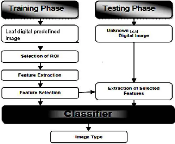
Classification process typically involves two phases: training phase and testing phase. In training phase the properties of typical image features are isolated and based on this training class is created .In the subsequent testing phase , these feature space partitions are used to classify the image. A block diagram of the method is shown in figure1.
Fig. 1.: Block diagram for Leaf classification system
II. METHODOLOGY 2.(a) Digital leaf database
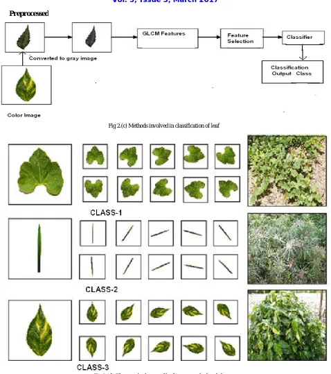
The database used in our experiment is collected by our self. We pluck the leaf from the plant in the fields near by surroundings and around the college campus, which consists of intact and fresh leaf images in different rotation for 3 plant species class and constructed by our self. We have taken total 322 images as whole. Each plant class contains around 100 leaf images in different degree of rotation and different leaf images. The test set contains the 114 of deformed and new leaf images and for each class has 38 leaf images for test. The sample dataset of leaf images and related classes are illustrated in Figure 2(d)..
Fig 2.(c) Methods involved in classification of leaf
Fig 2 (d). The sample dataset of leaf images and related classes
2..(b) Pre-processing
Since the leaf image for this study is taken by photographic camera and is converted from RGB to gray scale, it may contain some noise which could do difficulty to interpret. Therefore preprocessing is necessary to improve the quality of image and make the feature extraction phase as an easier and reliable one. The gray image of leaf before preprocessing is
shown in figure2.(a). .A pre-processing; usually noise-reducing step [13, 14] is applied to improve image and contrast figure 2.(b). Histogram equalization is a method in image processing of contrast adjustment using the image's histogram [17]. Through this adjustment, the intensities can be better distributed on the histogram. This allows for areas of lower local contrast to get better contrast. Histogram equalization accomplishes this by efficiently spreading out the most frequent intensity values. The method is useful in images with backgrounds and foregrounds that are both bright or both dark. In particular, the method can lead to better views of bone structure in x-ray images, and to better detail in photographs that are over or under-exposed. In mammogram images Histogram equalization is used to make contrast adjustment so that the image abnormalities will be better visible In this work the efficient filter (CLAHE) was applied..Contrast limited adaptive histogram equalization (CLAHE) method seeks to reduce the noise produced in homogeneous areas and was originally developed for medical imaging [15]. This method has been used for enhancement to remove the noise in the pre-processing of digital images [16]. CLAHE operates on small regions in the image called tiles rather than the entire image. Each tile’s contrast is enhanced, so that the histogram of the output region approximately matches the uniform distribution or Rayleigh distribution or exponential distribution. Distribution is the desired histogram shape for the image tiles. The neighboring tiles are then combined using bilinear interpolation to eliminate artificially induced boundaries. The contrast, especially in homogeneous areas, can be limited to avoid amplifying any noise that might be present in the image.
Fig 2.(a). Before preprocessing Fig2.(b) After Pre-processing Operation
III. FEATUREEXTRACTION
Features, characteristics of the objects of interest, if selected carefully are representative of the maximum relevant information that the image has to offer for a complete characterization a lesion [18, 19]. Feature extraction methodologies analyze objects and images to extract the most prominent features that are representative of the various classes of objects. Features are used as inputs to classifiers that assign them to the class that they represent. In this Work intensity histogram features and Gray Level Co-Occurrence Matrix (GLCM) features are extracted.
3.(a) intensity histogram features
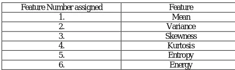
Intensity Histogram analysis has been extensively researched in the initial stages of development of this algorithm [18, 20]. Prior studies have yielded the intensity histogram features like mean, variance, entropy etc. These are summarized in Table 3.1. Table 3.2 summarizes the values for those features.
Table 3.1: Intensity histogram features
Feature Number assigned Feature
1. Mean
2. Variance
3. Skewness
4. Kurtosis
5. Entropy
6. Energy
Table 3.2: Intensity histogram features and their values
Image Type Features
Mean Variance Skewness Kurtosis Entropy Energy normal 7.2534 1.6909 -1.4745 7.8097 0.2504 1.5152 malignant 6.8175 4.0981 -1.3672 4.7321 0.1904 1.5555 benign 5.6279 3.1830 -1.4769 4.9638 0.2682 1.5690
3.(b) glcm features
It is a statistical method that considers the spatial relationship of pixels is the gray-level co-occurrence matrix (GLCM), also known as the gray-level spatial dependence matrix [21, 22, 23, 24]. By default, the spatial relationship is defined as the pixel of interest and the pixel to its immediate right (horizontally adjacent), but you can specify other spatial relationships between the two pixels. Each element (I, J) in the resultant GLCM is simply the sum of the number of times that the pixel with value I occurred in the specified spatial relationship to a pixel with value J in the input image.
3.2.(c) glcm construction
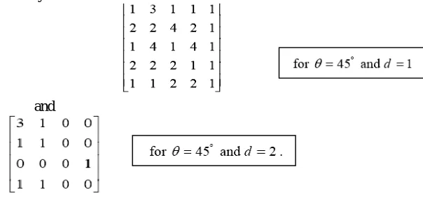
GLCM is a matrix S that contains the relative frequencies with two pixels: one with gray level value i and the other with gray level j-separated by distance d at a certain angle θ occurring in the image. Given an image window W(x, y,
c), for each discrete values of d and θ, the GLCM matrix S(i, j, d, θ) is defined as follows.
An entry in the matrix S gives the number of times that gray level i is oriented with respect to gray level j such that W(x1, y1)=i and W(x2, y2)=j, then
We use two different distances d={1, 2} and three different angles θ={0°, 45°, 90°}. Here, angle representation is taken
in clock wise direction. Example
Intensity matrix
and
The Following GLCM features were extracted in our research work:
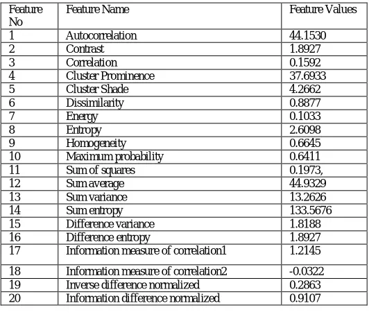
Table 3.3 : GLCM Features and values Extracted from a sample leaf image
Feature No
Feature Name Feature Values
1 Autocorrelation 44.1530
2 Contrast 1.8927
3 Correlation 0.1592
4 Cluster Prominence 37.6933
5 Cluster Shade 4.2662
6 Dissimilarity 0.8877
7 Energy 0.1033
8 Entropy 2.6098
9 Homogeneity 0.6645
10 Maximum probability 0.6411
11 Sum of squares 0.1973,
12 Sum average 44.9329
13 Sum variance 13.2626
14 Sum entropy 133.5676
15 Difference variance 1.8188 16 Difference entropy 1.8927 17 Information measure of correlation1 1.2145
18 Information measure of correlation2 -0.0322 19 Inverse difference normalized 0.2863 20 Information difference normalized 0.9107
IV.CLASSIFICATION 4.1. Rrg Algorithm
Reverse Rule Generation (RRG) algorithm generates association rules in a completely reverse way from the existing algorithms [25]. Before describing the algorithm in formal definition, let’s take a look what we are going to do by an example. Say, we have the following training examples in table 4.1
Table 4.1: Transaction database for example of RRG algorithm:
A C Target classification
a1 b1 c1 Yes
a1 b1 c2 Yes
a2 b2 c1 No
a2 b2 c2 No
At first we will fix a satisfactory Confidence. Say it is 50%. Then we will generate one rule from each training example. So, at first step we have 4 rules. They are like these:
R1: A=a1,B=b1,C=c1=>yes R2: A=a1,B=b1,C=c2=>yes R3: A=a2,B=b2,C=c1=>no R4: A=a2,B=b2,C=c2=>no Note that all 4 rules have confidence 100%. These rules are enqueued in a queue (say it is q). Now dequeue a rule from q and remove one attribute constraint at a time. If R1 is dequeued then the 3 rules will be constructed by removing one attribute constraint at a time:
R11: A=a1,B=b1=>yes R12: B=b1,C=c1=>yes R13: A=a1,C=c1=>yes
Now enqueue the newly constructed rules in q that have confidence greater than or equal to satisfactory Confidence and go on in this way.
So, the RRG algorithm looks like this:
3. q= Φ
4. for each record rec training example
5. r = constructRule(rec);
6. ruleList = ruleList ∪ r;
7. enqueue(q,r);
8.while (q is not empty)
9. r = dequeue(q);
10. for each attribute A ∈ r
11. r2 = constructRule2(A, r);
12. if (confidence of r2 ≥ satisfactory Confidence and r2 ∉ ruleList)
13. ruleList = ruleList ∪ r2;
14. enqueue(q,r2);
Satisfactory Confidence and q are described earlier. Rule List is a list that will contain the generated CARs. Line 1-3 represents initialization. Line 4-7 describes how training examples having confidence greater than or equal to satisfactoryConfidence are directly converted to CARs. Construct Rule function (line 5) serves this purpose in a way described earlier. enqueue function enqueues rule r into queue q. Line 8-14 generates rules by removing one attribute at a time from the rules found by dequeuing q. constructRule2 function (line 11) is doing a major task by constructing rule r2 from r by removing attribute A. constructRule2 function also calculates the confidence of rule r2. Finally, we get all of our generated rules in ruleList.
4.2. Classifier construction
ruleList still contains a lot of rules. They all will not be used in the classifier. The classifier construction algorithm looks like this:
1. finalRuleSet = Φ dataSet = D;
2. sort(ruleList);
3. for each rule r ∈ ruleList
4. if r correctly classifies at least one training example d ∈ dataset then
5. remove d from dataset;
6. insert r at the end of finalRuleSet;
those rules in the finalRuleSet which can correctly classify at least one traing example. Note that the insertion in finalRuleSet ensures that all the rules of finalRuleSet will be sorted in descending order of confidence, support and rule length.
When a new test example is to be classified, classify according to the first rule in the finalRuleSet that covers the test example. There is no support pruning. All associative classification algorithms use a very low support threshold (as low as 1%) to generate association rules. In that way some high quality rules that have higher confidence, but lower threshold will be missed. Here we are getting those high quality rules as there is no support pruning.
V. EXPERIMENTALRESULTS
In this paper we used association rule mining using image contents for the classification of leaf from related trees. The average accuracy is 97.67 %. We have used the precision and recall measures as the evaluation metric for leaf classification. Precision is the fraction of the number of true positive predictions divided by the total number of true positives in the set. Recall is the total number of predictions divided by the total number of true positives in the set. The testing result using the selected features is given in table 5.1. The selected features are used for classification. For classification of samples, we have employed the freely available Machine Learning package, WEKA [26]. Out of 322 images in the dataset, 208 were used for training and the remaining 114 for testing purposes.
Table 5.1: Results obtained by proposed method Class-1 100% Class-2 88. 23% Class-3 97.11%
The confusion matrix has been obtained from the testing part. In this case for example out of 51 actual class-2 images 06 images was classified as class-3. In case of class-1 all images are correctly classified and in case of class-3 images 6 images are classified as class-2. The confusion matrix is given in Table 5.2.
Table 5.2: Confusion matrix Actual Predicted class
Class-1 Class-2 Class-3 Class-1 63 0 0 Class-2 51 45 06 Class-3 208 6 202
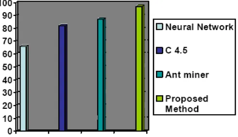
The following graph shows the comparative analysis of our method and various other methods.
VI.CONCLUSION
Pattern recognition has been studied for more than two decades for classification of images and to detect new image in particular class. Still in some cases researcher face difficulty in detecting exact pattern of an image. We have described a comprehensive of methods in a uniform terminology, to define general properties and requirements of local techniques, to enable the readers to select the efficient method that is optimal for the specific application in classification of leaf images. In this paper, a new method for RRG association rule mining is proposed. The “Reverse Rule Generation (RRG)” algorithm is an extraordinary algorithm which generates rule in the reverse manner. Initially the training set is taken as the rule set. Then each rule is decomposed by leaving out each attribute iteratively and inserting the rule in the rule set if the has confidence greater than a pre-specified threshold satisfactory Confidence. Most of the association rule mining algorithm uses support pruning, which results in the pruning of some good quality rule with low support but high confidence. The RRG algorithm doesn’t use support pruning, so it generates all high confidence rules. In fact it can be proved that RRG generates the complete set of high confidence rules
Although by now some progress has been achieved, there are still remaining challenges and directions for future research, such as, developing better preprocessing, enhancement and segmentation techniques; designing better feature extraction, selection and classification algorithms; integration of classifiers to reduce both false positives and false negatives; employing high resolution images and investigating 3D images also. With some rigorous evaluations, and objective and fair comparison could determine the relative merit of competing algorithms and facilitate the development of better and robust systems.
REFERENCES
1. D. A. Clausi, "An analysis of co-occurrence texture statistics as a function of grey level quantization", Can. J. Remote Sensing,28(1), 45-62, 2002.
2. F. Dell' Acqua and P. Gamba. Texture-based characterization of urban environments on satellite sar images. IEEE Transaction on Geoscience and Remote Sensing, 41(1):153-159, January 2003.
3. j. Graham, "Application of the Fourier-Mellin transform to translation-, rotation and scale-invariant plant leaf identification" McGill University, Montreal, July 2000.
4. L. K. Soh and C. Tsatsulis. Texture Analysis of SAR Sea Ice Imagery Using Gray Level Co-Occurrence Matrices. In IEEE Transaction on Geoscience and Remote Sensing, 37(2), (1999).T.Wang and N.Karayaiannis,
5. Jelena Bozek, Mario Mustra, Kresimir Delac, and Mislav Grgic “A Survey of Image Processing Algorithms in Digital mammography”Grgic et al. (Eds.): Rec. Advan. in Mult. Sig. Process. and Commun., SCI 231, pp. 631–657,2009
6. Shuyan Wang, Mingquan Zhou and Guohua Geng, “Application of Fuzzy Cluster analysis for Medical Image Data Mining” Proceedings of the IEEE International Conference on Mechatronics & Automation Niagara Falls, Canada,pp. 36 – 41,July 2005.
7. R.Jensen, Qiang Shen, “Semantics Preserving Dimensionality Reduction: Rough and Fuzzy-Rough Based Approaches”, IEEE Transactions on Knowledge and Data Engineering, pp. 1457-1471, 2004.
8. I.Christiyanni et al ., “Fast detection of masses in computer aided mammography”, IEEE Signal processing Magazine, pp:54- 64,2000 9. Walid Erray, and Hakim Hacid, “A New Cost Sensitive Decision Tree Method Application for Mammograms Classification” IJCSNS
International Journal of Computer Science and Network Security, pp. 130-138, 2006.
10. Ying Liu, Dengsheng Zhang, Guojun Lu, Regionbased “image retrieval with high-level semantics using decision tree learning”, Pattern Recognition, 41, pp. 2554 – 2570, 2008.
11. Kemal Polat , Salih Gu¨nes, “A novel hybrid intelligent method based on C4.5 decision tree classifier and one-against-all approach for multi-class classification problems”, Expert Systems with Applications, Volume 36 Issue 2, pp.1587-1592, March, 2009, doi:10.1016/j.eswa.2007.11.051
12. Etta D. Pisano, Elodia B. Cole Bradley, M. Hemminger, Martin J. Yaffe, Stephen R. Aylward, Andrew D. A. Maidment, R. Eugene Johnston, Mark B. Williams,Loren T. Niklason, Emily F. Conant, Laurie L. Fajardo,Daniel B. Kopans, Marylee E. Brown • Stephen M. Pizer “Image Processing Algorithms for Digital Mammography: A Pictorial Essay” journal of Radio Graphics Volume 20,Number 5,sept.2000 13. Pisano ED, Gatsonis C, Hendrick E et al. “Diagnostic performance of digital versus film mammography for breast-cancer screening”. NEngl J
Med 2005; 353(17):1773-83.
14. Wanga X, Wong BS, Guan TC. ‘Image enhancement for radiography inspection”. International Conference on Experimental Mechanics. 2004: 462-8.
15. D.Brazokovic and M.Nescovic, “Mammogram screening using multisolution based image segmentation”, International journal of pattern recognition and Artificial Intelligence, 7(6): pp.1437-1460, 1993
16. Dougherty J, Kohavi R, Sahami M. “Supervised and unsupervised discretization of continuous features”. In: Proceedings of the 12th international conference on machine learning.San Francisco:Morgan Kaufmann; pp 194–202, 1995.
18. Gianluca Bontempi, Benjamin Haibe-Kains “Feature selection methods for mining bioinformatics data”, http://www.ulb.ac.be/di/mlg
19. M. Tuceryan and A.K. Jain. Texture analysis.In C. H Chen, L. F. Pau, and P. S. P. Wang, editors, Handbook of Pattern Recognition and Computer Vision, chapter 2, pages 235- 276. World Scientific, Singapore, (1993).
20. M. Turk, A. Pentland, "Eigenfaces for Recognition", Journal of CognitiveNeuroscience, 3(1), 71-86 (1991),
21. P. Tzionas, S. E. Papadakis, D. Manolakis, "Plant leaves classification based on morphological features and a fuzzy surface selection technique ",in Fifth International Conference on Technology and Automation,Thessaloniki, Greece, 365-370 (2005).
22. R. M. Haralick, K. Shanmugam, and I.Dinstein. Textural features for image classification. IEEE Transactions on Systems,Man, and Cybernetics, SMC-3(6): 610-621,(1973).
23. S. G. Wu, F. S. Bao, E. Y. Xu, Y. Wang, Y.Chang and Q. Xiang, "A Leaf recognition Algorithm for Plant Classification Using Probabilistic Neural Network" arxiv, 0707,4289v1, [cs.AI], 29 Jul 2007.
24. S. G. Wu, F. S. Bao, E. Y. Xu, Y. Wang, Y.Chang and Q. Xiang, "A Leaf recognition Algorithm for Plant Classification Using Probabilistic Neural Network" arxiv, 0707,4289v1, [cs.AI], 29 Jul 2007.
25. Deepa S. Deshpande “ASSOCIATION RULE MINING BASED ON IMAGE CONTENT” International Journal of Information Technology and Knowledge Management January-June 2011, Volume 4, No. 1, pp. 143-146
26. Holmes, G., Donkin, A., Witten, I.H.: WEKA: a machine learning workbench. In Proceedings Second Australia and New Zealand Conference on Intelligent Information Systems, Brisbane, Australia, pp. 357-361, 1994.
BIOGRAPHY
Aswini Kumar Mohanty is the principal of KMBB college of engineering and technology and a researcher in image mining, data mining and image processing. He has published many research papers in this field and his area of interest is data mining and image processing. Currently he is guiding three M.Tech students and one phd student