Multiportfolio Optimization with CVaR Risk Measure

University of Windsor University of Windsor

Scholarship at UWindsor

Scholarship at UWindsor

Electronic Theses and Dissertations Theses, Dissertations, and Major Papers

2016

Multiportfolio Optimization with CVaR Risk Measure

Multiportfolio Optimization with CVaR Risk Measure

Qiqi Zhang

University of Windsor

Follow this and additional works at: https://scholar.uwindsor.ca/etd

Recommended Citation Recommended Citation

Zhang, Qiqi, "Multiportfolio Optimization with CVaR Risk Measure" (2016). Electronic Theses and Dissertations. 5685.

https://scholar.uwindsor.ca/etd/5685

This online database contains the full-text of PhD dissertations and Masters’ theses of University of Windsor students from 1954 forward. These documents are made available for personal study and research purposes only, in accordance with the Canadian Copyright Act and the Creative Commons license—CC BY-NC-ND (Attribution, Non-Commercial, No Derivative Works). Under this license, works must always be attributed to the copyright holder (original author), cannot be used for any commercial purposes, and may not be altered. Any other use would require the permission of the copyright holder. Students may inquire about withdrawing their dissertation and/or thesis from this database. For additional inquiries, please contact the repository administrator via email

Multiportfolio Optimization with CVaR Risk Measure

by

Qiqi Zhang

A Thesis

Submitted to the Faculty of Graduate Studies

through the Department of Industrial and Manufacturing Systems Engineering in Partial Fulfillment of the Requirements for

the Degree of Master of Applied Science at the University of Windsor

Windsor, Ontario, Canada

2016

Multiportfolio Optimization with CVaR Risk Measure

by

Qiqi Zhang

APPROVED BY:

______________________________________________ Y. Wang

Department of Economics

______________________________________________ F. Baki

Odette School of Business

______________________________________________ G. Zhang, Advisor

Department of Mechanical, Automotive & Materials Engineering

DECLARATION OF ORIGINALITY

I hereby certify that I am the sole author of this thesis and that no part of this thesis

has been published or submitted for publication.

I certify that, to the best of my knowledge, my thesis does not infringe upon anyone’s

copyright nor violate any proprietary rights and that any ideas, techniques, quotations, or any

other material from the work of other people included in my thesis, published or otherwise,

are fully acknowledged in accordance with the standard referencing practices. Furthermore, to

the extent that I have included copyrighted material that surpasses the bounds of fair dealing

within the meaning of the Canada Copyright Act, I certify that I have obtained a written

permission from the copyright owner(s) to include such material(s) in my thesis and have

included copies of such copyright clearances to my appendix.

I declare that this is a true copy of my thesis, including any final revisions, as

approved by my thesis committee and the Graduate Studies office, and that this thesis has not

been submitted for a higher degree to any other University or Institution.

ABSTRACT

The vast majority of studies in portfolio optimization problem are conducted under a single portfolio framework. In the financial industry, the trading of multiple portfolios is usually aggregated and optimized simultaneously. When multiple portfolios are managed together, unique issues such as market impact costs must be dealt with properly.

Conditional Value-at-Risk (CVaR) is a coherent risk measure with the computationally friendly feature of convexity. In this thesis, we propose the novel combination of CVaR with multiportfolio optimization (MPO) problem. To the best of our knowledge, this is the first work to use CVaR to measure risks in MPO problem and investigate the impact of CVaR on MPO problem.

ACKNOWLEDGEMENTS

I would never have been able to finish my thesis without the guidance from my supervisor, committee members, help and support from my friends and family.

I would like to express my deepest and most sincere gratitude to my supervisor, Dr. Guoqing Zhang, for his excellent guidance, his great enthusiasm in the research, his patience in directing my studying, and his kindest support. Whenever I was faced with a problem in research, Dr. Zhang always extends a helping hand. Without Dr. Zhang’s expertise and insight, I would never have been able to finish my thesis. I must also extend my gratitude to Dr. Zhang for the research opportunity he provided for me besides my thesis.

I am grateful for my committee members Dr. Yuntong Wang and Dr. Fazle Baki, for the perceptive suggestions and brilliant ideas they offered me for my thesis. I also would like to thank Dr. Michael Wang for chairing my thesis defense.

TABLE OF CONTENTS

DECLARATION OF ORIGINALITY ... iii

ABSTRACT ... iv

ACKNOWLEDGEMENTS... v

LIST OF TABLES ... viii

LIST OF FIGURES ... ix

Chapter 1 Introduction ... 1

1.1 General Overview ... 1

1.2 Proposed Research ... 3

1.2.1 Research Topic ... 3

1.2.2 Research Methodology and Solution Approach ... 6

1.2.3 Organization of Thesis ... 6

Chapter 2 Literature Review ... 9

2.1 Markowitz’s MVO model ... 9

2.2 Multiportfolio Optimization Problem ... 11

2.3 Risk Measures: VaR and CVaR ... 15

2.3.1 Value-at-Risk ... 15

2.3.2 Conditional Value-at-Risk ... 16

2.4 Transaction Cost in Multiportfolio Optimization Model ... 19

2.5 Fairness in Multiportfolio Optimization Model ... 22

2.6 General Literatures on Portfolio Optimization Models ... 22

Chapter 3 Modelling for MultiPortfolio Optimization Problem ... 28

3.1 Introduction of Multiportfolio Optimization Modelling ... 28

3.1.1 Problem Description ... 28

3.1.2 Notations ... 30

3.1.3 Market Impact Costs and the Pro Rata Scheme ... 34

3.1.4 Utility Functions ... 36

3.2 Modelling ... 38

3.2.1 Model I: Multiportfolio optimization scheme with variance risk measure ... 39

3.2.2 Model II: Multiportfolio optimization scheme with CVaR risk measure ... 44

3.2.3 Model III: Split of market impact cost as decision variables ... 53

3.2.4 Model IV: Adding real life constraints to the multiportfolio optimization Model ... 55

Chapter 4 Solutions and Numerical Results ... 64

4.1 Optimization Software: GAMS ... 64

4.1.1 GAMS Introduction ... 64

4.1.2 GAMS Solvers ... 65

4.1.3 Data Exchange with Excel ... 66

4.2 Data Selection and Preparation ... 67

4.2.1 Scenario Generation ... 67

4.3 Numerical Studies ... 68

4.3.1 Parameters Choices ... 68

4.3.2 Random Number Generation for Initial Holdings ... 70

4.3.3 Numerical Results ... 71

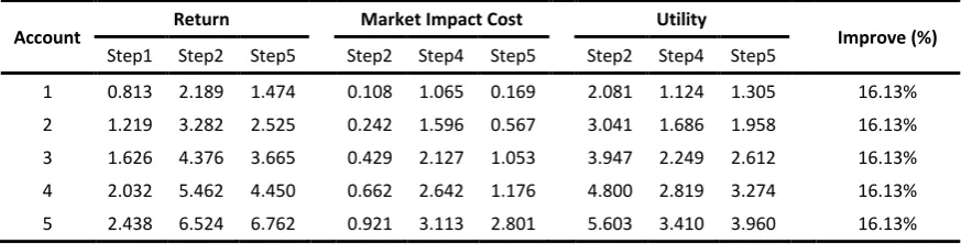
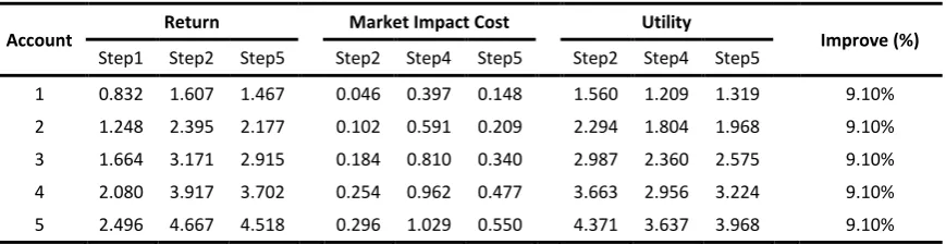
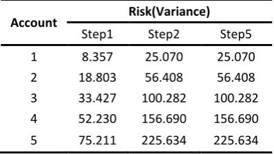
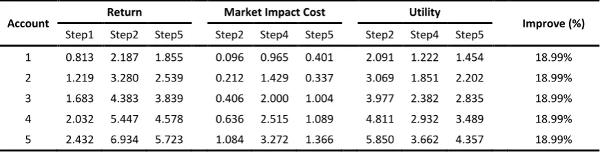
4.3.4 Numerical Analysis ... 82

Chapter 5 Conclusions and Future Work ... 95

5.1 Conclusions ... 95

5.2 Contributions ... 97

5.3 Future Works ... 98

Reference ... 100

LIST OF TABLES

Table 4.1 Symbols and industrial sector of the 20 stocks from NYSE ... 67

Table 4.2 Value of variance for Model I (zero initial holding) ... 72

Table 4.3 Value of return, market impact cost, utility, and improvement rate for Model I (zero

initial holding) ... 73

Table 4.4 Value of CVaR and VaR for Model II (zero initial holding) ... 73

Table 4.5 Value of return, market impact cost, utility, and improvement rate for Model II

(zero initial holding) ... 74

Table 4.6 Value of variance for Model III (zero initial holding) ... 74

Table 4.7 Value of return, market impact cost, utility, and improvement rate for Model III

with Variance risk measure (zero initial holding) ... 74

Table 4.8 Value of CVaR and VaR for Model III with CVaR risk measure (zero initial holding)

... 75

Table 4.9 Value of return, market impact cost, utility, and improvement rate for Model III

with CVaR risk measure (zero initial holding) ... 75

Table 4.10 Value of variance for Model I ... 77

Table 4.11 Value of return, market impact cost, utility, and improvement rate for Model I ... 77

Table 4.12 Value of CVaR and VaR for Model II ... 77

Table 4.13 Value of return, market impact cost, utility, and improvement rate for Model II .. 78

Table 4.14 Value of variance for Model III with Variance risk measure ... 78

Table 4.15 Value of return, market impact cost, utility, and improvement rate for Model III

with Variance risk measure ... 78

Table 4.16 Value of CVaR and VaR for Model III with CVaR risk measure ... 79

Table 4.17 Value of return, market impact cost, utility, and improvement rate for Model III

with CVaR risk measure ... 79

Table 4.18 Value of Variance for Model IV with Variance risk measure ... 80

Table 4.19 Value of return, market impact cost, utility, and improvement rate for Model IV

with Variance risk measure ... 80

Table 4.20Value of CVaR and VaR for Model IV with CVaR risk measure ... 81

Table 4.21Value of return, market impact cost, utility, and improvement rate for Model IV

LIST OF FIGURES

Figure 2.1 Graphical Representation of Maximum Loss, CVaR, and VaR (Uryasev and

Rockafellar, 2000) ... 18

Figure 4.1 Efficient Frontier for five portfolios computed from Model I with variance risk

measure ... 82

Figure 4.2 Efficient Frontier for five portfolios computed from Model II with CVaR risk

measure ... 83

Figure 4.3 Efficient frontier: utility vs variance for five portfolios computed from Model I

with variance risk measure ... 83

Figure 4.4 Efficient frontier: utility vs CVaR for five portfolios computed from Model II with

CVaR risk measure ... 84

Figure 4.5 Improvement rate (%) in different models using different risk measures ... 86

Figure 4.6 Improvement rate of Model II with initial holdings when coefficient  increase

from 1 to 4 ... 87

Figure 4.7 Improvement rate of Model I with initial holdings when coefficient  increase from

1 to 4 ... 87

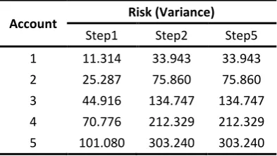
Figure 4.8 Changes of Return and Utility from Step 2 to Step5, taking Model II with initial

holding as example ... 89

Figure 4.9 Comparisons of return and utility in Model I and Model III using Variance risk

measures with initial holdings... 90

Figure 4.10 Comparisons of return and utility in Model II and Model III using Variance risk

measures with initial holdings... 91

Figure 4.11 Returns (4.11a), risks (4.11b) of Model II with random initial holdings for all 5

accounts across scenarios. Historical expected monthly return (4.11c) across scenarios ... 92

Figure 4.12 Portfolio return and utility of Model II with CVaR risk measure when market

impact cost coefficient increase from 0.5 to 2 ... 93

Figure 4.13 Portfolio return and utility of Model III with CVaR risk measure when market

impact cost coefficient increase from 0.5 to 2 ... 93

Figure 4.14 Improvement rate (%) for Model I and Model II when market impact cost

Chapter 1

Introduction

1.1 General Overview

Ever since the breakthrough of Harry Markowitz’s publication on theory of portfolio selection in 1952, the concept of portfolio optimization has been fundamental in the understanding, development and implementation of decision making in the financial industry. Popularly referred to as the Modern Portfolio Theory, Markowitz’s topic of portfolio optimization has received huge attention from both academic and industrial area. Markowitz’s idea of incorporating risk in portfolio investment decisions and applying a disciplined quantitative framework to the management of portfolio investment was novel when it was first introduced. Ever since the introduction of the theory, researchers have been exploring and studying different facets and extensions of portfolio optimization theory for decades. Among which, the problem of multiple portfolio optimization needs further study, given the small amount of existing studies and its closeness to real life financial industry practice.

mathematical optimization. However, it is crucial to mention that while diversification in the portfolio position could help with reducing risk, it could not generally and thoroughly eliminate risk. Through ensuring a diversified portfolio position, risk can be reduced without changing the expected portfolio return [Markowitz, 1952].

Before the introduction of Markowitz’s modern portfolio optimization theory, financial risk was considered as a correcting factor of expected return, and risk-adjusted returns were defined on an ad-hoc basis. At that time, the investment industry’s main focus when making financial decisions was on how to find out and invest in investment assets that have lower price relative to their financial potential, or to put in other way, have high expected returns. Markowitz argued that not only the expected return should be included, it is equally if not more important to take risk from the investment into consideration. In his work, Markowitz used the variance of an asset’s future return as risk measure. Markowitz’s work shows that the riskiness of a single asset is not what is important to the total expected return, but it is its covariance with all other investable assets in the portfolio that really matters. The decisions concerning whether to hold certain assets or not depend on what other assets the investor choose to hold. To acquire the covariance between each assets, however, requires huge amount of data (historical or simulated), which hinder its widespread in practice. Latter models managed to reduce the size of data requirements by eliminating the estimation of correlation between different assets. Furthermore, Markowitz’s traditional model is limited only to the case with elliptical distributions such as normal or t-distributions.

Markowitz’s traditional model and move the research topic closer to the real-world financial industry practice, introducing several new different risk measures which are more computationally attractive, and taking several facets of significant real-world impact in portfolio optimization problems into consideration.

Topics concerning portfolio optimization, such as dealing with the optimization problem of multiple accounts simultaneously or addressing the portfolio optimization problem in a multi-period framework, came into sight and draw attention from both the academia and financial industry in the past decade. After reviewing a great amount of literature and reports, we believe that it is conclusive to say that up till today, after more than 60 years of its introduction, the classical framework of portfolio optimization still needs modification when used in practice, and the topic of portfolio optimization problem still deserves more research efforts into [Kolm and Tütüncü. et al, 2013].

1.2 Proposed Research

1.2.1 Research Topic

(or accounts) are being managed in isolation by the advisors without considering any interrelationship between each account [Iancu and Trichakis, 2014]. However, in practice, those financial advisers in charge with the investment activities of several clients rarely mange a single portfolio (or account) in isolation for the consideration of efficiency in operation. Regardless of the size and scale of such financial institution, they usually serves multiple investment clients, thus multiple investment accounts would be allocated to a single financial adviser. Since one adviser would end up managing more than one investment account, in reality they provide services to multiple accounts simultaneously and act on behalf of multiple portfolios in optimal selection of assets, rebalance, or liquidation of the portfolio. In this thesis, we regard such problem as the multiportfolio optimization problem. The closeness to industry practice alongside with the lack of sufficient existing research focus on multiportfolio optimization problem certainly draws our research interests hence the proposition of this thesis.

do not exist in single portfolio optimization problem. One of the unneglectable differences from the classical model is the transaction cost incurred when pooling multiple trades together, which if not dealt with properly can counteract net investment returns. A small amount of researchers from the academia or the industry realized this need and did research into multiportfolio optimization with transaction cost, trying to capture all the relevant aspects concern with the multiportfolio optimization problem.

1.2.2 Research Methodology and Solution Approach

This thesis uses operations research approaches to formulate and solve the problem. Specifically, linear programming, nonlinear programming, mixed integer linear programming and multi-objective optimization are utilized in the research.

Numerical experiments using real life financial market data are conducted to test the proposed models and the results are analysed in later part of the thesis. Numerical tests with different problem size (number of investment accounts and number of investable assets) is designed and run and its results analysed and verified. The comparisons with existing models are conducted and sensitivity analysis is reported to highlight the impact of different parameters.

The software to be used would include but not limited to the follow: GAMS (General Algebraic Modelling System) and its solvers. MS Excel is used to pre-process the data collected from the real world financial market, and MATLAB is used in numerical analysis of the results from GAMS.

1.2.3 Organization of Thesis

advantage of CVaR over VaR. Last two sections of this Chapter focus on reviewing the studies in market impact costs and different approaches to ensure fairness in multiportfolio optimization.

Chapter 3 is the modelling for the multiportfolio optimization problem we proposed. This chapter discusses in details of the five-step optimization scheme we developed and the model notations and assumptions, the formulation of functions for each accounts and how we allocate the mark impact costs incurred during the optimization to each account. This chapter is highlighted with the model we developed which integrates Conditional Value-at-Risk as risk measure in the constraints. The formulation with variance as risk measure is presented as well for the comparison with the proposed CVaR method in later numerical experiments. In this chapter, a total of four models are developed and they all use the five-step optimization scheme we propose.

Chapter 4 contains the solution approach and preliminary numerical results using real life financial market data from the New York Stock Exchange (NYSE). We provide a brief introduction on the optimization software GAMS and its integrated solvers, followed by a detailed explanation into how the real world stock data from NYSE is chosen and prepared. Discussion on the choices of values of all crucial parameters in all four models, and scenario generation procedure are provided. We run the numerical tests for all four models, perform sensitivity analysis of the results, and conduct comparisons of performances of different risk measures and approaches of splitting the market impact cost.

Chapter 2

Literature Review

Modern Portfolio Theory starts with the seminal work by Harry Markowitz published in 1952. In the paper, Markowitz formulated the mathematical model which has then been regarded as the foundation of modern portfolio model. From an investor’s point of view, the whole purpose of portfolio managing is to gain the highest return possible under a limited amount of capital. To optimally allocate the limited capital between different investable assets seems an easy and solvable problem, however, several factors have to be taken into account, making the portfolio optimization problem more complicated to solve.

2.1 Markowitz’s MVO model

The basic concept and essence of Markowitz’s modern portfolio theory lies in the balance between expected returns and risk. Markowitz presented several types of hypothesis or rule when choosing a portfolio: 1) the investor should strives to maximize the discounted value of expected future returns. 2) The investor should seek maximized expected return while insuring diversification. The rule, to be more specific, requires the investors to invest the funds among diversified securities with highest expected return. 3) The investor should attempt to maximize expected returns at a given risk, or equivalently at a given expected return level try to minimize portfolio risk [Markowitz, 1952].

portfolio with maximum anticipated return may not necessarily be the one with minimum variance. In practice, the investor must consider the trade-off between expected return and variance (E-V); to gain expected return by tolerating the variance, or to give up some expected returns to reduce the risk. However, the E-V rule does agree with any undiversified security which have an extremely higher return and lower risk than all other securities. The E-V rule is the fundament mentioned above for further research studies in the area of finance and portfolio, with a formal name Modern Portfolio Theory (MPT). The model formulated following the E-V rule is based on mean of the return and variance of the return, hence the name Mean-Variance Optimization Model (MVO). In MVO model, risk is associated with the variance (standard deviation) of the distribution of portfolio return, the deviation from the expected return of the portfolio. Out of the set of n investable assets S, assuming the uncertain future return of asset j (j=1,…, n) is rj, and the standard deviation of the

uncertain return is _j, so that the vector of the expected return of all the assets is

T n]

,..., ,

[1 2 

 , where



T n x x x

x[ 1, 2,..., ] represent the proportion of the total funds invested in asset j, and



j j

x 1. Then for a certain

portfolio combination, the variance of total expected return is









j j ij

j j i i j i j j j

jr x E r xx E r E r r E r xx Cov r r x

E x

V ( ) [( ( )) ] [( ( ))( ( ))] ( , )

, 2

And the standard deviation of the future return isp(x) Vp(x)

the Mean-Variance Model: (1) the portfolio variance minimization formulation, subject to target return value R, {minV(x)|s.t:TxR,xX}; (2) the expected return maximization formulations, subject to certain risk constraints,

} , )

( : . |

{maxTx st V x  xX ; and (3) the risk aversion formulation. }

: . | ) (

{maxTxV_p x st xX (𝝀 here is a parameter of risk aversion determined by investors representing trade-off between expected portfolio return and risks. X is the set of all feasible portfolio positions) [F.J.Fabozzi, 2000].

2.2 Multiportfolio Optimization Problem

In practice, financial service providers rarely manage a single portfolio (or account) because they typically offer their services to multiple clients simultaneously. These providers could be from wealth management firms having few individual clients to large investment firms serving a large number of pension, mutual, and insurance funds. An investment manager may need to take charge of multiple portfolios from different clients, with either similar or different sizes or compositions, reflecting potentially different objectives and requirements, levels of risk aversion, etc. [Iancu and Trichakis, 2014].

points out that to provide financial investment management services to large numbers of clients as efficiently as possible relies increasingly on large-scale quantitative portfolio construction methods. Ensuring efficiency in practice usually dictates pooling trades and performing execution of several different investing accounts together.

Goal of multiple portfolio selection problem is fundamentally different from that of the classical single portfolio selection problem. It is a crucial knowing that when being managed simultaneously, investment decisions made for single client affect others’ investment outcomes. As a result, instead of simply optimizing each investment accounts independently, advisors must implement a process different from existing ones that serves to mediate between accounts in decision-making [O’Cinneide et al., 2006].

emphasis on the issue that when making decisions concerning trading, fairness and the common good of all clients must be considered. They formulated an optimization problem that optimizes the portfolios of all clients in an overall sense, which means the objective is to maximize social welfare, i.e., the sum of the objectives functions of individual accounts. The authors argued that through this process fairness for each client ensured, and call this process multi-account optimization (in this thesis we regards multi-account and multiportfolio as the same).

The firm Axioma argues that multiportfolio optimization is the next stage in the progressive evolution of modern investment technologies and platforms, and this technique benefits all parts by making the aggregated trades optimal and fair under given information. Unlike other naïve strategies that sacrifice optimality to achieve fairness, such as randomization and representative accounts, multiportfolio optimization achieves both optimality and fairness during a pooled-trade execution. [Axioma Advisor, 2006]

that accounts are made to participate in artificial game which probably violates the Securities and Exchange Commission rules.

Stubbs and Vandenbussche (2009) did a thorough review on the topics of multiportfolio optimization techniques and properties. They studied the advantages and disadvantages of two economic approaches: the Cournot-Nash equilibrium, and the collusive solution, and presented a unified framework which is able to solve both problems. The focus of this research paper can be justified as fairness between individual investment accounts, for the authors argued that multiportfolio framework can be bias if the issue of fairness is not addressed properly. They also mentioned that definitions of fairness over multiple investment accounts vary among portfolio managers depending on each specific case of investment offering.

Yang et al.(2013) address the multiportfolio optimization problem from a non-cooperative game theory approach; they model the problem as a Nash Equilibrium problem and hence consider a generalized NEP for the case where global constraints are imposed on all accounts, and total welfare is maximized as objective function.

all the portfolios. They proposed a novel, tractable approach by introducing a model addresses all three above mentioned challenges taking general market impact cost into consideration.

2.3 Risk Measures: VaR and CVaR

Ever since the introduction of the classical model, multiple alternative methods of risk management have been studied in the vast majority of literature of modern portfolio theory. The MVO model are only the very basic measures in a portfolio selection. The concept of risk management involves various perspectives, from a mathematical perspective in financial industry, risk management is a procedure for shaping a loss distribution (such as an investor’s risk profile). Though widely studied, among a great deal of innovations in the risk measurements, only a few have been accepted and adapted in real life financial daily operations by practitioners. Beside the implementation of variance or standard deviation as the measurement of risks, other well-known and widely used measure of risk including Value-at-risk and Conditional Value-at-risk also draw attention as practical methods of risk management in portfolio optimization problem.

2.3.1 Value-at-Risk

Value-at-Risk works on a given investment time horizon and confidence level α. Given a specified confidence level α (commonly set at 0.90, 0.95, and 0.99), the VaRa

Definition 1 (Value-at-Risk). With a given confidence level α, VaR_(L)is a lower α-percentile of the random variableL:

} ) ( | min{ )

( 

 L  l F l 

VaR _x

If loss is a normally distributed random variableL~N(,2), then VaR is proportional to the standard deviation [Sarykalin, Serraino and Uryasev, 2008]:

  



(L)FL1( )  fL1( )

VaR

However, the easiness and intuitiveness in the formulation of VaR is counterbalanced by unfavourable mathematical properties; a lack of both convexity and continuity as a result of being a function of the confidence level α bring numerical difficulties into the problem. It will be discussed and analysed in later part of this paper.

2.3.2 Conditional Value-at-Risk

Conditional-Value-at-Risk (CVaR) was introduced as a new approach to reduce the risk of high losses during portfolio optimization, its other names includes mean excess loss, mean shortfall, or tail VaR. As defined above, given a probability α as confidence level, VaRa is the threshold value of loss of a portfolio, so that the loss

will not exceed this value with a probability α. The CVaR_ is the conditional expectation of losses above the threshold value of loss. CVaR is, by definition, always no less than the VaRa. Consider a random loss function f(x,y) associated

also possible. The vector y represents uncertainties such as uncertain returns, or market variables that can affect the loss, with a probability density functionp(y).

Definition 2 (Conditional-Value-at-Risk): With p(y) given, the CVaR_ can be denoted by



However, an analytical expression p(y) for the implementation of the approach is not needed. It is sufficient to have an algorithm (code) which generates random samples fromp(y). A two-step procedure can be used to derive analytical expression for p(y) or construct a Monte Carlo simulation code for drawing samples from p(y) [Rockafellar and Uryasev, 2000].

Rockafellar and Uryasev proposed an alternative approach for CVaR calculation, it is a minimization formula that works as a replacement forCVaR . Define a function



F( , ) (1 ) 1 [ ( , ) ] ( )

Such that

) , ( minF x l CVaR

l 

  _

Function F(x,l) has a favourable mathematical feature, as a function of loss, )

, (x l

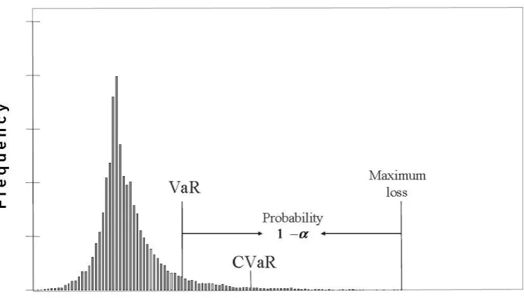
Figure 2.1 Graphical Representation of Maximum Loss, CVaR, and VaR (Uryasev and Rockafellar, 2000)

According to the definition of CVaR and VaR, Figure 2.1 shows a graphical representation of the relationship between the value of CVaR, VaR and maximum loss.

Rockafellar and Uryasev (2000) argues that CVaR is a superior risk measure to

VaR in optimization applications in many ways. When returns of the portfolio R is discretely distributed, VaR is nonconvex and discontinuous with respect to portfolio positionsxT, these properties makes the VaR hard to optimize computationally. VaR

continuous function with respect to confidence level α, and a convex function of portfolio positions vector T

x .

CVaR measures outcomes that hurt the most, which gives itself a clear engineering interpretation. It can be reduced to convex programming, in some cases, to linear programming (i.e., for discrete distributions). This attractive feature can greatly reduce the computational complexity in optimization problem [Sarykalin, Serraino and Uryasev, 2008].

From the point of regulatory requirements, advantages of CVaR are recognized by financial supervision committees. Basel Committee (2012) propose in the Basel III regulations to move the quantitative risk metrics system from VaR to Expected Shortfall (also known as CVaR or tail-VaR).

The conclusion, on the different usage of VaR and CVaR in different situation, is that CVaR is preferable with an accurately constructed model for tail loss, while VaR

is a better choice when an acceptable good model for tail loss is not available. But it is still important not to ignore the properties of VaR that bring difficulties into optimization.

2.4 Transaction Cost in Multiportfolio Optimization Model

accounted for in existing literatures of multiportfolio optimization problem. Market impact is the effect a trader has on the market price of an asset when it sells or buys the asset. It is the extent to which the price moves up or down in response to the trader’s activities. For example, the selling of a large number of shares of a particular stock may drive down the stock’s market price [Fabozzi et al. 2010].

An important component of the objective function of modern portfolio rebalancing techniques that rely on optimization is the trading costs. As a result of the buying or selling activities which may drive the asset’s market price down or up, the actual price of a certain asset usually differs from the expectation (usually worse than expected price) [Savelsbergh et al. 2010].

Under the multiportfolio optimization settings, the transactions costs incurred by each portfolio heavily depend on the trading activity of other portfolios. That is to say that the transaction costs for a given account may depend on not only the account’s own trading requirements but also the overall level of trading. In a multiple portfolio setting, transaction costs typically increase for each account when trading of the accounts are pooled [O’Cinneide et al., 2006].

One of the primary type of transaction costs is the market impact costs, it is where the core of the difference between single and multiportfolio selection problem lies. These market impact cost originate from price impact and limited “at-the-money” liquidity [Iancu and Trichakis, 2014].

particular asset, which is called the pro rata scheme. Even though this scheme is easily understandable and applicable and sometimes regarded as fair [Fabozzi et al. 2007], it works only under the assumption that the market impact costs are separable across assets, and it also fails to properly reflect all interactions between the accounts which leads to unfairness. In literature, the issue of splitting market impact costs is seldom discussed, the market impact cost is either not considered or split in the pro rata fashion [Iancu and Trichakis, 2014].

Assume w0_j is the initial portfolio holding of an account on behalf of asset j,

then w_jis the optimal portfolio holdings of this account. There are many different

models for the transaction cost t.

1) The simplest one is the linear transaction costs, which is under the assumption that the costs are proportional to the trading size. Given a certain

percentagec_j, the transaction cost function could be formulated as:





n

j

j i

jw w

c 1

0

.

2) To take a step further from the linear model, a piecewise-linear transaction model is more realistic, especially for large trades. The costs increase alongside with the increase in the trading size. Here we do not include the formulation because piecewise-linear transaction cost is not the main focus of this thesis.

3) A more general formulation of the transaction cost is to assume that the

transaction cost takes form:  _i 0_j

j

jw w

t



2.5 Fairness in Multiportfolio Optimization Model

In multiportfolio optimization, a central problem associated with the optimal solution is the fairness issue. Because the trading decision for one account affect the outcomes for other accounts, the advisor must take into consideration fairness and the common good of all clients [O’Cinneide et al., 2006]. Iancu and Trichakis (2014) points out that when one of the accounts is much larger in size than the others, smaller accounts can suffer from a shortage of liquidity. For those small accounts, the socially optimal solution is not fair in the sense that they can achieve a better return profile by acting alone. If the separate accounts belong to individual clients who care about their own utilities only, those “smaller” clients may not be satisfied with the socially optimal solution.

It is understandable that the primary goal of optimization process is to strive for optimality, but under the multiportfolio setting, it is more than just necessary to obtain fairness in the allocation of trades across portfolios [Iancu and Trichakis, 2014]. Consider a simple example in which all accounts are optimized in isolation which means no sharing of information across the investors, if fairness is not ensured, then investment returns of the accounts can probably be very disproportionate [Savelsbergh et al. 2010]. Accounts that obtain less gains than that under the independent optimization setting would rightfully refuse to share information and participate in multiportfolio optimization.

2.6 General Literatures on Portfolio Optimization Models

chapter we introduce the general review of literature conducted while searching for desirable research topic.

Fang and Lai (2006) considered liquidity to treat the uncertain expected return and risk as fuzzy numbers and proposed a linear programming model for portfolio rebalancing with transaction costs. Furthermore, based on fuzzy decision theory, a portfolio rebalancing model with transaction costs is proposed.

Tanaka and Gotoh (2010) studied and implemented the constant rebalancing strategy for multi-period portfolio optimization via CVaR under nonlinear transaction costs. They quoted that to solve a multi-period portfolio optimization with a constant rebalancing strategy problem is considerably easy for log-optimal portfolio. But when a risk measure is taken into consideration in the model, the problem becomes nonconvex, plus if the size of the question is large, then even the state-of-the art NLP solvers would have difficulties finding local optimal solution. Furthermore, if transaction costs are introduced, these costs cannot be easily dealt with because transaction costs would prevent the problem from having a compact representation. The authors developed a local search algorithm for solving the constant rebalanced portfolio optimization problem under nonlinear transaction costs. In this algorithm, linear approximation problems and nonlinear equations are iteratively solved via a linear programming (LP) solver and Newton’s method, respectively.

to reach. To deal with the difficulty, the author then proposed two suboptimal policies based on the optimal policy for unconstrained cases.

Wang and Li (2014) considered V-shaped transaction cost in rebalancing model with self-finance strategy, meaning that the investor will not supply any additional investment amount.. They pointed out the main contribution of the paper to be the introduction of a new constraint that confirms the rebalancing necessity of the existing portfolio needs to be adjusted. CVaR as risk measure is used in the objective function to be minimized.

Yu and Lee (2009) considered several criteria including risk, return, short selling, skewness, and kurtosis. They studied a total of five portfolio rebalancing models to determine the important design criteria for portfolio model. They implemented a fuzzy multi-objective programming approach to found out that the rebalancing models that consider transaction cost, including short selling cost, are more flexible and their results can reflect real transactions. For future study, they suggested that rather than a portfolio selection based on historical return, a portfolio selection that is able to predict future return can be developed in order to meet this fast-changing environment.

Fabian (2008) proposed decomposition frameworks to solve two-stage stochastic portfolio optimization models with CVaR in the objectives function or as constraints. The two-stage decomposition framework has the decision/observation/decision/observation pattern.

multi-period portfolio optimization model with CVaR as risk measure to be minimized in the objective function. Moreover, proportional transaction costs and market imperfections are also considered in the model. The authors also mentioned that their genetic algorithm can solve the stochastic optimization model with transaction cost and large simulated paths very efficiently, while existing papers reported that large dimension of the stochastic model results in difficulty in computation and only a small number of simulated paths being considered for the brevity of computation.

Meng and Jiang (2010) presented a time-consistent dynamic risk measure: the sum of CVaR of each period in the multi-period model. A Markov decision process model is used in getting the optimality equation. The model and the result was then applied in a multi-period portfolio optimization problem with the CVaR in the objective functions to be minimized.

Najafi and Mushakhian (2015) characterized their multi-period portfolio selection model with three parameters: the expected value, semivariance and CVaR at a given confidence level α. The authors’ hybrid Genetic Algorithm (GA) and particle swarm optimization (PSO) algorithm to solve the multi-period model. Taguchi experimental design method is applied to ensure the parameters of the model are wisely chosen for the sake of the performance of the hybrid GA-PSO meta-heuristic algorithm.

players (stock certificates) with different risk abilities, the obtained return was distributed in accordance with the weight of each player in the portfolio using Shapley Vector.

Yang and Rubio (2013) considered the case of multiportfolio optimization, in which in practice individual investment accounts are usually pooled together for execution, so the aggregated effects such as market impact must be treated carefully. Multiportfolio optimization aims at finding optimal rebalancing between different investing accounts. The paper implemented non-cooperative game theory and presented a Nash Equilibrium problem.

Wu and Chen (2015) consider a multi-period MV portfolio optimization under a dynamic risk aversion assumption (regime switching). According to the authors, in the real world, it is quite usual that the decision-making process in different portfolio selection period is conducted by different decision-makers (players), hence they treat the problem as a non-cooperative game and proposed that the decision-maker n can only choose the control the portfolio position strategy πn to maximize objective

function given that the successors choose the equilibrium strategy. The authors derived the subgame perfect Nash equilibrium strategy and equilibrium value function in closed-form.

In brief conclusion, both stochastic programming of multi-period model and

Chapter 3

Modelling for MultiPortfolio Optimization Problem

As discussed in Chapter 2, the uniqueness of multiportfolio optimization problem compared with the classical single portfolio optimization problem inevitably render both the academy and industry in search for mathematical models that can accurately and efficiently address the differences. To address the problem of multiportfolio optimization, based on existing literature we introduce our MPO models with Conditional Value-at-Risk (CVaR) as risk measures. And we also focus on the allocation of trading incurred market-impact costs. Compared with researches done in the past on the MPO problem, we mainly focus on two topics, namely, the measurement of risks and the allocation of costs between portfolios. Among the existing literatures on the MPO problem, the question of how risk is measured has never been given enough emphasis on. The introduction of the risk measure of CVaR

in our model distinguishes our method from the existing researches. In terms of splitting the market impact costs, we implement both the industrial standard approach of splitting the market impact cost in a pro rata fashion, and the solution method by Iancu and Trichaskis (2014) to treat market impact cost as decision variables.

In this chapter, we present the formulation of our multiportfolio optimization problem with CVaR as risk measure. The formulation with variance as risk measure will also be constructed.

3.1 Introduction of Multiportfolio Optimization Modelling

3.1.1 Problem Description

accounts simultaneously. Thus, the problem of optimizing the portfolio selections of n

accounts simultaneously from an investment pool consists of m assets is regarded as the Multiportfolio Optimization Problem. Note that one account represents one client served by the financial advisor. The trading activities of an account act on behalf of the client’s portfolio investment preferences and target, while properties such as total available investment funds represents the client’s monetary input. The three terms account, client, and portfolio are used interchangeably in our problem. The investment pool consists of a total number of m risky assets. As introduced above, when one financial advisor manages multiple accounts, all trading activities of the n accounts are pooled together in a whole by the advisor during the optimization process.

To be more specific on the executions of trading of the assets under the multiportfolio framework proposed above, the term “pooling trades” indicates that the portfolio advisor combines all buying orders of a certain asset by all participating portfolios into one order, and submits the aggregated trades to the market at once, the same with all selling orders of a certain asset by all portfolios as well.

thesis consider both the implicit and explicit part of the transaction costs. For the implicit market impact cost, we use two different approaches to split the costs across the accounts, namely the pro rata approach and the decision variable approach. The explicit part of the transaction costs is modelled as linear transaction cost proportional to the trading size.

To address the MPO problem, we designed four different optimization models, each with different decision variables or risk measures, for the above mentioned problem. The five steps optimization schemes are designed to perform from the advisor’s point of view and to help the advisor in the portfolio selection decision making process by providing the optimal portfolio position for each account participating in the multiportfolio optimization. Notations and assumptions used in the schemes are introduced and discussed in details in the following section of this chapter.

3.1.2 Notations

In this section we introduce indices, parameters, variables, and expressions that are used in the later part of the thesis.

Model Indices, Parameters and Variables:

Indices

i - Index for portfolio (or accounts),

i



I



{

1

,...,

n

}

j - Index for assets, jJ {1,...,m};

Model Parameters：

i

C - Total available capital for the ith account;

i

w - The vector to denote the initial holding of the ith _account, m

i

w , i.e.,

ij

w denotes the initial holding in the jth asset on behalf of the ith

account;

) (s j

y - The rate of return of the jth asset on the sth scenario;

 - The vector of expected return,m

, i.e., _j denotes the expected

return of the jth asset. _j is the mean of ys_j across all scenarios;

 - The covariance matrix of the return of the assets,







i

 - The risk preference coefficients for each account (client’s risk tolerance),

1



i

 ,_in ;

i

 - The minimum risk level for the ith account, this value is a result from the

first optimization step in our optimization scheme.

j

 - Market impact cost coefficients for the jth asset. Calibrated from data,

satisfying _j 0

 - Constant for transaction cost model,





1

i

x - The vector to denote the portfolio position (in units of currency) of the ith

account. Let mn

n 

(x1,x2,...,x )

x be the matrix containing portfolio position for all accounts. m

i

x , i.e., x_ij denotes the portfolio position in the jth asset on behalf of the ith account;

Auxiliary Variables:



ij

x - The buy order of the ith account on the jth asset, where





max _{ij ij}

ij x w

x   ;



ij

x - The sell order of the ith account on the jth asset, where









max _{ij ij}

ij x w

x    ;



i

x - The buy order vector of the ith _account;



i

x - The sell order vector of the ith _account;



ij

x and x_ijare positive variables.

Functions:

) , ( i i

t x x - The market impact costs resulting from the execution of tradesxi;

) ( _i

i

u x - The utility derived by the ith account; the functions {ui(xi)}iI are

required to be concave and expressed in units of currency for all accounts;

i

) ,..., (U1 Un

f - The welfare functionf :n . This function is assumed to be component wise increasing;

The expressions for the functions above are given in later part of this section.

Assumptions:

a. The problem is considered under a stylized, single-period rebalancing framework;

b. In this problem, the financial adviser provide portfolio selection, rebalancing or liquidation services to n distinct portfolio accounts;

c. There exist a same pool of m risky assets that are investable for all the accounts. The available pool of assets could be the entire universe of stocks in the Standard & Poor 500, or New York Stock Exchange;

d. All trading in this single-period framework is assumed to be not frictionless for all accounts, i.e., the transaction costs incurred during monetary transactions of all n portfolios are nonzero. This assumption is relaxed in Model IV;

e. There exist both explicit (linear transaction costs) and implicit (market impact cost) part of transaction costs in the models. Only the market impact costs is considered in the first three models, and both market impact costs and linear transaction costs are considered in the last model;

f. To follow the common practice in the financial industry, during one rebalancing period, the financial adviser pool all the buy and sell orders from all n accounts together into a single buy and single sell order, respectively; g. Possibility of cross-trading, where the financial advisor net buy and sell orders

say, any trades on behalf of all the accounts must be operated through the market, no in-house trading is allowed in our model;

h. The market impact costs is separable across assets, i.e., the buying and selling of a particular asset does not affect the market impact costs incurred during the buying and selling of the other assets. The expression of this assumption will be provided below;

i. In our models, the market impact cost is split across the accounts after the optimization problem is solved. We employ two means of splitting the cost, to split it in pro rata scheme, or as decision variables set by the solver.

j. The portfolio selection problem under a single-portfolio setting is formulated as maximizing the net utility Ui, which is represented by the portfolio return

less market impact cost. Under a multiportfolio setting, the net utility Ui is then

jointly optimized by solving a multi-objective optimization problem;

k. Even if the financial adviser makes rebalancing decisions and places buying and selling orders for each portfolio separately, the transaction costs incurred by each portfolio would still depend on the activity of other portfolio. To put it in the form of the market impact cost,  >1;

l. Shorting selling of any asset by any account is prohibited in the thesis.

3.1.3 Market Impact Costs and the Pro Rata Scheme

Let the market impact costs due to the execution of tradesxijand  ij x be        









j x x x x

t

As described in assumption (h), the total market impact cost is separable across assets, the expression for this assumption is as follow

(











i x t x x

x

t

The pro rata scheme

The most common approach of splitting market impact costs incurred during pool trading of multiportfolio optimization is the pro rata approach, which indicates that each account is charged a cost proportional to its share of the total trade for a particular asset. In a pro rata fashion, for market impact costs that are separable across the assets, the trades for the jth asset are{x_ij}_i_I, the ith account is charged a cost of







 a J

aj J a aj j I a aj ij x x t x x ) ,

( ,



i



I

,

j



J

Which brings the total market impact cost charged to a particular portfolio i is expressed as follow



_





j a J

aj J a aj j I a aj ij

i t x x

x x

3.1.4 Utility Functions

To express the total utility generated from the rebalancing trades for the ith

account, the expected utility isui(xi). The most widely-used expression to quantify the utility is in units of currency, as follow

i T i i

u (x ) x , iI

And if the risk is considered, the risk-adjusted expected utility function is as follow,

Risk

u T _{i i}

i

i(x) x   , iI

Note that the risk measure in the above expression can be replaced by CVaR, variance, which will be introduced as a major part of the model.

The net expected utility Ui for the i

th _{account, is the total expected return ( )}

i i x u

for the ith account deducted the amount charged from that account as market impact costs.



i

U u_i(x_i)-t_i, iI

3.1.5 Risk Measure

Conditional Value-at-Risk (CVaR) as risk measure

Known that the return on a portfolio is the sum of return made through individual assets invested in the portfolio beingTx, the loss of the portfolio is then the negative of the return, taking the form

x x

f( ,_s)T

Introducing a function 





F [ ( , ) ]

) 1 ( 1 ) , (     

 , function

) , (   x

F is piecewise linear with respect to



Rockafellar and Uryasev (2000) proved the following theorems;

THEOREM 1 As a function of



differentiable. The CVaRa of the loss associated with xX can be determined from

the formula

) , ( min _ 



 F x

CVaR 

THEOREM 2 Minimizing the CVaR_a of the loss associated with x over all xX is

equivalent to minimizing F(x,) over all

(

x

,



)



X



R

) , ( min min ,  

 F x

CVaR

x

x 

The minimization of F_(x,) over all

(

x

,



)



X



R

necessarily unique, such that

x



 _{gives the corresponding}

a

when f(x,s)is convex w.r.t x, in which case, if the constraints are such that X is a

convex set, the joint minimization is an instance of convex programming.

To make the function of CVaRa more optimization-solver friendly, we

introduce auxiliary variables y1,...,ysfor all S scenarios. Andy  x T

s

s ( ) , ys 0,

for all s.

The introduction of function F(x,) makes the calculation of CVaRaeasier

for optimization software. For the formulation of our model, we apply this approach to calculate CVaRa.

The Variance as risk measure

Variance of the portfolio is formulated as follow;

x

x







where is the covariance matrix calculated from data.

3.2 Modelling

The execution of dividing the market impact costs incurred during multiportfolio optimization practice and charge the costs to each individual portfolio according to certain rules is also a major focus of this section. Market impact costs in our models, due to its categorization as the implicit type of transaction costs, is estimated using a nonlinear, quadratic function which takes the trading of the assets as arguments. To split the costs, we implement two different approaches, namely the pro rata approach and the decision variable approach.

3.2.1 Model I: Multiportfolio optimization scheme with variance risk measure

The following part of this section discusses the modelling of the above mentioned 5-step scheme with the notations and assumptions introduced in Section 3.1. We start simple and explain our 5-step optimization scheme with the classical risk measure variance. Model I takes variance as risk measure, and the market impact cost is split in a pro rata fashion across accounts. Detailed explanations of the objective functions and constraints for all five steps are provided below.

Step1. Solve the following portfolio optimization problem for each account i

independently with variance as objective function to be minimized.

i T i x

x 

min (1)

s.t xiXi (2)

In this step, we solve the variance minimization problem subject to a set of feasible trade constraint Xi in order to obtain the minimum value of the

Let{x_iopt}_iIdenote the optimal solution obtained. Then the optimal value of

the objective function is_i xopt_i Tx_iopt.

Step2. Solve the following independent optimization problem for each account i,

with net utility as objective function to be maximized subject to constraint for

upper bound for variance.

max{ui(xi)t(xi,xi)} (3)

s.t x_iTx_i _i_i (4)

xiXi (5)

where ui(xi)is the expected portfolio return, and ( , )  

i i

t x x is the market impact cost.

In this step, we still consider the standard single account setting and maximize the expected portfolio net utility, subject to a constraint of the variance of the expected portfolio return.

A more detailed formulation of this step is as below,

max{ [( ) ( ) ]}

1

 



  



 



j j i

T

x x

x (6)

s.t x_iX_i (7) x_iTx_i _i_i (8) x_i, x_i 0 (9)

step. This step is to solve a maximization problem of the expected return of the

ith account with a constraint to limit variance of the portfolio return relative to a benchmarkii. The value ofi, wherei 1, is set by either the client or by

the financial advisor.

Note: The optimal solution IND i

x differs from the optimal solution opt i

x

Step3. Aggregate optimal buy and sell orders for each asset from Step 2 across

all n accounts



i IND i

x ,



i IND i )

(x (10)

Step 2 solves the individual net utility maximization problem for all n accounts, and as a result acquires the solution of n optimal solution of vectorx_i . However, the single portfolio optimization model of Step 2 overlooks the presence of other accounts participating in the investment markets, buying and selling the assets. The ignorance of the existence of other accounts can cause significant underestimation of the true market impact costs incurred by the trading activity of every account. To take into account the effects of aggregated trading of all accounts managed by the advisor, the buy and sell orders of each asset j are aggregated to calculate the total market impact cost. For the jth asset, the aggregated buy and sell orders from all accounts are



( and



( , respectively. The resulting market impact cost for

the jth _{asset is then formulated as}

} ) ) ( ( ) ) ( {( ) ) ( , ) ( ( 1 1 1 1   









 _{ } n

i IND ij n i IND ij n i j IND ij n i IND ij

j x x x x