Evolutionary Algorithms for Multiobjective Optimization with Applications in Portfolio Optimization

(1)

ABSTRACT

RADHAKRISHNAN, ALAMELU. Evolutionary Algorithms for Multiobjective Optimization with Applications in Portfolio Optimization. (Under the supervision of Dr. Negash Medhin.)

Multiobjective optimization (MO) is the problem of maximizing/minimizing a set of non-linear objective functions (modeling several performance criteria) subject to a set of nonnon-linear constraints (modeling availability of resources). The MO problem has several applications in science, engineering, finance, etc. It is normally not possible to find an optimal solution in MO, since the various objective functions in the problem are usually in conflict with each other. Therefore, the objective in MO is to find the Pareto front of efficient solutions that provide a tradeoff between the various objectives.

Classical techniques assign weights to the various objectives in the MO problem, and solve the resulting single objective problem using standard algorithms for nonlinear optimization. Moreover, these techniques only compute a single solution to the problem forcing the decision maker to miss out on other desirable solutions in the MO problem.

(2)

EVOLUTIONARY ALGORITHMS FOR MULTIOBJECTIVE

OPTIMIZATION WITH APPLICATIONS IN PORTFOLIO

OPTIMIZATION

by

ALAMELU RADHAKRISHNAN

A thesis submitted to the Graduate Faculty of North Carolina State University

in partial fulfillment of the requirements for the Degree of

Master of Science

OPERATIONS RESEARCH

Raleigh, North Carolina

March 27, 2007

APPROVED BY

Dr. Jeffrey Scroggs Dr. Salah Elmaghraby

(3)

BIOGRAPHY

(4)

ACKNOWLEDGEMENTS

(5)

List of Tables

2.1 Total Returns for four assets between 1960 and 2003 (Cornuejols and Tütüncü

[4]). . . 21

2.2 Rates of Return for the four assets. . . 22

2.3 Geometric mean for the four assets. . . 23

2.4 Covariance between the four assets. . . 23

(7)

List of Figures

1.1 A plot of 200 Pareto optimal solutions in the decision variable space (top) and objective function space (bottom) for (1.7). . . 8 1.2 A plot of 200 Pareto optimal solutions in the decision variable space (top) and

objective function space (bottom) for (1.8). . . 9

(8)

Chapter 1

Multiobjective Optimization

1.1 Introduction

Optimization is the process of finding solutions that minimize or maximize a set of objective functions subject to constraints. When multiple objectives are present, the optimization prob-lem is called amultiobjective optimization(MO) problem. Multiobjective optimization (Ehrgott [6]), Miettinen [17], Deb [5], Coello Coello et al. [2]) is also referred to as multi-criteria opti-mization, multi-performance or vector optimization (Jahn [10]).

An MO problem can be formally defined as finding (Osyczka [20]) a vector of decision variables that satisfies constraints and optimizes a vector function whose elements represent the objective functions.

The objective functions form a mathematical description of performance criteria which are usually in conflict with each other. Hence, the term optimize means finding a solution which would give the values of all the objective functions acceptable to the decision maker.

(9)

best solutions by the decision maker.

One of the first applications of multiobjective optimization was in economics to solve public investment problems in the 1960s (Cohon and Marks [3]). Other applications arise in control (Zadeh [30]), and water resource planning (Marglin [15]). Multiobjective optimization is also frequently used in engineering, science, industry and finance (Coello Coello et al. [2] and Deb [5]).

This chapter is organized as follows: Section 1.2 provides a mathematical definition of a multiobjective optimization problem. Section 1.3 provides an application of multiobjective optimization in solving the portfolio selection problem in finance. Section 1.4 discusses an important concept in multiobjective optimization called Pareto optimality. Section 1.5 briefly describes different methods including classical methods and evolutionary algorithms for solving multiobjective optimization problems. Finally, Section 1.6 describes our contribution in the thesis.

1.2 Mathematical formulation of a multiobjective optimization

problem

Consider the problem

min f(x)

such that gj(x) ≤ 0, j = 1, . . . , m hl(x) = 0, l= 1, . . . , p.

(1.1)

The vector x ∈ IRn _{contains the decision variables in (1.1). The set} _S ₌ _{_x _∈ _IRn _| _g j(x) ≤

0, j = 1, . . . m, hl(x) = 0, l = 1, . . . p} is the feasible region of (1.1) and depicts constraints

such as the limited availability of resources in the problem. The mappingf :IRn_→_IRk_defined

by f(x) = (f1(x), . . . , fk(x))T contains the k objective functions (possibly nonlinear) of (1.1).

We define thefeasible objective regionZ as the image of the feasible regionSunder the mapping

f, i.e., Z = {y ∈ IRk _| _y

i = fi(x), i = 1, . . . , k,∀ x ∈ S}. We assume that all the objective

(10)

equivalent to minimizing the function −fi(x).

It is important to distinguish between the constraint space S and the objective function space Z in multiobjective optimization. The set Z plays an important role in the concept of Pareto optimality in multiobjective optimization, and we discuss this in Section 1.4.

1.3 Example: The portfolio selection problem in finance

Consider the classic portfolio selection problem in finance where our aim is to find an optimal portfolio of securities (stocks, bonds, etc.) that provides a tradeoff between the expected return and the risk involved. An investor wishes to invest certain amount of money in n securities,

S1, . . . , Sn. Each securitySi has a random return whose expected value and standard deviation

are given by µi and σi respectively. Moreover, the correlation coefficient of the returns of

two securities Si and Sj is denoted by ρij. Given this information, the n×n symmetric

positive semidefinitecovariance matrix is given by Σ = (σij), whereσii=σi2,i= 1, . . . , n and σij =ρijσiσj,∀ i6=j. If xi denotes the proportion of the total money invested in securitySi,

the expected returnE[x], and the variance Var[x] of the resulting portfoliox= (x1, . . . , xn) are

given by

E[x] =µ1x1+. . .+µnxn=µTx, (1.2)

and

Var[x] =

n

X

i,j=1

ρijσiσjxixj =xTΣx. (1.3)

The set of feasible portfolios is given byX={x∈IRn_: _Ax₌_{b, Cx}_≥_d_}_{. The set}_X _includes

the following constraints:

n

X

i=1

xi = 1 indicating that the available capital is invested in the n

securities, andxi ≥0 depicting short sales restrictions (where the investor cannot sell securities

that he/she does not own). Other constraints inXinclude diversification (that imposes a limit on the amount alloted to a particular security or the securities of a sector) and transaction costs (Cornuejols and Tütüncü [4]).

(11)

variance (risk). Such a portfolio is called an efficient portfolio. An efficient portfolio is also defined as a portfolio that has minimum variance among all portfolios that guarantee a certain value of expected return or the one that has the maximum return over all portfolios whose variances are less than a prespecified value. The set of all the efficient portfolios form a curve in 2D space (standard deviation vs expected return), also known as the efficient frontier.

The portfolio selection problem is also known in the literature as Markowitz’s portfolio optimization problem (Markowitz [16]) or the mean-variance optimization (MVO) problem. The efficient frontier can be calculated in three different ways (Cornuejols and Tütüncü [4]):

1. Minimize the variance: In this scheme, one produces the set of efficient portfolios by solving a quadratic programming (QP) model given by

min 1 2x

T_Σ_x

s.t. µT_x _≥ _R

Ax = b

Cx ≥ d

(1.4)

for values of R ranging between Rmin and Rmax. The first constraint in (1.4) indicates

that the expected return should at least meet the target value R. The QPs are convex and can be solved efficiently using interior point methods (Cornuejols and Tütüncü [4]). 2. Maximize the return: In this scheme, one produces the set of efficient portfolios by

solving a quadratically constrained model given by

max µT_x

s.t. 1 2x

T_Σ_x _≤ _σ2

Ax = b

Cx ≥ d

(1.5)

for values of σ2

ranging between σ2

min and σ

2

max. The first constraint in (1.5) indicates

that the variance (risk) should be less than the target value σ2

(12)

once again be solved using conic programming and interior point methods (Cornuejols and Tütüncü [4]).

3. Minimize the variance and maximize the return simultaneously: In the thesis, we will solve the portfolio optimization as the following multiobjective optimization problem

min   

1 2x

T_Σ_x

−µT_x

  

s.t. Ax = b

Cx ≥ d.

(1.6)

The two objectives in (1.6) minimize the risk and to maximize the return over the set of feasible portfolios. Maximizing µT_x _{is equivalent to minimizing} ₋_µT_x_{. Intuitively, it}

is clear that the expected return and the risk are conflicting objectives, since one has to take a large risk to produce a large return. The set of efficient (Pareto) solutions to the multiobjective optimization problem (1.6) form the efficient portfolio. We will discuss our numerical results in solving a portfolio selection problem in Section 2.4.

1.4 Pareto Optimality

(13)

Definition 1 A decision vector x∗

∈ S is Pareto optimal if there is no other decision vector

x∈S such that fi(x)≤fi(x∗) for alli= 1, . . . , k and fj(x)< fj(x∗) for at least one index j.

Pareto optimality can also be defined in terms of the objective function space Z as below: Definition 2 An objective vector z∗

∈Z is Pareto optimal if there is no other objective vector

z ∈ Z such that zi ≤ zi∗ for all i= 1, . . . , k and zj < zj∗ for at least one index j, i.e., z∗ is

Pareto optimal if the decision vector corresponding to it is Pareto optimal.

The above concept of Pareto optimality is sometimes referred to as global Pareto optimality or strongly efficient solutions. The other related concepts are locally Pareto optimal, and weakly Pareto optimal solutions. They can be defined as follows:

∈ S is weakly Pareto optimal if there is no other decision vector x∈S such thatfi(x)< fi(x∗) for all i= 1, . . . , k.

∈S is locally Pareto optimal if there exists δ >0 such that

x∗

is Pareto optimal inS∩B(x∗

, δ) where B(x∗

, δ) is a suitable neighborhood ofx∗

of radiusδ.

Local Pareto optimality and weak Pareto optimality can also be defined in terms of the objective function space (Miettinen [17]).

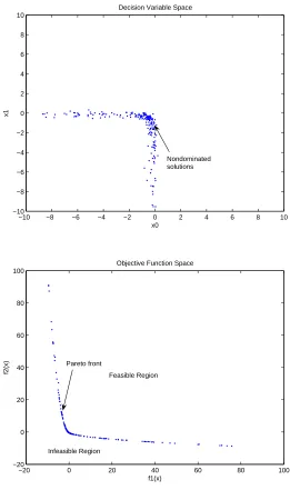
The Pareto optimal solutions or the strongly efficient solutions form a hypersurface known as thePareto frontin the objective function space Z. These solutions represent tradeoffs from which the decision maker picks the desired solution. The Pareto optimal solutions are also referred to as non-dominated solutions since it is not possible to improve an objective without worsening at least another objective. Consider the following multiobjective problem

min   

x2 0+x1

x0+x21

  

s.t. −10≤x0 ≤10

−10≤x1≤10.

(14)

Figure 1.1 shows the plot of 200 Pareto optimal solutions in the decision variable space (top) and objective function space (bottom) for the multiobjective optimization problem (1.7). As seen in Figure 1.1 (bottom), the Pareto optimal solutions form a Pareto front in the objective function space. The Pareto front divides the feasible and non optimal solutions from the infeasible solutions. The Pareto optimal solutions in Figure 1.1 form a front in the decision variable space. The formation of a front in the decision variable space depends on the mapping

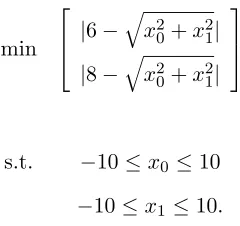
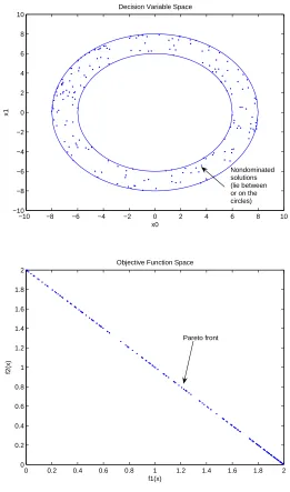
f between the Pareto optimal solutions in the objective function space and the decision variable space. Consider another multiobjective problem

min   

|6−qx2 0+x

2 1|

|8−qx2 0+x

2 1|

  

s.t. −10≤x0 ≤10

−10≤x1≤10.

(1.8)

(15)

Figure 1.1: A plot of 200 Pareto optimal solutions in the decision variable space (top) and objective function space (bottom) for (1.7).

−10 −8 −6 −4 −2 0 2 4 6 8 10

x0

x1

Decision Variable Space

Nondominated solutions

−20 0 20 40 60 80 100

f1(x)

f2(x)

Objective Function Space

Feasible Region

(16)

Figure 1.2: A plot of 200 Pareto optimal solutions in the decision variable space (top) and objective function space (bottom) for (1.8).

−10 −8 −6 −4 −2 0 2 4 6 8 10

x0

x1

Decision Variable Space

Nondominated solutions (lie between or on the circles)

0 0.2 0.4 0.6 0.8 1 1.2 1.4 1.6 1.8 2

f1(x)

f2(x)

Objective Function Space

(17)

1.5 Methods to solve multiobjective optimization problems

The methods that are used to solve multiobjective optimization problems can be broadly clas-sified as

1. Classical Methods

2. Evolutionary Algorithms.

1.5.1 Classical Methods

In classical methods, the various objective functions of the multiobjective optimization problem are combined together in a single objective function

ˆ

f(x) =

k

X

i=1

wifi(x), (1.9)

wherewi >0 are appropriate weights. The single objective function ˆf(x) is minimized over the

feasible setSusing traditional nonlinear optimization techniques for a single objective function. Classical methods are also classified as a priori or progressive techniques based on when the weights are assigned to the objective functions as follows:

1. A priori: In this method, the weights are assigned to the objective functions before optimization is performed. One of the requirements of this method is that the order of importance of the objectives has to be known ahead of time. Once the weights are chosen, they are fixed throughout the optimization procedure. Setting the weights before optimization omits desirable solutions from the model. For the assigned weights to be effective, the objective functions need to be normalized to factor in their different dynamic ranges. This is not an easy task because it requires the knowledge of the extreme values of the objective functions. These drawbacks make a priori preference methods (Miettinen [17]) very difficult to use.

(18)

method is better than the a priori technique because corrections are made using the information obtained during optimization. However, prior knowledge of the problem is often required to define a scheme of preference to bias the search so that the decision maker’s biases do not lead to undesirable solutions.

To summarize, one of the main shortcomings of classical methods is that some prior knowledge of the problem is required to assign reasonable weights. In classical methods, it is not possible to find multiple solutions in a single run and also not possible to find all the Pareto optimal solutions. This causes the decision maker to miss out other desirable solutions to a problem. However, these algorithms are known to converge to a Pareto optimal solution of the multiob-jective problem (Stewart [29]). For more details on classical methods, we refer the reader to Deb [5], Coello Coello et al. [2], and Miettinen [17].

1.5.2 Evolutionary Algorithms

The classical methods are extensively being replaced by evolutionary algorithms, that are based on Darwin’s theory of evolution. Evolutionary algorithms include evolutionary strategies (Rechenberg [27] and Schwefel [28]), genetic algorithms (Holland [9] and Goldberg [8]), and differential evolution (Price and Storn [24], [25]).

All evolutionary algorithms aim to improve the existing solution using the techniques of recombination, mutation, andselection. The general paradigm is as follows:

1. Initialization: The initial population consisting of µ members (parents) is chosen ran-domly.

2. Recombination: The µparent vectors randomly recombine with each other to produce

λ≥µ child vectors.

3. Mutation: After recombination, the λchild vectors undergo mutation where a random deviation is added to each child vector.

(19)

parent vectors to become parents in the next generation, whereas in (µ, µ+λ) strategy, the best µ vectors from the child and parent populations become parents in the next generation.

5. Termination: The number of iterations (generations) performed depends on the conver-gence criterion chosen.

We briefly mention a few advantages of evolutionary algorithms over classical methods. 1. Evolutionary algorithms are multiobjective optimization techniques that generate a set

of equally desirable solutions using the concept of Pareto optimality. The decision maker chooses a solution from the set of available Pareto solutions, and thus implicitly assigns a set of weights. Unlike classical methods, no weights are assigned to the various objectives during the course of the algorithm. Therefore, the solutions are found without introducing bias.

2. In evolutionary algorithms, we deal with a population of desirable solutions in each itera-tion whereas in classical methods we deal with only one soluitera-tion. Unlike classical methods where a pre-defined rule is used to search through the solutions, evolutionary algorithms use probabilistic rules to search through solutions. Moreover, evolutionary algorithms are easier to implement and are typically faster than classical techniques. Moreover, several parallel implementations are currently available (Lampinen [13]).

(20)

1.6 Contribution of the thesis

We investigate the use of differential evolution (an evolutionary algorithm) to solve multiob-jective optimization problems in this thesis. Unlike classical methods, differential evolution directly solves the multiobjective problem to find the Pareto front of efficient solutions. More-over, this algorithm uses probabilistic rules to search for solutions and is very efficient in solving medium sized multiobjective optimization problems. We use differential evolution to compute theefficient frontierin the classical Markowitz mean-variance optimization problem in finance and illustrate our results on an example.

(21)

Chapter 2

Differential Evolution: An

Evolutionary Algorithm for

Multiobjective Optimization

2.1 Introduction

In this thesis, multiobjective optimization problems are solved using an evolutionary algorithm called differential evolution. The idea of differential evolution was first conceived by Kenneth Price and Rainer Storn (Price and Storn [24], [25]) in 1995. Differential evolution is an evolu-tionary algorithm that uses the techniques of recombination, mutation and crossover to improve solutions. It is further categorized as an evolutionary strategy because it encodes real valued parameters as floating point numbers.

(22)

existing randomly selected population vectors. Differential evolution is self-adjusting because the perturbations that the difference between the vectors are large in the beginning of the opti-mization and become smaller as the algorithm approaches the optimal solution. This property makes differential evolution computationally less expensive and less complicated than the other evolutionary strategies.

2.2 Algorithm for Differential Evolution

Consider the multiobjective problem

min f(x)

s.t. gj(x) ≤ 0, j = 1, . . . , m xi ≤ ui, i= 1, . . . , n xi ≥ li, i= 1, . . . , n

(2.1)

wherex∈IRn_and_f₍_x_{) = (}_f

1(x), . . . , fk(x))T. We assume that any equality constrainth(x) = 0

in the original MO problem is written as two inequality constraints h(x) ≤0 and −h(x) ≤ 0 and thus represented in the constraint set of 2.1.

A quick review of notation: Letr,N pdenote the generation and the size of the population in each generation respectively. The population in therth generation is denoted byPr_∈_IRn×N p_.

Let xr

j,i denote the jth component of the ith population vector in the rth generation. We

present the differential evolution algorithm that solves the multiobjective optimization problem below:

Algorithm 1 (Differential Evolution for Multiobjective Optimization)

1. Initialize: Set generation count r = 1. Let Pr _{be the initial population matrix, whose}

entries xr

j,i are computed as

xr

(23)

where K is a random number chosen uniformly from [0,1]. 2. Mutation: Generate mutated vectors

vr

i = xrr0+F(xrr1−xrr2), i= 1, . . . , N p, (2.3)

where for each i, r0, r1, and r2 are three distinct indices (different from i) randomly chosen from {1, . . . , N p} and F > 0 is a suitable parameter whose value is generally chosen to be less than 1.

3. Crossover: Generate N p trial vectors, where the ith vector is given by

ur_j,i=     

vr

j,i : if K ≤Cr or j=j ′

xr

j,i : otherwise.

(2.4)

where K is a random number chosen uniformly from [0,1], Cr (crossover probability) is a parameter in[0,1], and j′

(24)

4. Selection:

xr_i+1 =                                                                                ur i if                                                                       

∀j∈ {1, . . . m} gj(uir), gj(xri)≤0

and

∀l∈ {1, . . . k} fl(uri)≤fl(xri)

or

∀ j∈ {1, . . . m} gj(uri)≤0

and

∃ j∈ {1, . . . m} gj(xri)>0

or

∃ j∈ {1, . . . m} gj(uri)>0

and ∀ j∈ {1, . . . m} g′

j(uri)≤g ′ j(xri) xr

i otherwise

(2.5)

where g′

j(uri) = max (gj(uri),0) andg ′

j(xri) = max (gj(xri),0) are the constraint violations.

5. Update generation count: Set r =r+ 1. Ifr > rmax, STOP. Else, return to Step 2.

2.3 Features of differential evolution

We briefly mention the salient features of this algorithm.

1. The mutation performed is calleddifferential mutationdue to the use of the scaled differ-ence of two randomly chosen population vectors. The parameterF is a scaling parameter that controls the rate at which the population evolves.

(25)

mutated vector over the current population vector. During crossover, to ensure that the trial vector is not identical to the current vector, the value of parameter at thej =j′

th position is taken from the mutated vector.

4. The restriction onr0, r1, and r2 guarantees that differential evolution’s unique strategy of mutation and crossover does not reduce to simply mutation, crossover or arithmetic recombination.

5. The parameters F and Cr control the convergence speed and the robustness of the al-gorithm. By trial and error, suitable values for the parameters have been found to be

N p = 5×n . . .30×n, F = 0.90, and Cr = 0.9. Depending on the problem, the values

can be modified to increase the rate of convergence. For details on how to choose values, we refer the reader to Price, Storn and Lampinen [26] and Price and Storn [24], [25]. 6. Since trial vectors are generated through a series of steps, it is necessary to check whether

they satisfy the boundary conditions. The computationally less expensive as well as the commonly used rule is

ur_j,i =     

K.(uj−lj) +lj : if urj,i < lj orurj,i > uj ur

j,i : otherwise

(2.6)

where, j= 1, ...., n,i= 1, . . . , N pandK is a uniform random number between 0 and 1. 7. The feature that makes differential evolution unique is the shape of the probability

(26)

8. The control parameters F and Cr also influence the working of the algorithm. The parameter F reduces the occurrence of stagnation (especially in smaller populations) by preventing the trial vectors from being very close to each other. The parameter Cr also helps prevent stagnation by introducing vectors in addition to the existing N p(N p−1) vectors to choose from. These additional vectors are created during crossover by skillfully combining parameters from the trial as well as target vectors. Due to the dependence of the distribution on the above mentioned factors, it is practically impossible to predict the shape of the PDF (Lampinen and Storn [19]).

9. In the differential evolution algorithm, the inequality constraints and the objective func-tions are handled during selection. The selection technique is based on Lampinen’s direct constraint handling method (Lampinen [11], [12]) that is used to solve constrained single objective problems. It employs Pareto dominance to check the feasibility of a trial vector and also to decide whether the trial vector is a non dominated solution. The trial vector replaces the current population vector in the next generation when one of the following three conditions is met:

(a) The trial and current vectors are both feasible and the objective function values of the trial vector are smaller than that for the current vector.

(b) The trial vector is feasible but the current vector is infeasible.

(c) The trial vector is infeasible but the constraint violation of the trial vector is less than the current vector.

The objective function values are compared only if the trial vector and the current population vector are both feasible implying that the selection scheme directs the search first towards the feasible regions before considering the objective values.

2.4 Computational Results

(27)

whose future expected returns are estimated using data collected from previous years. Table 2.1 shows the total returns for the four assets for 44 years between 1960 and 2003. The S & P 500 Index, the 10-year Treasury Bond Index, the 1-day federal fund rate and the NASDAQ Composite Index are used to compute the returns on Assets 1,2,3 and 4 respectively.

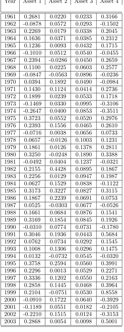
LetT Rit,i= 1, . . . ,4 andt= 0, . . . , T denote the total return of assetiin the yeartwhere t= 0 is 1960 and t=T is 2003. We compute the rate of returns

rit =

T Ri,t−T Ri,t−1

T Ri,t−1

i= 1, . . . ,4, t= 1, . . . , T (2.7)

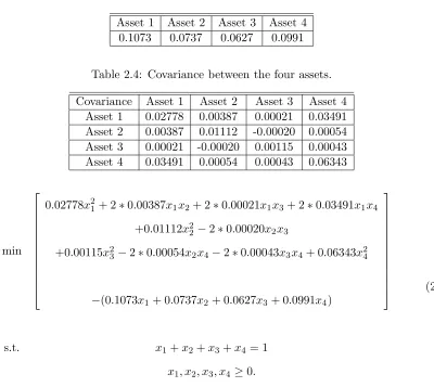
using the entries in Table 2.1 and the entries are displayed in Table 2.2. We then compute the expected value and the variance for the portfolio selection problem 1.6 in Section 1.3 as follows: The geometric mean (and not the arithmetic mean) is used in the computation of the expected value to account for the multiplicative nature of the rate of return over time. The geometric mean for asseti is calculated as

µi = (

T

Y

t=1

(1 +rit)) 1

T −1 (2.8)

and the results are displayed in Table 2.3. The covariance between the assetsiandjis calculated using the formula

Σi,j =

1

T T

X

t=1

(rit−ˆri)(rjt−rˆj) (2.9)

where ˆri and ˆrj are the arithmetic mean of assets i and j. The covariance matrix is given in

(28)

Table 2.1: Total Returns for four assets between 1960 and 2003 (Cornuejols and Tütüncü [4]).

(29)

Table 2.2: Rates of Return for the four assets.

Year Asset 1 Asset 2 Asset 3 Asset 4

(30)

Table 2.3: Geometric mean for the four assets.

Asset 1 Asset 2 Asset 3 Asset 4 0.1073 0.0737 0.0627 0.0991

Table 2.4: Covariance between the four assets. Covariance Asset 1 Asset 2 Asset 3 Asset 4

Asset 1 0.02778 0.00387 0.00021 0.03491 Asset 2 0.00387 0.01112 -0.00020 0.00054 Asset 3 0.00021 -0.00020 0.00115 0.00043 Asset 4 0.03491 0.00054 0.00043 0.06343

min              

0.02778x21+ 2∗0.00387x1x2+ 2∗0.00021x1x3+ 2∗0.03491x1x4

+0.01112x2

2 −2∗0.00020x2x3

+0.00115x2

3 −2∗0.00054x2x4−2∗0.00043x3x4+ 0.06343x24

−(0.1073x1+ 0.0737x2+ 0.0627x3 + 0.0991x4)

             

s.t. x1+x2+x3+x4= 1

x1, x2, x3, x4 ≥0.

(2.10)

The multiobjective problem (2.10) is solved using the differential evolution algorithm. We implemented the algorithm in MATLAB. In order to check that the MATLAB code is correct, we used a three-asset portfolio problem (Cornuejols and Tütüncü [4]) with a known efficient frontier. We compared the efficient frontier obtained using the multiobjective approach with the known efficient frontier and found them to be the same. The values of the control parameters for (2.10) were chosen as F = 0.95, Cr= 0.9 and N p= 200. The algorithm is run forrmax = 500

iterations. Initially, we ran the algorithm for rmax = 1000 iterations. Since, there was no

difference between the results for 1000 and 500 iterations, we set rmax = 500. The equality

constraintx1+x2+x3+x4= 1 is handled as two inequality constraints. The code took about

(31)

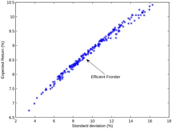
efficient portfolios that provide a tradeoff between the expected return and the risk involved. Table 2.5 lists the efficient portfolios for a set of expected returns and variances. We plot the Pareto front objective function space in Figure 2.1. The front represents the efficient frontier for the portfolio selection problem.

Figure 2.1: Efficient Frontier: standard deviations versus rate of returns for (2.10).

2 4 6 8 10 12 14 16 18

6.5 7 7.5 8 8.5 9 9.5 10 10.5

Standard deviation (%)

Expected Return (%) Efficient Frontier

One advantage of using multiobjective optimization model for portfolio selection is that the efficient portfolios for different rates of return are found by solving (2.10) only once whereas in the models (1.4) and (1.6), the problem has to be solved once for each value of R and σ2

(32)

Table 2.5: Efficient Portfolios of the four assets for different rates of return. Rate of Return Variance Asset 1 Asset 2 Asset 3 Asset 4

0.0711 0.0017 0.1246 0.2245 0.6403 0.0106 0.0755 0.0030 0.2353 0.0837 0.6435 0.0375 0.08 0.0049 0.2750 0.2903 0.3840 0.0508 0.0851 0.0071 0.4548 0.1732 0.3654 0.0066 0.0901 0.0108 0.5194 0.2380 0.1995 0.0431 0.0947 0.0159 0.6494 0.0143 0.2569 0.0794 0.1004 0.0200 0.8003 0.0999 0.0753 0.0245

because it resembles the Pareto front.

2.5 Conclusions and Future work

The thesis is concerned with multiobjective optimization problems where one minimizes a set of nonlinear objective functions over a feasible set described by nonlinear constraints. The aim in multiobjective optimization is to find the Pareto front of efficient solutions that provide a suitable tradeoff between the various objectives in the problem.

We use an evolutionary algorithm called differential evolution to solve multiobjective op-timization problems in the thesis. This algorithm has the following advantages over classical methods for multiobjective optimization: Differential evolution solves the multiobjective opti-mization problem directly and computes the Pareto front of optimal solutions. On the other hand, classical methods assign a priori weights to the various objectives in the multiobjective problem and solve the resulting single objective problem using classical algorithms for nonlin-ear optimization. As a result, the differential evolution algorithm finds a population of Pareto optimal solutions (rather than a single biased solution that depends on the weights) for a mul-tiobjective problem. Moreover, the differential evolution algorithm is very easy to implement and is usually faster than classical methods on small-medium sized multiobjective problems.

(33)

portfolio selection problem.

(34)

Bibliography

[1] C.W. Carrol,The created response surface technique for optimizing non linear restrained systems, Operations Research, 9, 1962, pp. 169-184.

[2] C.A. Coello Coello, D.A. Van Veldhuizen, G.B. Lamont,Evolutionary Algorithms for Solving Multiobjective Problems, Kluwer Academic Publishers, 2002.

[3] J.L. Cohon and D.H. Marks,A Review and Evaluation of Multiobjective Programming, Water Resources Research, 11(2), 1975, pp. 208-220.

[4] G. Cornuejols and R. Tütüncü,Optimization Methods in Finance, Cambridge Uni-versity Press, 2007.

[5] K. Deb, Multiobjective Optimization using Evolutionary Algorithms, John Wiley & Sons Ltd., 2001.

[6] M. Ehrgott,Multicriteria optimization, Springer - Berlin, New York, 2000.

[7] K.R. Frisch, The logarithmic potential method of convex programming, Memorandum, University Institute of Economics, Oslo, 1955.

[8] D.E. Goldberg, Genetic Algorithms in search optimization and machine learning, Addison-Wesley, 1989.

(35)

[10] J. Jahn, Vector Optimization: Theory, Applications, and Extensions, Springer Verlag, 2004.

[11] J. Lampinen,A Constraint Handling Approach for the Differential Evolution Algorithm, Proceedings of the 2002 Congress on Evolutionary Computation, Volume 2, pp. 1468-1473, 2002.

[12] J. Lampinen, Multi-Constrained Non-Linear Optimization by the Differential Evolution Algorithm, edited by R. Roy , M. Koppen, S. Ovaska, T. Furuhashi and F. Hoffman, Soft Computing and Industry - Recent Advances, pp. 305-318, Springer Verlag, 2002.

[13] J. Lampinen, Differential Evolution - new naturally parallel approach for engineering design optimization, edited by B.H.V. Topping, Development in computational mechanics with high performance computing, Civil-Comp Press, Edinburgh, 1999, pp. 187-197. [14] J. Lampinen and I. Zelinka, Mixed Variable Non-Linear Optimization by Differential

Evolution, Proceedings ofNostradamus’99, 2nd International Prediction Conference, 1999. [15] S. Marglin,Public Investment Criteria, MIT Press, Cambridge, Massachusetts, 1967. [16] H. Markowitz,Portfolio Selection, Journal of Finance, 7, 1952, pp. 71-91.

[17] K. M. Miettinen,Nonlinear Multiobjective Optimization, Kluwer Academic Publishers, 1999.

[18] J.A. Nelder and R.Mead, A simplex method for function minimization, Computer Journal, 7, 1965, pp. 308-313.

[19] J. Lampinen and R. Storn, New Optimization Techniques in Engineering, edited by G.C. Onwubolu and B.V. Babu, Springer Verlag, 2004.

(36)

[21] V. Pareto,Cours d’Economie Politique, Libraire Droz, Geneve, 1964 (the first edition in 1896).

[22] V. Pareto,Manual of Political Economy, The Macmillan Press Limited, 1971 (the orig-inal edition in French in 1927).

[23] W.L. Price, A controlled random search procedure for global optimization, edited by L.C.W. Dixon and G.P. Szeg¨o, Toward global optimization 2, North Holland, Amsterdam, 1978, pp. 71-84.

[24] K.V. Price, R.M. Storn,Differential Evolution - a simple and efficient adaptive scheme for global optimization over continuous spaces, Technical Report TR-95-012, ICSI, 1995. [25] K.V. Price, R.M. Storn, Differential Evolution - a Simple and Efficient Heuristic for

Global Optimization over Continuous Spaces, Journal of Global Optimization,11 (4), 1997, pp. 341-359.

[26] K.V. Price, R.M. Storn, J.A. Lampinen,Differential Evolution: A Practical Approach to Global Optimization, Springer, 2005.

[27] I. Rechenberg,Evoltutionsstrategie, Frommann-Holzboog, Stuttgart,1973. [28] H.P. Schwefel,Evolution and optimum seeking, Wiley, 1994.

[29] T.J. Stewart,Convergence and Validation of Interactive Methods in MCDM: Simulation Studies, edited by M.H. Karwan, J. Spronk and J. Wallenius, Essays in Decision Making: A Volume in Honor of Stanley Zionts, Springer-Verlag, 1997, pp. 7-18.