Kim, Yuntae. Evaluation of Frequentist and Bayesian Inferences by Relevant Simu-lation. (Under the direction of Professor Peter Bloomfield.)
Statistical inference procedures in real situations often assume not only the basic assumptions on which the justification of the inference is based, but also some addi-tional assumptions which could affect the justification of the inference. In many cases, the inference procedure is too complicated to be evaluated analytically. Simulation-based evaluation for such an inference could be an alternative, but generally tion results would be valid only under specific simulated circumstances. For simula-tion in the parametric model set-up, the simulasimula-tion result may depend on the chosen parameter value.
In this study, we suggest an evaluation methodology relying on an observation-based simulation for frequentist and Bayesian inferences on parametric models. We describe our methodology with the suggestions for three aspects: factors to be mea-sured for the evaluation, measurement of the factors, and evaluation of the inference based on the factors measured. Additionally, we provide an adjustment method for inferences found to be invalid.
The suggested methodology can be applied to any inference procedure, no matter how complicated as long as it can be codified for repetition on the computer. Un-like general simulation in the parametric model, the suggested methodology provides results which do not depend on specific parameter values.
validity of the inferences under his classical strategy since it ignores the uncertainty in the choice of a subset model.
BY RELEVANT SIMULATION by
YUNTAE KIM
A dissertation submitted in partial satisfaction of the requirements for the degree of
Doctor of Philosophy
in
STATISTICS in the
GRADUATE SCHOOL at
NC STATE UNIVERSITY 2000
Peter Bloomfield ,Chair Montserrat Fuentes
Biography
Acknowledgements
Contents
List of Tables vii
1 Introduction 1
1.1 Overview . . . 1
1.2 Literature review . . . 5
I
General framework
11
2 Set-up 12 3 Ideal sampling properties 16 4 Methodology 20 4.1 Measurement . . . 204.1.1 Relevant distribution for parameter . . . 22
4.1.2 Monte Carlo approximation . . . 23
4.2 Evaluation . . . 24
4.3 Adjustment . . . 26
II
Application
27
5 Particulate matter-mortality regression 28 5.1 Background . . . 285.2 Linear model analysis . . . 30
5.3 Piecewise linear model analysis . . . 38
5.4 Inference results . . . 41
6 Evaluation of inferences 46 6.1 Simulation scheme . . . 46
6.3 Adjustment of inferences . . . 55
III
Conclusion
57
List of Tables
5.1 Frequentist inferences for PM coarse linear effect . . . 41
5.2 Empirical Bayesian inferences for PM coarse linear effect . . . 42
5.3 Frequentist inferences for PM fine linear effect . . . 43
5.4 Empirical Bayesian inferences for PM fine linear effect . . . 43
5.5 Frequentist inferences for PM coarse threshold effect . . . 44
5.6 Frequentist inferences for PM fine threshold effect . . . 45
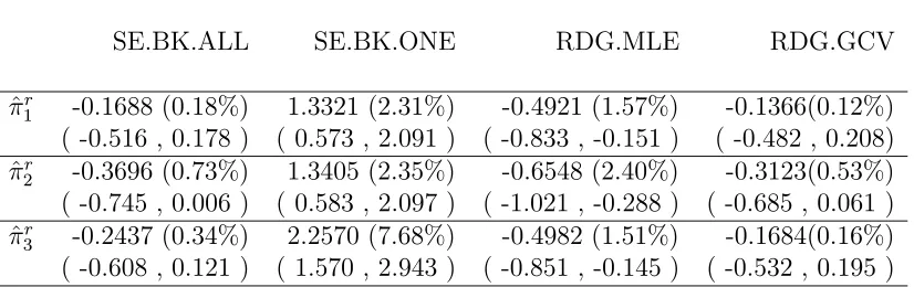
6.1 Relevant estimates and 95% confidence intervals for coverage probabil-ity of the interval estimators in the PM coarse linear model . . . 49
6.2 Relevant estimates and 95% confidence intervals for expected length of the interval estimators in the PM coarse linear model . . . 49
6.3 P-value of Kolmogorov-Smirnov test for uniformity of the repeated pv.rr(X) in the restricted relevant space by rr = 1 in the PM coarse linear model . . . 50
6.4 Relevant estimates and 95% confidence intervals for expected p-value and posterior probability under alternative in the PM coarse linear model 50 6.5 Relevant estimates and 95% confidence intervals for a performance measure of the Bayesian hypothesis test in the PM coarse linear model 51 6.6 Relevant estimates and 95% confidence intervals for MSE of point es-timators in the PM coarse linear model . . . 52
6.7 Relevant estimates and 95% confidence intervals for bias of point esti-mators in the PM coarse linear model . . . 52
6.8 P-value of Kolmogorov-Smirnov test for uniformity of the repeated pv.β1(X) in the restricted relevant space by rr = 1 in the PM fine threshold model . . . 53
6.9 Relevant estimates and 95% confidence intervals for coverage probabil-ity of the interval estimators in the restricted relevant space byrr = 1 in the PM fine threshold model . . . 53
Chapter 1
Introduction
1.1
Overview
A reasonable statistical inference procedure would be justified by some validity and performance proved under some basic assumptions. But in many real situa-tions for statistical procedures, the validity and performance are affected by further assumptions and decisions inevitably involved in the procedures. Here are some ex-amples:
• The classical strategy in the regression model having a suite of highly correlated covariates is to select a subset model, and then make the inference assuming the subset model. We call this kind of method a selection and estimation (S/E) procedure. All the justification of the inferences coming from the subset model can not be guaranteed since it ignores the uncertainty in the selected subset model;
• Inferences based on asymptotic theory could be justified only for infinitely many samples, but the real situation always involves finite samples;
• The performance of ridge estimators depends critically on the choice of the ridge constant; there is as yet no concensus as to an optimal choice; and
• More generally, the repeated sampling properties of Bayesian procedures depend on the choice of the prior distribution; data-dependent priors for pseudo-Bayes methods have been proposed for certain problems, but no general theory exists.
When we get an inference result from such statistical procedures, we may want to check whether or not the additional assumptions and decisions distort validity and performance of the inference. However, the situation can be too complicated to get an analytical evaluation for the inference in many cases. For example, the complicated selection step in the S/E procedure for regression modeling, makes it impossible to get an analytical evaluation tool. Simulation study could be an alternative way of evaluating such a complicated inference procedure, but the evaluations coming from general simulation study would only apply to the specific simulated circumstances. For the simulation in the parametric model, the simulation result may depend on the chosen parameter value.
We suggest an evaluation methodology relying on an observation-based simulation for general frequentist and Bayesian inferences on parametric model. The suggested methodology can be applied to any inference procedure, no matter how complicated, as long as it can be codified for repetition on the computer. Unlike general simulation, the suggested methodology provides the evaluation result which does not depend on the parameter value.
Generally speaking, evaluation of an object has three main components:
• Which “factor” of the object is interesting for evaluation?
• How does one “measure” the factor?
• How does one “evaluate” the object based on the measurement for the factor?
Our suggestion for the factors of interest are the ideal sampling properties of the inference. For examples, a valid confidence interval guarantees the coverage proba-bility of including true parameter in the sampling space is larger than the nominal value. The justification for the p-value of the frequentist test of a simple null hypoth-esis is that repeated samplings of p-value under the null follow uniform distribution over (0,1). We will adopt this frequentist criterion for both frequentist and Bayesian inferences. It seems natural to expect the frequentist inferences to have the ideal sampling properties. Though Bayesian inference procedures are not designed for ideal sampling properties, it is also expected to satisfy them well in order to be a reasonable statistical framework. (See examples of Bayesian inference having a good frequentist property in Section 1.2.)
All the interesting ideal sampling properties of inferences could be expressed as the conditions for parameter dependent frequentist risks over a portion of parameter space. For example, achievement of the nominal coverage probability of a ν-level confidence interval ciν(X) for some interesting function φ(θ) of the parameter with parameter space Θ can be expressed as
same idea with RSM in Section 1.2.)
The simulation-based RSM could provide not only an estimate for the risk, but also a measure of precision, such as standard error. Using these quantities, formal inference procedures like confidence intervals and hypothesis tests could be provided to determine whether the risk condition is satisfied.
Additionally, we provide the adjustment methods for the inferences founded to be invalid with respect to an ideal sampling property by the suggested evaluation scheme. Details of the methods for fixing up invalid p-values and interval estimators to have their ideal sampling properties are provided. We will call the presented evaluation methodology for general inference “evaluation scheme using RSM”.
The justification of the stronger standards for particulate matter (PM) introduced by the U.S. Environmental Protection Agency (EPA) in 1997 has been argued by the industrial and other groups. They claim that the new standards are lack of scientific verification. This argument has been led to some statistical analyses for the effect of PM on mortality. Smith, Kim, Fuentes & Spitzner (2000) is a recent study for the comparison of the short-term effects of fine PM (particulate matter of aerody-namic diameter 2.5 µm or less) and coarse PM (particulate matter of aerodynamic diameter between 2.5 µm and 10 µm) on mortality of elderly based on a new data source from Phoenix, Arizona over a time period from 1995 to early 1998. They re-ported the significant effects for both size particles through some regression analyses of daily average of elderly mortality on daily average of PM concentration and some confounding variables; linear effect for PM coarse and nonlinear threshold effect for PM fine with the threshold value around 20–25 µg/m3 were found to be significant.
As to the threshold effect of PM fine, they found highly significant effect above the threshold value, but insignificant effect below the threshold.
and also reach a conclusion about the short-term effects of PM coarse and PM fine on mortality. Even though the conclusions based on only three-year data of a single city can not be considered conclusive, we could avoid concerns about invalidity of the inferences through the methods presented here.
In the rest of this chapter, some related literature will be reviewed. The gen-eral framework of “evaluation scheme using RSM” for inference will be described in detail in Chapters 2–4, and the application of the presented methodology to the PM-mortality regression model will be explained in Chapters 5–6.
1.2
Literature review
Simulation, relevant simulation and bootstrap
In general simulation under a parametric model f(x | θ), the data points are simulated using a two-step procedure: first a value for the parameter θis chosen, and then observations are generated from f(x|θ). The simulation results over a portion of the parameter space would be examined, and some conclusion would be extracted. However, simulation results often focus on a relevant region of the parameter space to the researchers judgment or interests. For example, Viallefont, Raftery & Richardson (1998) provided a simulation-based comparison of the classical variable selection strategy and BMA (Bayesian modeling average) procedure in the epidemio-logical case-control logistic regression model. The epidemioepidemio-logical case-control model is usually used to test the existence of possible risk factors and to estimate their association with the presence or absence of a disease, after adjusting for possible con-founders. They designed the simulation to be representative of actual case-control studies published in The American Journal of Epidemiology in 1996. They selected parameter values for simulation based on the real case-control studies in that journal. The simulation results showed p-values from the classical strategy can be quite mis-leading, but the posterior probability from BMA achieves roughly the nominal error rate from the Bayesian point-of-view.
Parametric bootstrapping draws data points assuming only one relevant parameter value to observation, i.e. a reasonable estimate for the parameter while the suggested RSM simulates the data points assuming some region of parameter with a relevant measure. So bootstrap could be understood as a special RSM using a degenerate rele-vant measure. Shao & Tu (1995) and Efron & Tibshirani (1993) give a comprehensive treatment of various jackknife and bootstrap related topics.
Various resampling methods have been suggested for the regression model yj =
xT
jβ +j, j = 1,· · · , n with the usual definitions of the components. Efron (1982) suggested the classical nonparametric method, bootstrapping pairs. This generates independent identically distributed bootstrap data, (yb
j, xbj) from the empirical distrib-ution putting massn−1on each observed pair (yj, xj),j = 1, . . . , n. Another nonpara-metric method, bootstrapping residuals, was also suggested by Efron (1979). This generates an independent identically distributed bootstrap residual sample b
1, . . . , bn from the empirical distribution of the residuals, rj = yj −xTjβˆ, j = 1, . . . , n, where
ˆ
β is the ordinary least square estimate (OLSE). Using the bootstrap residuals, the bootstrap observations yb
j are generated by xTjβˆ+bj, then the (yjb, xj) is the boot-strap observation pair. Instead of using the empirical distribution of the residuals, a parametric bootstrap method assumes a distribution for error. It first estimates the parameters from the data, and then generates b
1, . . . , bn from the estimated para-metric model. This parapara-metric bootstrapping has a flavor similar to that of relevant simulation proposed here.
Some Bayesian integrated measurement approaches
The Bayesian posterior predictive distribution is an example. Let’s assume that we are trying to predict a random variable Z ∼ g(z | θ) based on the observation
X ∼f(x|θ), whereZ andX are independent, then the Bayesian posterior predictive distribution of Z given an observationx is defined by
p(z |x) =
Z
Θ
where π(θ | x) is the posterior distribution constructed from a prior distribution. Instead of the plug-in predictive distribution g(z |θˆ) which would be the frequentist approach, Bayesians may prefer integrating over the parameter space having posterior distribution π(θ |x) which is the believed distribution for θ of Bayesian’s.
The construction of empirical Bayesian (EB) confidence intervals is another ex-ample sharing the same idea. There are many papers explaining Empirical Bayes (EB) procedures, for example Morris (1983). EB procedure concerns two stochastic processes, one for the data and one for the parameters by assuming the two-stage model,
X |θ ∼f(x|θ), θ∼π, π ∈Π, (1.3)
in addition to the parametric model f(x | θ), the parameters θ ∈ Θ are assumed to have some distributions π belonging to Π which is a known family of distributions. The parametric empirical Bayesian (PEB) procedure assumes a specific parametric distribution for the parameter,π(θ|η) with the hyper-parameterη. The performance of an EB inference ψ would be evaluated by the EB risk,
E(L(θ, ψ(X)),∀π ∈Π, (1.4)
where L(·) is a loss function. Note that the expectation in (1.4) is over the joint space of (X, θ). The naive PEB approach is based on the “Bayes rule” and estimated prior π(θ | x,ηˆ), where ˆη is usually estimated from the marginal distribution of data,m(x|η). The naive EB procedures often perform well for point estimation, but generally inappropriately for confidence interval construction (see Morris (1983)). The failure of naive EB confidence intervals seems to be caused by ignoring the uncertainty of ˆη in the plug-in estimated posterior distributionπ(θ |x,ηˆ). Some suggestions have been made for the ν-level EB confidence interval ciν(X) defined by Morris (1983) as,
P r(θ∈ciν(X))≥ν,∀π∈Π. (1.5)
Instead of the plug-in estimated posterior distribution π(θ | x,ηˆ), the suggestions is to look at the marginal posterior distribution,
M(θ |x) =
Z
Each EB procedure can be characterized by the method of construction ofH(η). The Bayesian might use the posterior distribution H(η | x) of the hyper-parameter with a vague prior. To construct the adjusted EB confidence interval, Rubin (1982) used a Monte Carlo approximation of the entire marginal posterior with flat prior. Morris (1983) used the first two moments from the same marginal posterior distribution. Another approach for H(η) was suggested by Laird & Louis (1987) based on the bootstrap samples. They used the bootstrap distribution H∗(η | x) constructed by the bootstrap estimates η1∗,· · · , ηB∗ estimated from the bootstrap sample x∗1,· · ·, x∗B. Both the Bayesian and bootstrap methods for construction of H(η) are examples of observation-based integration over parameter space as opposed to the plug-in estima-torπ(θ|x,ηˆ).
Bayesian inference having good frequentist property
A well-known difficulty in frequentist inference is the presence of nuisance para-meters. The plug-in approach, substituting estimates of nuisance parameters for the true values would be a typical frequentist method for this situation. But this plug-in approach is ignoring the uncertainty of the estimates and so distorts the designated validity and performance of the inferences. The Modified profile likelihood function suggested by Cox & Reid (1993) which accounts for the effect of the estimating nui-sance parameter would be one frequentist solution to the nuinui-sance parameter problem. Some Bayesian alternatives to solve this problem have been suggested.
Bayesian posterior distribution approach to the predictive estimate in (1.2) is an example of point estimation procedure. It sometimes works better than frequen-tist plug-in approach using p(z; ˆθ) in terms of the mean squared error of predictive probabilities. Smith (1998) assessed these two procedures in various situations.
(Meng (1994), Gelman, Meng & Stern (1996)) and partial posterior predictive and conditional predictive p-values (Bayarri & Berger (1999)). Bayarri & Berger (1999) compared the uniformity of various p-values under the null hypothesis in the various set-up. Robins, Vaart & Ventura (1999) evaluated asymptotic uniformity of p-values under the null hypothesis.
Interval estimation seems best place for communication of frequentist and Bayesian inference procedures. It is well known that, in regular cases, ν-level Bayesian credible regions have approximately ν coverage probability in repeated sampling.
The first-order approximation to confidence interval from Bayesian credible inter-val can be achieved to be independent of the prior distribution. The second-order approximation can be constructed by the Jeffrey’s prior (see Welch & Peers (1963)). However, it is problematic that improper priors yield undesirable improper posteriors for certain mixture models. Recently Wasserman (2000) suggested a data-dependent proper prior producing the intervals with second-order correct frequentist coverage on the mixture model,
f(x|ρ) = k
X
j=1
pjg(x|θj), (1.7)
where ρ = (θ1,· · · , θk, p1,· · · , pk), with pj ≥ 0, j = 1,· · · , k,
P
jpj = 1 and normal density g(x|θj). The suggested data-dependent prior provided a way of doing valid frequentist inference in such a mixture model since it does not depend on subjec-tive input. For two-sided intervals, Severini (1993) and Sweeting (1999) obtained the formulae for third-order correct confidence interval assuming the model f(x;θ) depending on a real scalar parameter θ.
P
-value and posterior probability
Thep-value for a sample point is the smallest size of the test, for which this sample point will lead to rejectionH0, so it could be considered as a sample evidence against
H0. The smaller p-value, the stronger the sample evidence for H1. (See for example,
After p-value was first presented in Deming (1943) (see David (1998)), papers discussing the interpretation and appropriateness of observed p-values occasionally appeared. The main concern of the papers seemed to be about the deterministic aspect of p-value, not the stochastic one (see Harold & Ester (1999)), even though recently there have been some papers focusing on the stochastic aspects.
We are interested in the stochastic behavior of the p-value under the null and alternative hypothesis. Harold & Ester (1999) provide way to calculate expected p -value (EPV) under various alternatives and suggest it as a measure of the performance of a test when it is difficult to calculate the power function. The uniformity over (0,1) of thep-value under the null point can be considered as a justification of the p-value, allowing for its common interpretation across problems (see Bayarri & Berger (1999)). Posterior probability is another measure for the model compatibility, favored by Bayesians who believe p-value has inherently difficulty in interpretation. Sellke, Ba-yarri & Berger (1998) contend that interpretation ofp-value can be misleading from a Bayesian point-of-view. They gave some simulation results and suggested calibrated
Part I
Chapter 2
Set-up
In this chapter, we will define various statistical inferences as functions of random variables along with the statistical model on which the inferences and the suggested methodology are based.
Suppose xobs is an observation of the n-dimensional random variable X follow-ing the very general parametric distribution havfollow-ing density f(x | θ), where θ is
r-dimensional unknown parameter in parameter space Θ. Let’s assume we are inter-ested in the quantity expressed as a function of θ,
φ(θ) : Θ→Φ, (2.1)
where Φ is a subspace of s-dimensional real space <s. For example, in an epidemi-ological regression model for identifying the risk components to the mortality, φ(θ) could be the coefficients of the potential risk components, or the relative risk which is a real valued function of the coefficients, or the future value of the mortality.
The statistical inference ψ(X) for φ(θ) can be defined as a random function from the sample space X to the action space A,
ψ(X) :X → A. (2.2)
• Point estimation ψP(X):
ψP(X) :X →Φ; (2.3)
• Set (or interval) estimation ψI(X):
ψI(X) :X → {subset of Φ}. (2.4)
For convenience, ψI(X) is assumed to be the interval estimator having ψIL(X) and ψU
I (X) for the lower and upper bound respectively; • Hypothesis test resulting in p-value or posterior mean ψT(X):
ψT(X) :X → [0,1]; (2.5)
and
• Hypothesis test resulting in the decision about the rejection for null hypothesis
ψV(X):
ψV(X) :X → {0,1}. (2.6)
Here 0 or 1 represents rejection or the acceptance of the null hypothesis respec-tively.
The two major schools of statistics, frequentist and Bayesian have their own sug-gestions for the inferences. Here are the notations and definitions of the frequentist and Bayesian inferences for φ(θ). The definitions of inferences shown here are min-imum requirements rather than rigorous definitions. Remember that frequentists consider θ as a constant, while Bayesians treat it as a random variable:
• pe(X): frequentist general point estimator having small risk defined by
E(L(pe(X), φ(θ))), ∀θ ∈Θ, (2.7)
• ciν(X): frequentist ν-level confidence interval such that
P r(ciν(X)3φ(θ))≥ν, ∀θ ∈Θ. (2.8)
For convenience, we will assume that ciν(X) is the interval (not the general region) having lower and upper bound denoted by ciLν(X) and ciUν(X) respec-tively;
• pv(X): frequentist p-value for the hypothesis test ofH0 :φ(θ)∈Φ0. Generally
p-value for a sample point x is the smallest test size for which the sample point will lead to the rejection of H0. Specifically for a family of tests with
level-α rejection region Sα satisfying (a) ∃Θ∗ ⊂ Θ0 = {θ | φ(θ) ∈ Φ0} s.t.
P rθ(X ∈ Sα) = α,∀θ ∈ Θ∗, (b) Sα ⊂ Sα0, ∀α, α0 ∈ (0,1) andα ≤ α0, the
p-value is defined by
pv(X) = inf{α:X ∈Sα}; (2.9)
For example, suppose X = (x1,· · · , xn) is a random sample from N(µ, σ2).
The usual T test for the hypothesis H0 :µ≤ µ0, H1 :µ > µ0 is defined by the
rejection regionSα ={X |t(X)> Tα,n−1}, wheret(X) = ¯
X−µ0
S(X)/√n,Tα,n−1 is the (1−α) quantile ofT-distribution with n−1 degree of freedom. TheSα in this test satisfies the two conditions for (2.9) with Θ∗ = {(µ, σ2) | µ = 0}, so the
pv(X) can be defined asinf{α :X ∈Sα}.
• htα(X): frequentist hypothesis test decision function with size α defined by
htα(X) =I[pv(X)> α], (2.10)
where I[·] is the identity function. ht(x) = 0 leads to rejection of the null hypothesis;
• pb(X): Bayesian general point estimator having small expected risk defined by
pb(X) =E(L(pe(X), φ(θ))|X). (2.11)
The optimal Bayesian point estimator using a squared loss is the posterior mean,
• crν(X): Bayesian ν-level credible interval s.t.
P r(crν(X)3φ(θ)| X)≥ν. (2.13)
For convenience, we will assume that crν(X) is the interval (not the general region) having lower and upper bound denoted by crLν(X) and crUν(X) respec-tively;
• pp(X): Bayesian posterior probability for the hypothesis test defined by
pp(X) =P r(φ(θ)∈Φ0 |X); (2.14)
and
• htη(X): Bayesian hypothesis test decision function with the critical value η defined by
htη(X) = I[pp(X)> η]. (2.15)
Chapter 3
Ideal sampling properties
As explained in Chapter 1.1, the first component in general evaluation scheme is the “factor” to be measured for the evaluation. The “ideal sampling property” of inference is chosen to be the “factor” for the evaluation of general inference. We will define the “ideal sampling properties” of inferences with a unified format, i.e. some conditions in terms of the parameter-dependent frequentist risk in the joint probability space of parameter and data. And also some rationale for choosing the “ideal sampling property” as the “factor” will be provided.
There are some ideal sampling properties for each inference which we are expecting the inference to have. For convenience, we categorize the ideal sampling properties into two kinds: “validity properties” and “performance properties”. A reasonable inference should be justified to be valid in a sense and also have enough performance for obtaining a meaningful information.
Considering the parameter θ as random quantity, the ideal sampling properties of inferences can be explained by the conditional probabilistic properties on θ over a subspace of Θ in the joint space of (X, θ).
Here are the validity sampling properties of inferences:
• Coverage probability of the general interval estimator ψI(X):
• Size of the general hypothesis test decision function ψT(X):
P r(ψT(X) = 0|θ =θ∗)≤α, ∀θ∗ ∈Θ0, (3.2)
where Θ0 ={θ |φ(θ)∈Φ0}; and
• Uniformity of pv(X) under the null hypothesis:
P r(pv(X)≤k |θ=θ∗) =k, ∀k ∈(0,1), ∀θ∗ ∈Θ∗, (3.3) wherepv(X) is specifically for a family of tests with level-α rejection regionSα satisfying (a) ∃Θ∗ ⊂Θ0 ={θ | φ(θ)∈Φ0} s.t. P rθ(X ∈Sα) =α,∀θ∈ Θ∗, (b)
Sα ⊂Sα0,∀α, α0 ∈(0,1), α≤α0.
For example, the T test for H0 : µ ≤ µ0, H1 : µ > µ0 in N(µ, σ2) was
ex-plained in (2.9), to be a family of test satisfying the above conditions with Θ∗ ={(µ, σ2) |µ= 0}. So we can expect the repetitions of pv(X) from the T
test under the subsample space Θ∗ follow the uniform distribution over (0,1). The first two validity properties are the definitions themselves, and the unifor-mity of p-value in (3.3) can be easily shown from the definition of p-value in (2.9). Note that uniformity of p-value under the null hypothesis automatically guarantees the satisfaction of the nominal size of the test in (3.2). The uniformity of the p -value seems to be a critical aspect of the frequentist hypothesis test which provides a rationale of the test procedure, allowing for its common interpretation across prob-lems. As indicated in Section 1.2, there have been many suggestions adjusting the
p-value to achieve uniformity when the classical p-value is not uniform. Robins et al. (1999), Bayarri & Berger (1999), Meng (1994), Rubin (1996) have suggested and evaluated various adjusted p-values in the presence of nuisance parameters. Here are the performance sampling properties of inferences:
• Small error of ψP(X):
where D is a distance measure between two random variables. For example, a risk function like MSE would be appropriate for D,
E((ψP(X)−φ(θ))2 |θ =θ∗) is small , ∀θ∗ ∈Θ; (3.5) • Short length ofψI(X) = (ψIL(X), ψIU(X)):
D(ψIL(X), ψIU(X)|θ =θ∗) is small , ∀θ∗ ∈Θ. (3.6) For example,
E(kψIL(X)−ψIU(X)k|θ =θ∗) is small , ∀θ∗ ∈Θ, (3.7) where k · kis the norm;
• Small pv(X) under the alternative:
D(pv(X),0|θ=θ∗) is small , ∀θ∗ ∈Θ1, (3.8)
where Θ1 ={θ |φ(θ)∈Φ1}. For example,
E(pv(X)|θ =θ∗) is small , ∀θ∗ ∈Θ1; (3.9)
and
• Small pp(X) under the alternative, large pp(X) under the null hypothesis:
D(pp(X),0|θ =θ∗) is small , ∀θ∗ ∈Θ1, (3.10)
D(pp(X),1|θ =θ∗) is small , ∀θ∗ ∈Θ0. (3.11)
For example,
E(|pp(X)−I[φ(θ)∈Φ0]||θ=θ∗) is small , ∀θ∗ ∈Θ. (3.12)
confidence interval robustness when dealing with long-tailed symmetric distri-butions. He pointed out that expected length could be criticized on various grounds, including the valid remark that since it is an average, it may perform poorly as an estimate of location for long-tail distributions.
The expectedp-value under the alternative in (3.9) could be a measure of perfor-mance of the test procedure on the alternative. Harold & Ester (1999) suggested the expected p-value (EPV) as an alternative performance measure when it is difficult to calculate the power function, as explained in Section 1.2. Similarly the expectation ofpp(X) in the form of (3.12) can be used for the performance measure of the Bayesian hypothesis test on both null and alternative hypothesis.
Chapter 4
Methodology
Our next task in suggesting the evaluation scheme is to provide the methodology for measurement of the “ideal sampling properties” of inferences which were suggested for the “factors” to be measured as discussed in Chapter 3. The “relevant simulation methodology” is our suggestion for the method of the measurement and is the core part of our “evaluation scheme using RSM” for general inference. We will explain the “relevant simulation methodology” in Section 4.1. The final task in the suggested “evaluation scheme using RSM” is to decide whether or not the ideal sampling prop-erty is satisfied based on the measurement provided in Section 4.1. Some formal statistical inferences for the decision will be provided in Section 4.2. Additionally, the method to fix up the inferences determined to be invalid will be explained in Section 4.3.
4.1
Measurement
All of the interesting ideal sampling properties defined in Chapter 3 can be ex-pressed by a common property of the following frequentist risk function, the condi-tional expectations relying on parameter values, over a subparameter space,
where L is a real-valued loss (or gain) function, Θ∗ is a subset of the parameter space Θ and bothLandθ are defined appropriately for each ideal sampling property. For example, achievement of the nominal coverage probability of ν-level confidence interval ciν(X) can be expressed as
E(L(ciν(X), φ(θ))|θ =θ∗)≥ν, ∀θ∗ ∈Θ∗, (4.2) where L(ciν(X), φ(θ)) = I[ciν(X)3φ(θ)], and Θ∗ = Θ.
The uniformity of p-value for test with the rejection region Sα in (3.3) can be expressed by,
E(Lk(pv(X), φ(θ))|θ =θ∗) =k, and ∀k∈(0,1),∀θ∗ ∈Θ∗, (4.3) where Lk=I[pv(X)< k], and Θ∗ ⊂Θ0 s.t. P rθ(X ∈Sα) =α,∀θ ∈Θ∗.
We suggest relevant simulation methodology (RSM) as an observation-based sim-ulation methodology to measure the parameter dependent risks in (4.1). The only condition for RSM is that the statistical procedure generating the inference can be codified, and repeated on the computer. The RSM has two main features; data-dependent integrated risk measurement and Monte Carlo approximation.
Instead of looking at each expectation on each parameter value to check the prop-erty in (4.1), we suggest using the integrated expectation over parameter space,
Z
Θ∗
E(L(ψ(X), φ(θ))|θ)µ(dθ), (4.4)
where µ(dθ) is a “relevant measure” defined on the parameter space to common sense and observation. The strategy using the relevant measure µ(dθ) reflects the idea that the level of satisfaction of ideal sampling properties may depend on the parameter values. Plausible parameter values implied by the data and common sense should be emphasized in the evaluation. Therefore, the evaluation obtained through this measurement could be interpreted as the weighted average of the individual evaluations over the parameter space with relevant weight.
expectation and probability in the “relevant space” will be referred as “relevant ex-pectation” and “relevant probability” and denoted by Er(·) and P rr(·). Following these notational scheme, the data-dependent integrated risk measurement in (4.4) can be expressed as the “relevant expectation over the subparameter space” and denoted by
EΘr∗(L(ψ(X), φ(θ)). (4.5)
Note that Er(L(ψ(X), φ(θ)), an expectation w.r.t. the relevant measureπr(θ) would be relevant to the unknownE(L(ψ(X), φ(θ)), the expectation w.r.t. the true marginal distribution of parameter π(θ), but they would still be far from each other.
Our choices for the relevant measure are based on the posterior distribution on the observation with the non-informative prior. Note that one could simply condition onθ = ˆθ, i.e. πr(θ) = I[θ= ˆθ]. (See the details in Section 4.1.1.)
In many cases, the calculation of the integral of (4.4) or (4.5) would be algebraically impossible, so we suggest using Monte Carlo simulation as an approximation. (See the details in Section 4.1.2.)
4.1.1
Relevant distribution for parameter
Our basic approach to get the relevant distribution denoted by πr(θ), as the relevant measure of the parameter is to rely on both information from data and knowledge about the parameter.
There are different ways one might try to objectively reflect the information in the data. Here are two alternatives; parametric bootstrap and posterior distribution with non-informative prior. The first one is using a degenerate relevant distribution as follows,
πr(θ) =I[θ = ˆθ], (4.6)
where ˆθ is a reasonable estimate for θ. This reflects implicitly the consideration of
distribution with non-informative prior,
πr(θ) =πN I(θ|X). (4.7)
Our general suggestion is the posterior distribution with non-informative prior. It would be more reasonable to reflect the relevance of the parameters by averaging them in some way rather than depending only on the best looking parameter point. There would be no big difference between the evaluation results from two relevant distributions when the likelihood function is a nice continuous one, but generally depending on one point seems to be too risky. Furthermore, we suggest using various posterior distributions having a range of variances from concentrated distribution to diffuse one.
There are many ways to reflect the knowledge about the parameter in constructing the relevant distribution along with the information from data. We could first put the restrictions of the parameters based on past knowledge and then reflect the observed information within restrictions. In cases where knowledge about parameters could be accurately expressed using a prior distribution, the posterior distribution would be a naturally relevant distribution to both the knowledge and the data.
4.1.2
Monte Carlo approximation
We suggest Monte Carlo simulation for approximating the integral (4.4), when an analytic solution is impossible. The only condition for applying this approximation is that the statistical procedure generating the inferenceψ(x) can be codified, so that it can be repeated. Assuming the relevant measure is given byπr(θ), the steps are as follows:
1. Generate θi ∈Θ∗ randomly from πr(θ),i= 1, . . . , R; 2. Generate xi randomly from f(x|θi),i= 1, . . . , R;
4. Approximate RΘ∗E(L(ψ(X), φ(θ))|θ)µ(dθ) by the average, 1 R R X i=1
L(ψ(xi), φ(θi)). (4.8)
This Monte Carlo approximation of the relevant expectation in (4.5) will be re-ferred to as “relevant estimate” and denoted by
ˆ
EΘr∗(L(ψ(X), φ(θ))). (4.9)
This approximation can be justified by the fact that ˆGEDF(X, θ), the empirical distribution function defined by the simulated samples, is a reasonable approxima-tion for the relevant joint space Gr(X, θ) and the integral with the simple function
ˆ
GEDF(X, θ) having equal mass on the finite simulated points is just the average of the points, i.e.
Z
Θ∗
E(L(ψ(X), φ(θ))|θ)µ(dθ) (4.10)
=
Z
(X,Θ∗)
L(ψ(X), φ(θ)))dGr(X, θ) (4.11) ≈Z
(X,Θ∗)
L(ψ(X), φ(θ)))dGˆEDF(X, θ) (4.12)
=1
R
R
X
i=1
L(ψ(Xi), φ(θi)). (4.13)
Furthermore, the standard error of this relevant estimate for the relevant expec-tation in (4.9) can be acquired by
S.D.(L1,· · · , LR)/
√
R, (4.14)
where S.D. stands for the standard deviation and Li =L(ψ(Xi), φ(θi)).
4.2
Evaluation
relevant expectations. For example, it should be checked if
EΘr(I(ciν(X)3φ(θ)))≥ν, (4.15)
for the ν-level confidence interval ciν(X), and
EΘr∗(I(pv(X)≤k)) =k, ∀k∈(0,1), (4.16)
where Θ∗ ⊂Θ0 s.t. P rθ(X ∈Sα) =α, for the p-value pv(X) of frequentist test with
the rejection region Sα satisfying the conditions in (3.3).
Even though it may be possible in some cases to get the analytical estimate for the expectations, we are assuming Monte Carlo approximation, and so the relevant estimate and its standard error are always available. Using these quantities from the simulation with enough replications to apply the central limit theorem, we could construct normal theory based inferences for checking them. For example, we could construct 95% confidence interval for the relevant expectation in (4.15) for checking the nominal coverage probability or conduct a hypothesis test for checking it.
For the uniformity of p-value in (4.16), instead of checking the infinitely many conditions over k ∈ (0,1), a better way is suggested. Considering the meaning of the condition of (4.16); uniformity of the repeated p-values, a lack-of-fit test for uniformity of the repeated p-values in the relevant joint space would be appropriate. The Kolmogorov-Smirnov (K.S.) test is a possible choice. K.S. test for the test of uniformity of the p-values is based on the statistic,
Dn=sup−∞<x<∞|Fn(x)−F0(x)|, (4.17)
for H0 : [F(x) = F0(x) for all x] and H1 : [F(x) = F0(x) for at least one x], where
F(x) is the empirical distribution function of the repeated p-values andF0(x) is the
4.3
Adjustment
In this section, we explain the method to fix up the inference. The aim is to adjust the original inference to have the ideal sampling property, not the construction of a new inference method. This inference adjustment provides not only a valid inference procedure, but also a measurement for the invalidity of the original inference.
Let’s assume the inferenceψ(X) is invalid with respect to an ideal validity property through the suggested “evaluation scheme using RSM”. Generally speaking, if we can find a function η(A) :A → A such that η(ψ(X)) :X → A satisfies the needed ideal sampling property in our simulation scheme, then the composite function η(ψ(X)) would be the adjusted inference via the suggested simulation scheme.
Typically the qualifiedη(·) to be valid in the above sense would not be unique. So we may have to choose one among the possible alternatives which is supported by some rationale. A general rationale for the selection could be provided by the evaluation result with respect to another performance measure through the suggested evaluation scheme. Here are our choices for the adjustedp-value and adjusted confidence interval. The rational or the performance measure for these selections are not given.
For the adjustment of pv(X) to have the uniformity property, we could define
η(pv) = EDF(pv), where EDF(pv) is the empirical distribution function of the repeated pv’s under the null relevant space. It is obvious that EDF(pv(X)) is a valid inference satisfying the uniformity in the null relevant space. Notice that the uniformity of EDF(pv(X)) is acquired in the sense of average over the null relevant space, not for each parameter value. So the suggested adjustment EDF(pv(X)) can be invalid in the strict sense requiring the uniformity for each parameter value in the null space.
Confidence intervals ciν(X) can also be adjusted to have the nominal coverage probability by defining η(ciν) =ciadj−1(ν), whereadj(ν) is the function providing the
Part II
Chapter 5
Particulate matter-mortality
regression
5.1
Background
The U.S. EPA in 1997 introduced a new standards for PM2.5 (particulate matter of aerodynamic diameter 2.5 µm or less) to supplement an earlier standard based on PM10 (particulate matter of aerodynamic diameter 10 µm or less). The new standard was based on the widely held belief that PM2.5 is more directly injurious to human health than PM10. But scientists and congress recognized that the scientific study to confirm the belief was not enough to get to a final decision for the new standard, and so additional research was needed. There have been many studies on the effects of PM10 on daily mortality or morbidity counts (see e.g. Pope, Bates & Raizenne (1995), Samet, Zeger, Kelsall, Xu & Kalkstein (1997), Smith, Davis & Speckman (1998)), but there has been comparatively little direct comparison of the epidemiological effects of PM fine (i.e. PM2.5) and PM coarse (PM10 - PM2.5).
value around 20–25µg/m3. For the threshold effect of PM fine, they found highly sig-nificant effect above the threshold value, but insigsig-nificant effect below the threshold. These findings are not consistent with some previous studies (Schwartz, Dockery & Neas (1996), Schwartz, Norris, Larson, Sheppard, Caiborne & Koenig (1999)) which reported stronger effect for PM fine than for PM coarse and significant PM fine ef-fect on levels below 25 or 30 µg/m3. If the results of Smith et al. (2000) could be
confirmed as a valid one, they would suggest that the prevailing focus on fine rather than coarse particles is an oversimplification.
The results of Smith et al. (2000) are based on three year data in only one city and so need more replications. Another concern about the reliability of the result is the validity of the inference procedures since it basically used the highly involved S/E procedures to detect the PM effect. Even though some additional procedures were used, it seems that the main analysis tools were the S/E inference procedures on the classical linear model for the linear effect and on the piecewise linear model for the threshold effect. As indicated before all the inferences in the S/E procedure are based on the selected subset model, so ignoring the uncertainty in the selection of the subset model could invalidate the inference.
The presented “evaluation scheme using RSM” will be applied to evaluate these inference procedures and obtain valid conclusions about the effect of PM. First, we will construct various inference procedures appropriate for the PM-mortality regression. We will include not only the S/E procedures used in Smith et al. (2000), but also some other frequentist S/E procedures and Bayesian non-S/E procedures. The various inference procedures will then be conducted to get the inference results with the same data set used in Smith et al. (2000). Finally we will apply the suggested “evaluation scheme using RSM” to evaluate the inference procedures to assess the validity and performance.
pri-marily vehicular in origin, spatially heterogeneous, and concentrated in urban areas. In contrast, PM coarse in this region is believed to be primarily of natural origin, and spatially homogeneous. Based on this background, it seems to be reasonable to use city and regional mortality separately for PM fine and coarse analysis respectively. We could confirm this through some detailed analyses.
5.2
Linear model analysis
We are assuming the following standard regression model for the linear relationship of PM and mortality,
yj =xT1jβ1+xT2jβ2+j, j ∼IIDN(0, σ2), j = 1,· · · , n, (5.1)
where yj is the square root of daily non-accidental mortality in the 65+ age group on day j, x1j(p×1) andx2j(q×1) are known covariate vectors on day j for PM and
other nuisance variables along with intercept respectively. β1 and β2 are unknown
corresponding coefficient vectors.
For the PM variables, some variations based on daily observation of PM concen-tration are considered. Assuming no confounding between the fine and coarse PM effects as indicated in Smith et al. (2000), either PM coarse measurements or PM fine measurements are included. The considered PM measurements are one-day, two-day and three-day averages of PM concentration (µg/m3) and their lag variables, up to
4 days for one-day average, up to 3 days for two-day average and up to 2 days for three-day average. We will denote, for examples, p1f for one-day PM fine average,
p3cfor three-day PM coarse average and p1c.l2 is for the two-day lagged variable of one-day PM coarse average. The total number of potential PM variables is 12 for each coarse and fine PM.
to explain the long-term trend and seasonality together. Meteorological variables are important confounding variables. By convention of the researchers in this field, maximum temperature (tmax, ◦C), minimum temperature (tmin, ◦C), specific hu-midity (sh,g/kg), maximum of tmax−30, and 0 (tg30,◦C) for a nonlinear effect of maximum temperature are basically included. Additionally the lag variables up to 4 days and the quadratic terms of all these variables are included. We will denote, for example, square term of one day lag of maximum temperature bytmax.l1Q. The total number of meteorology variables is 40.
The square root transformation of mortality was used to achieve the independence of mortality on the long-term trend. Poisson regression would be a competitive ap-proach, but we found that they yield similar results, and so the simpler regression model was selected.
The main interest of this analysis is the inferences about the coefficients β1 on the
PM related variables and the relative risk (rr),
rr = (qmean(y2) + 10·1Tβ
1)2/mean(y2). (5.2)
The rr is the relative risk corresponding to 10µg/m3 increase of daily average con-centration of PM to the current mortality. The reference level of 10 µg/m3 for relative
risk is determined following Smith et al. (1998). They thought that this amount is a reasonable guess at how much PM level might actually be reduced as a result of tighter regulations, but this is an arbitrary decision. Equation (5.2) is obviously a rough calculation of the relative risk. A more precise definition for relative risk can be accommodated, but we observed no qualitative differences in the results.
In regression modeling, when the suite of potential variables is large and highly correlated like our PM-mortality model, there are roughly two analysis strategies one might take.
topic is still active and there are many variable selection methods suggested from various points of view.
A second set of approaches do not involve selection. Various methods using shrinkage estimator like ridge regression would be in this category. Inference using a shrinkage estimator in the Bayesian framework could be understood as an empirical Bayesian (EB) method since the shrinkage constant which controls the level of shrink-age may be estimated from the data. As another type of non-S/E method, Bayesian model averaging (BMA) considers all the possible subset models explicitly and uses the weighted average of the individual results from the subset models.
Note that when we apply the above regression strategies, there might be some concerns about validity of inferences. We are especially concerned about the un-certainty of the selected subset model as a serious source of invalidity for the S/E procedures. In the S/E procedure, all the inferences are based on the selected subset model, so ignoring the uncertainty of the subset model could invalidate the inference. The performance of Bayesian procedures depends on the choice of prior distribution. BMA needs prior information for the regression parameters and subset model. Good performance of EB methods with shrinkage estimators can be expected with a good estimator for the shrinkage constant.
Frequentist inference - selection and estimation method
Some frequentist S/E procedures were chosen for the analysis of PM-mortality relationship:
• Keeping the 18 degree of freedom (1 df per 2 months, 18 df for 3 years) B-spline function for the trend, we select meteorological variables with backward elimination (α = 0.05). Then we include all PM variables and do the inference about the PM variables. This procedure will be called by “SE.BK.ALL”;
model. We do the inference based on this model having the best PM variable. This will be called by “SE.BK.ONE”. This is close to what Smith et al. (2000) used.
Let’s assume the reduced model from (5.1) by the selection procedure as follows,
yj =x∗1Tj β1∗+x∗
T
2jβ2∗+j, j ∼IIDN(0, σ2), j = 1,· · · , n, (5.3) where x∗1 is the same as x1(p×1), the whole PM variables, under the “SE.BK.ALL”
procedure, but includes only one selected variable under “SE.BK.ONE”. Likewise,
x∗2(q0 ×1), where q0 ≤q, will contain some selected variables fromx2(q×1).
Inference for the PM coefficients of interest, and rr will be based on the reduced model (5.3) and the classical ordinary least square estimate (OLSE). The OLSE of
β1∗ in the reduced model (5.3) is defined as follows, ˆ
β1∗ =V∗−1X1∗T(I−PX2∗)y, (5.4) where
V∗ = X1∗T(I−PX2∗)X1∗,
PX∗2 = X2∗(X∗
T
2 X2∗)− 1
X2∗T, X1∗ = [x∗11,· · · , x∗1p], X2∗ = [x∗21,· · · , x∗2q].
We know that ˆβ1∗ ∼ N(β1∗, σ2V∗−1). The mean squared error (MSE) in the reduced model (5.3) is used as the estimate of σ2. The lack-of-fit F-test for the hypothesis
H0 :β1∗= 0, H1 :β1∗ 6= 0 could be implemented based on the p-value,
pv.β1 =P r[F ≥F0], (5.5)
where
F0 =
(SSRf ull−SSRreduced)/(df1−df2)
F ∼ F(df1, df2), df1 and df2 are the corresponding degree of freedom of full and reduced model, and SSR stands for the sum of square of regression.
For inference on rr, we start from ˆβ1∗, the plug-in estimator,
pe.rr= (qmean(y2) + 10·1Tβˆ∗ 1)
2/mean(y2). (5.6)
As a 95% confidence interval, we use the random interval, (ci.rrL, ci.rrU) defined by
ci.rrL = (
q
mean(y2) + 10·1Tβˆ∗
1L)
2/mean(y2), (5.7)
ci.rrU = (
q
mean(y2) + 10·1Tβˆ∗
1U)
2/mean(y2), (5.8)
where
1Tβˆ1∗L= 1Tβˆ1∗−Z.975·
√ ˆ
σ21TV∗−11,
1Tβˆ1∗U = 1Tβˆ1∗+Z.975·
√ ˆ
σ21TV∗−11,
and Z.975 is the .975 quantile of standard normal distribution. Precisely speaking,
pe.rr, ci.rrL and ci.rrU should be defined as the maximum of 0 and the defined values since the above definitions allow negative values even though it would happen very rarely.
The p-value for the hypothesis test, H0 :rr≤1, H1 :rr > 1 is calculated by
pv.rr =P r[Z > Z0], (5.9)
where Z is the standard normal random variable and
Z0 =
√ ˆ
rr−1
q
ˆ
σ21TV−11·100/mean(y2).
Empirical Bayesian inference - ridge method
becomes singular or close to singular. In the standard regression model y =Xβ+, the ridge estimator is defined by,
ˆ
βr = (XTX+cI)−1XTXβ,ˆ (5.10) wherec is the ridge parameter which control the shrinkage of estimator, and ˆβ is the OLSE forβ. For our two-part model in (5.1), the ridge estimator forβ1 is defined by
ˆ
β1r = (V +cI)−1Vβˆ
1, (5.11)
where V = X1T(I −PX2)X1, PX2 = X2(X
T
2X2)−1X2T, X1 = [x11,· · · , x1p], X2 =
[x21,· · · , x2q], and ˆβ1 =V−1X1T(I −PX2)y.
The justification of ridge estimator, providing smaller MSE than least squares is verified assuming a known ridge parameter. However the ridge parameter is always estimated based on data in real situations, and the performance of the ridge estimator depend critically on the choice of the ridge constant. One further motivation of the ridge estimator comes frome Bayesian framework. Assuming N(0,σˆc2I) for the prior of β1, the posterior distribution can be constructed analytically as follows,
β1|βˆ1 ∼N( ˆβ1r,σˆ
2(V +cI)−1), (5.12)
where ˆβ1r = (V +cI)−1X1T(I −PX2)y = (V +cI)−
1Vβˆ
1. Note that the posterior
distribution of β1 can be acquired by conditioning on the sufficient statistic ˆβ1. We
can see the posterior mean ˆβr
1 in (5.12) is the same as the ridge estimator for β1
defined in (5.11). The literature is mostly concerned with the ridge estimation, but little has been suggested for the ridge inference. Bayesian interpretation of the ridge estimator provides naturally an inference methods for ridge estimator. In the real situation where the ridge parameter is estimated from the data, all Bayesian inference procedures using ridge estimators can be understood as EB procedures.
The EB procedure using ridge estimator could be specified by the estimator ˆcfor the ridge constant assuming the estimator ˆσ2 forσ2. We used two estimators;
Golub, Heath & Wahba (1979) suggested GCV as an improvement of the cross-validation choices. It chooses cto minimize,
kI−A(c)yk2
[trace(I−A(c))]2, (5.13)
where
A(c) = X1∗(X1∗TX1∗+cI)−1X1∗T, X1∗ = I−PX2,
PX2 = X2(X2TX2)−1X2T.
The original formula of Golub et al. (1979) was for the model without a nuisance variable. The formula (5.13) for a two-part model like our model in (5.1) could be acquired by orthogonalization of the design matrix and then applying the original formula. We will refer to this EB procedure using the ridge estimator for parameters and GCV for the ridge constant “RDG.GCV”.
In the Bayesian set-up assuming a class of priors Γ, “Type II maximum likelihood” prior, named by I.J. Good (see for example (Lindley & Smith 1972)), is ˆπ ∈Γ which satisfies
m(x|πˆ) =supπ∈Γm(x |π), (5.14) where m(x|π) is the marginal density of x with the prior π. Since m(x |π) reflects the plausibility of π in the light of observation, it is reasonable to consider m(x | π) as a “likelihood function” forπ.
In our ridge set-up, assuming σ2 is known, the marginal distribution of ˆβ 1 with
the ridge prior N(0,σc2I) for β1 is
m( ˆβ1 | c)≡N(0,(V−1+c−1I)σ2). (5.15)
Therefore the Type II MLE for c is defined as the one which maximizes (5.15). To get the MLE, the canonical form can be used. Write V according to its spectral decomposition, V = U DUt, where D = diag(λ
1, . . . , λp); λ1 ≥ λ2 ≥ . . . ≥ λp > 0, and U is orthonormal. Then the distribution of ˆα=Utβ1 in terms of γ(= 1/c) is
ˆ
α1 ∼N(0, W σ2), W =diag(
1 +λ1γ
λ1
, . . . ,1 +λpγ λp
The Type II MLE for c is acquired as the reciprocal of γ chosen to minimize the following negative log liklihood function from (5.16) with the unbiased estimator ˆσ2
for σ2,
l(γ) = −2logL(γ) = p
X
i=1 "
log(1 +λiγ
λi ) + αˆ 2 i ˆ σ2 λi 1 +λiγ
#
. (5.17)
We call this EB procedure using ridge estimator and Type II MLE for ridge constant “RDG.MLE”.
Notice the Type II MLE defined above may not have finite value, when the effects of the covariates are very weak. We gain a better understanding of this fact through a proof.
Lemma 1. l(γ) in (5.17) is increasing for all γ > γ∗ = max{i=1,···,p}(αˆ2i
ˆ
σ2 −
1
λi).
proof. The first derivative of the l(γ) is
l’(γ) = p
X
i=1 "
λi 1 +λiγ
(1− αˆ
2
i ˆ
σ2
λi 1 +λiγ
)
#
. (5.18)
Since all λi and γ are positive, if
(1− αˆ
2
i ˆ
σ2
λi 1 +λiγ
)>0,∀i= 1,· · · , p, (5.19)
then l’(γ) is positive. Solving (5.19) about γ reduces
γ > αˆ
2
i ˆ
σ2 −
1
λi
,∀i= 1,· · · , p. (5.20)
Equivalently, l’(γ) is positive for allγ > γ∗,
γ∗ = max{i=1,···,p}( ˆ
α2i
ˆ
σ2 −
1
λi
), (5.21)
and so l(γ) is increasing for allγ > γ∗.
From the lemma 1, it is obvious that a sufficient condition for the finite Type II MLE for the ridge parameter c defined by the reciprocal of γ which minimize l(γ) in (5.17) is
l’(γ = 0) = p
X
i=1 "
λi(1−(αˆ √ λi ˆ σ ) 2 ) # = p X i=1 h
where ti is the t-statistic for the test for H0 : αi = 0. A necessary condition for the finite Type II MLE for the ridge parameter cis also acquired from the lemma 1,
γ∗ = max(αˆ
2
i ˆ
σ2 −
1
λi
)>0. (5.23)
The sufficient condition for the finite Type II MLE in (5.22) can not be satisfied when the t statistics corresponding to the large eigenvalues are small, especially less than one. From this fact, it is conceivable that Type II MLE could not have finite value when the most significant coefficients in the model are really insignificant.
For posterior inferences on rr, without having the explicit form of the posterior distribution, we could use Monte Carlo simulation from the posterior distribution of β1 in (5.12) and the definition of rr as a function of β1 in (5.2). Based on the
Monte Carlo samples (rr1,· · · , rrr), considered as random samples of the posterior
distribution of rr, the inferences are calculated as follows:
pp.rr = r
X
i=1
I[rri ≤1]/r; (5.24)
cr.rrL = 0.025 qunatile in rr1,· · · , rrr; (5.25)
cr.rrU = 0.975 qunatile in rr1,· · · , rrr; and (5.26)
pm.rr = r
X
i=1
rri/r. (5.27)
Here pp.rr, cr.rrL, cr.rrL and pm.rr stand for the posterior probability for the hy-pothesis test with H0 :rr ≤1, the lower and upper bounds of the credible region for
rrand posterior mean ofrrrespectively. Our simulation was based on 500 replication.
5.3
Piecewise linear model analysis
In considering a possible nonlinear threshold effect of PM, we used the following standard regression model with the additional threshold terms from the linear model in (5.1),
where u is some threshold vector corresponding to the PM vector x1j, (x1j − u)+
is the threshold term defined as the larger of 0 and x1j−u, and t1 is the coefficient
corresponding to the threshold variable. All other terms are defined as those in model (5.1).
The parameters of interest are the linear coefficients β1, the threshold coefficient
t1 and the relative risk rr of the mortality corresponding to 10 µg/m3 increase of
daily average concentration to the current mortality. The rr in the non-linear model will differ across PM level. The following definition for rr is effective in the region above the threshold value,
rr = (
q
mean(y2) + 10·(1Tβ
1+ 1Tt1))2/mean(y2). (5.29)
To make inferences, we adopted some variations of the “SE.BK.ONE” procedures explained in Section 5.2. “SE.BK.ONE” selects meteorological variables with back-ward elimination (α = 0.05) keeping the 18 degree of freedom B-spline function for the trend. Then we select only one PM variable (linear term) along with it corre-sponding threshold term. The methods vary according to the way of selecting a PM pair of the linear and threshold term to be included in the model. Here are some alternatives:
• “SE.BK.THD”; the linear term for three-day average of PM is added along with the threshold term with the threshold value 25 µg/m3;
• “SE.BK.THL”; the threshold value is fixed at 25 µg/m3, then the best pair is
chosen among the pairs of three-day average, one-day lagged three-day average, and two-day lagged three-day average in the sense giving the largest F-statistic for the test of null linear and threshold effect;
• “SE.BK.THF”; the linear term with the three-day average (p3f orp3c) is fixed, and the corresponding threshold term is added with the best threshold value in the range of 15–35µg/m3 providing the largestt-statistic of the threshold term
• “SE.BK.THV”: the PM linear term having the largest t-statistic when it is introduced to the basic model is selected, then the corresponding threshold term is added with the threshold value in the range of 15–35 µg/m3 providing
the largestt-statistic of the threshold term when it is fitted along with the linear term.
The selection of three-day average for the fixed threshold variable, as Smith et al. (2000) explained, is based on the general experience of this field of research, which has shown it gives more reliable indication of epidemiological effects than single-day value. The choice of 25 µg/m3 for the fixed threshold level of PM fine is based on the past research result (eg. Schwartz et al. (1996) chose 25 µg/m3 for the possible
fixed threshold level of PM fine), but this choice does not seem to have a strong background.
A reason for looking of the four procedures is that they span a range of possibilities with respect to what was specified a priori. “SE.BK.THD” specifies all the selections for threshold effect a priori, “SE.BK.THL” and “SE.BK.THF” specify part of the selections, and “SE.BK.THV” does not specify anything a priori for the selection. “SE.BK.THF” is what Smith et al. (2000) used.
The formulae forpv.β1,pv.rr,ciL.rr,ciU.rr andpe.rrdefined in Equations (5.4)– (5.9) for the reduced linear model of (5.3) can be used for the threshold model infer-ence. Let x∗1 and (x∗1−u)+ be the selected pair of linear and threshold term and β1∗
and t1∗ be the corresponding coefficients, then just replace x∗1 and β1∗ in the formulae in (5.4)–(5.9) by [x∗1 : (x∗1−u)+] and
h
β1∗T :t∗1TiT. Note that constructedpv.β1in the
5.4
Inference results
Inferences for PM coarse linear effect
When we apply the frequentist S/E procedures to the PM coarse linear effect model, the following meteorological variables in addition to the 18 B-spline terms for trend are selected for the basic model without PM variables; tmax.l2, tmin,
tg30.l2,tmax.l2Q, and sh.l3Q. Based on basic model, the “SE.BK.ALL” procedure introduces all the 12 PM coarse related variables to the model, while “SE.BK.ONE” selects p2c as the best PM coarse variable having the largest t-statistic. Table 5.1 shows the inference results of the two frequentist procedures. While the “SE.BK.ALL” finds no significance, “SE.BK.ONE” seems to provide a significant relationship in all the various inferences. It seems natural that “SE.BK.ONE” has more power in detecting the effect than “SE.BK.ALL” considering “SE.BK.ONE” do the selection for the best PM variables.
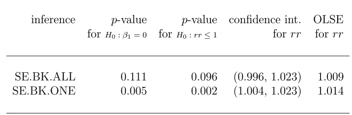
Table 5.1: Frequentist inferences for PM coarse linear effect.
inference p-value p-value confidence int. OLSE forH0:β1= 0 for H0:rr≤1 for rr for rr
SE.BK.ALL 0.111 0.096 (0.996, 1.023) 1.009 SE.BK.ONE 0.005 0.002 (1.004, 1.023) 1.014
Table 5.2 shows the inference results of the two EB procedures using ridge esti-mator. The ridge constant controlling the shrinkage of the parameter estimates are estimated as 137,580 and 151,657 by ”RDG.MLE” and ”RDG.GCV” respectively. Both of the EB procedures could be interpreted as implying a “positive” PM coarse linear mortality effect based on the category of Kass & Raftery (1995). Generally speaking, a posterior probability less than 0.5 for the hypothesis (H0 :β1 = 0) leads
posterior probabilities with the bounds: 0.5, 0.25, 0.05, and 0.01 corresponding to “weak”, “positive”, “strong” and “very strong” evidence for an association.
Table 5.2: Empirical Bayesian inferences for PM coarse linear effect.
inference post. prob credible int. post. mean for H0:rr≤1 for rr for rr
RDG.MLE 0.108 (0.995, 1.022) 1.008 RDG.GCV 0.122 (0.995, 1.021) 1.008
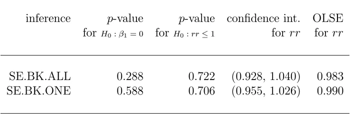
Inferences for PM fine linear effect
In contrast to PM coarse whose significant linear effect is well detected, all the suggested procedures fail to detect a significant PM fine linear effect. The frequentist S/E procedures for PM fine select tmax.l1, tmin.l1, tmin.l3, tg30, tmax.l1Q, t30Q
andt30.l1Qin addition to the 18 B-spline terms for basic model. Based on this basic model, the “SE.BK.ALL” procedure introduces all the 12 PM fine related variables to the model, while “SE.BK.ONE” selects p1f.l1 as the best PM fine variable. As seen in Table 5.3, the two inference procedures do not find any significant PM fine linear effect.
Table 5.3: Frequentist inferences for PM fine linear effect.
inference p-value p-value confidence int. OLSE forH0:β1= 0 for H0:rr≤1 for rr for rr
SE.BK.ALL 0.288 0.722 (0.928, 1.040) 0.983 SE.BK.ONE 0.588 0.706 (0.955, 1.026) 0.990
Table 5.4: Empirical Bayesian inferences for PM fine linear effect.
inference post. prob credible int. post. mean for H0:rr≤1 for rr for rr
RDG.MLE 1 (1, 1) 1
RDG.GCV 0.712 (0.913, 1.044) 0.981
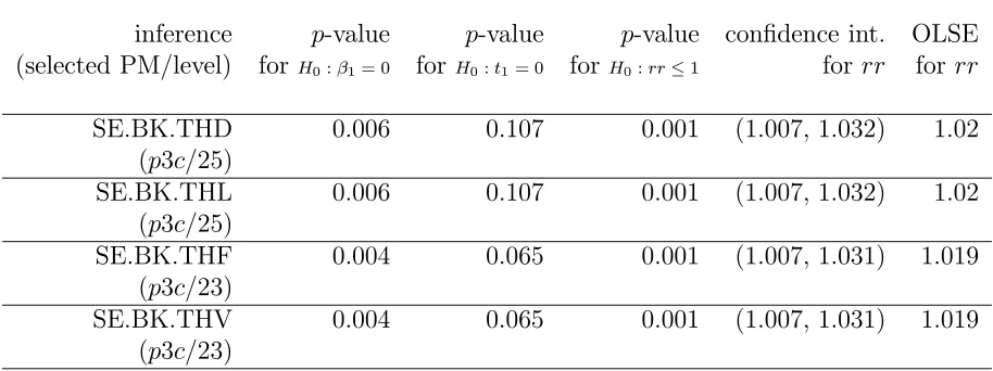
Inferences for PM coarse threshold effect
The four frequentist procedures described in Section 5.3 to catch the threshold effect of PM are applied. First, for the PM coarse, the basic model for the regional mortality selects tmax.l2, tmin, tg30.l2, tmax.l2Q, sh.l3Q in addition to the 18 B-spline terms for trend. Based on this basic model, the threshold terms along with the linear terms for PM coarse are selected by various strategies. (See the selection strategies in detail in Section 5.3.)
seem to come mainly from the linear effect of PM coarse.
Table 5.5: Frequentist inferences for PM coarse threshold effect.
inference p-value p-value p-value confidence int. OLSE (selected PM/level) for H0:β1= 0 forH0:t1= 0 for H0:rr≤1 for rr forrr
SE.BK.THD 0.006 0.107 0.001 (1.007, 1.032) 1.02 (p3c/25)
SE.BK.THL 0.006 0.107 0.001 (1.007, 1.032) 1.02 (p3c/25)
SE.BK.THF 0.004 0.065 0.001 (1.007, 1.031) 1.019 (p3c/23)
SE.BK.THV 0.004 0.065 0.001 (1.007, 1.031) 1.019 (p3c/23)
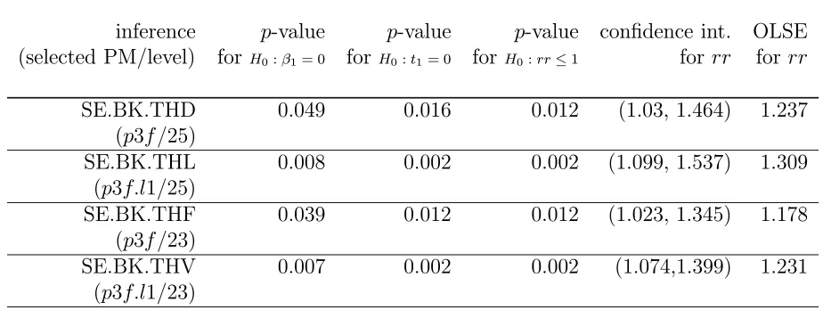
Inferences for PM fine threshold effect
Table 5.6: Frequentist inferences for PM fine threshold effect.
inference p-value p-value p-value confidence int. OLSE (selected PM/level) for H0:β1= 0 forH0:t1= 0 for H0:rr≤1 for rr forrr
SE.BK.THD 0.049 0.016 0.012 (1.03, 1.464) 1.237 (p3f/25)
SE.BK.THL 0.008 0.002 0.002 (1.099, 1.537) 1.309 (p3f.l1/25)
SE.BK.THF 0.039 0.012 0.012 (1.023, 1.345) 1.178 (p3f/23)
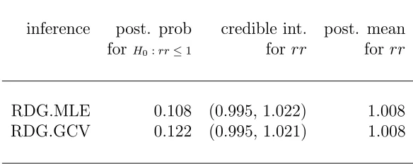
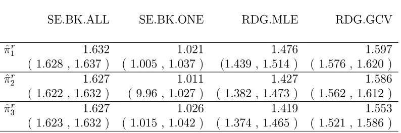
![Table 6.5: Relevant estimates and 95% confidence intervals for a performance measure ofthe Bayesian hypothesis test in the PM coarse linear model: Er(| pp.rr(X) − I[rr ≤ 1] |).](https://thumb-us.123doks.com/thumbv2/123dok_us/1426326.1175135/61.612.207.442.273.406/relevant-estimates-condence-intervals-performance-measure-bayesian-hypothesis.webp)