Abstract
WAN, BAOHONG. “Empirical Comparison of Simulation Models with Different
Input Data Structures.” (Under the direction of Dr. Nagui M. Rouphail.)
This thesis focuses on an empirical comparison of CORSIM and Paramics, two
commonly used traffic simulation models with different input data structures.
The case comparison was executed between a field-validated CORSIM model
and a fully calibrated Paramics network. These two models were constructed
based on the same physical network dataset, which was originally created for
the CORSIM simulation purposes. For those input data that were necessary
for Paramics, but not available in this dataset, estimations were performed
based on the known data and, sometimes, based on CORSIM default values.
Of these the most important one was the Origin-Destination (OD) matrix.
To enter traffic demand in Paramics, an OD matrix was derived using two
different methods, namely a statistical fitting method and a stochastic
assignment method. The feedback results from a Paramics test network
showed that the stochastic assignment method was more effective in deriving
One straightforward finding of the comparison was that Paramics generated
what appeared to be a larger percentage of unsuccessful runs than CORSIM.
That was possibly because Paramics created more link flow fluctuations with
the dynamic feedback traffic assignment algorithm; therefore, it had a higher
chance of spillback or blockage for overloaded links or turn movements.
A comparison of link flows in the two simulation models was executed based
on the sample replications after excluding outliers. It displayed that there were
some apparent link flow discrepancies between these two models. To ensure a
meaningful comparison of other selected traffic performance measures, two
critical corridors with minor vehicle flow discrepancies were selected as the
comparison sites.
By comparing the results on one corridor (NB LaSalle) , Paramics generated
fewer vehicle trips and a higher vehicle travel speed, while on the other
corridor (WB Ontario), the reverse occurred: although Paramics had fewer
vehicle trips on that corridor, it still produced lower vehicle speeds than
CORSIM.
The research suggests that empirical comparisons of simulation models with
performance that is at variance with CORSIM’s when using dynamic feedback
Biography
Baohong Wan was born in Shandong Province, China. He finished his
undergraduate study in transportation management engineering in Northern
Jiaotong University in 1995.
After graduation, he was hired as technical lecturer in Jinan Railroad Mechanical
School. In the following five years, he taught Freight Transportation Management
and Professional English to hundreds of railroad transportation staff.
In 2000 he was admitted to North Carolina State University to pursue graduate
study in transportation engineering in the Department of Civil Engineering. Under
the direction of Dr. Nagui Rouphail, he got a Master of Science degree in 2002.
Baohong’s major research interest is traffic capacity, delay and safety analysis
Acknowledgements
This thesis research was carried out under the direction of Dr. Nagui M. Rouphail,
Dr. Joseph Hummer and Dr. Stephen Roberts. The author would like to express
his special thanks to them.
Dr. Rouphail served as advisor for the author, for a candidate Master of Science
degree in transportation engineering in North Carolina State University. During
the past two academic years, his enthusiasm, valuable encouragement and
indispensable guidance made the fulfillment of this work possible.
Dr. Hummer, with his excellent engineering knowledge, taught the author to
study traffic problems from a practical perspective. Dr. John R. Stone presented
the author his first transportation class in NC State University. His broad
knowledge and humor made this class interesting and informative.
The ongoing research is under the direction of Dr. Jerome Sacks from Duke
University. The author is so grateful to him for his continuous support, sincere
advice and supervision during the work. It was Dr. Brian. B. Park who opened the
door for the author to this research.
This thesis is dedicated to my family; special thanks are given to my wife, Qing Li,
Table of Contents
List of Tables……… Vi
List of Figures………. Vii
Chapter 1: Introduction and Literature Review.………. 1
1.1 Traffic Simulation and Simulation Models……… 1
1.2 Model Selection and Comparison………. 3
1.3 Subject Models: CORSIM and Paramics ……… 5
1.4 Problem Statement.………. 9
1.5 Literature Review ……… 12
Chapter 2: Network Dataset and CORSIM Model ……… 18
2.1 Case Network Dataset ……… 18
2.2 CORSIM Network Modeling……… 23
2.3 CORSIM Network Outputs……….. 30
Chapter 3: OD Matrix Derivation……….. 33
3.1 Target OD Matrix and Solution Constraints………. 33
3.2 Statistical Fitting Method………. 36
3.3 Stochastic Assignment Method……….. 45
3.4 Adopted OD Matrix after Manual Adjustment……….. 49
Chapter 4: Paramics Network Construction, Calibration and Link Flow Comparison…..……… 54
4.1 Paramics Network Construction………. 54
4.2 Paramics Network Calibration……… 58
4.3 Paramics Link Flow Matching……… 63
Chapter 5: Simulation Output Comparison and Analysis………. 69
5.1 Outliers in CORSIM and Paramics Models ..………. 69
5.3 Comparison Results on NB LaSalle Corridor……….. 77
5.4 Comparison Results on WB Ontario Corridor……….. 80
5.5 Summary and Discussion.……….. 83
Chapter 6: Summary, Conclusions and Recommendations……… 85
6.1 Summary.……….. 85
6.2 Conclusions……….. 87
6.2 Recommendations………... 89
List of Tables
Table 1.1 Summary comparison of Paramics and CORSIM.……… 8
Table 2.1 Validation results for the CORSIM simulation network ……… 26
Table 3.1 Feasibility matrix
F
for the case network OD pairs.………… 35Table 3.2 OD traffic route matrix generated from Paramics.………. 38
Table 3.3 OD solution matrix from the statistical fitting method ...……… 41
Table 3.4 Summary of statistical fitting method solutions.………. 45
Table 3.5 OD solution matrix from the stochastic assignment method
……….. 48
Table 3.6 OD solution matrix after manual adjustment.………. 52
Table 3.7 Summary of feedback results with the adjusted OD ………… 53
Table 4.1 Comparison of link flows between CORSIM and Paramics … 64
Table 5.1 95% confidence intervals for the difference of mean link flow
rates .……… 73
Table 5.2 MOE comparison results on Northbound LaSalle Corridor
.………..……… 77
Table 5.3 MOE comparison results on Westbound Ontario Corridor
………..………. 80
Table 5.4 Comparison of through movement compositions on WB
List of Figures
Figure1.1 Map of the case study network ……… 11
Figure 2.1 CORSIM simulation network……….………... 24
Figure 2.2 Selected CORSIM links for validation ……… 25
Figure 2.3 Link trips validation results on Link 8 to 4..………. 27
Figure 2.4 Link stop time validation results on Link 8 to 4.………. 28
Figure 2.5 Link trips validation results on Link 5 to1……… 28
Figure 2.6 Link stop time validation results on Link 5 to 1……..………… 29
Figure 2.7 Link trips validation results on Link 10 to 9.……… 29
Figure 2.8 Link stop time validation results on Link 10 to 9……… 30
Figure 2.9 Plot of system queue time of the CORSIM simulation network.……… 31
Figure 3.1 Gridlock caused with the Solver OD……… 43
Figure 3.2 Single-source CORSIM network (WB Ontario) ……… 47
Figure 3.3 Round trips in CORSIM network runs ……… 49
Figure 4.1 Paramics simulation network.………... 57
Figure 4.2 Sensitivity test results on driver familiarity percentage ……… 60
Figure 4.3 Major/minor link classifications in Paramics network ………... 61
Figure 4.4 Link cost factors added to some undesirable links.…………... 63
Figure 4.5 Comparison of link flows between CORSIM and Paramics … 65 Figure 4.6 Linear relationship between the CORSIM and Paramics link flows.………. 65
Figure 4.8 Histograms of link flow ratios for the heavy loaded links ……. 67
Figure 4.9 Plot of important network links with link flow ratios
within (0.95,1) ………. 68
Figure 5.1 Animation of an outlier replication with traffic gridlock ……… 70
Figure 5.2 Two selected corridors for the comparison of traffic
Performance………..………. 72
Figure 5.3 Plot of vehicle miles comparison on NB LaSalle Corridor..….. 78
Figure 5.4 Plot of vehicle hours comparison on NB LaSalle Corridor.….. 79
Figure 5.5 Plot of vehicle speeds comparison on NB LaSalle Corridor.... 79
Figure 5.6 Plot of vehicle miles comparison on WB Ontario Corridor.….. 81
Figure 5.7 Plot of vehicle hours comparison on WB Ontario Corridor….. 82
Chapter 01: Introduction and Literature Review
1.1 Traffic Simulation and Simulation Models
Traffic Simulation
Traffic simulation refers to the process of designing and creating a computerized
model of an existing or proposed transportation system, for the purpose of
conducting numerical experiments to give users a better understanding of the
behavior of that system for a given set of conditions (Kelton, 2001). Simulation is
increasingly being used in the transportation and traffic engineering field, not only
because of its strength in analyzing complex systems requiring a large number of
calculations, but also because of its capabilities in providing users statistical
measures of effectiveness and, more recently, visualized demonstration of target
traffic scenarios.
The emergence of low-cost modern computers with higher computation speeds
and larger storage capacity has extended the application of traffic simulation to
small project analysis and routine traffic management. Rapid development in
computer simulation software provides users various modeling choices to choose
Traffic Simulation Models
There are several ways to classify traffic simulation models, but one useful way is
along three dimensions (Prevedouros, 2000):
• Microscopic, macroscopic or meso-scopic models. Microscopic simulation
models include CORSIM (FHWA, 1997), PARAMICS (Quadstone, 1999),
VISSIM (PTV, 1999), etc. Macroscopic simulation models include
CORFLO (FHWA, 1997), FREFLO (Payne, 1979), and meso-scopic
models include DYNASMART (FHWA, 2000) and TRANSIMS (LANL,
1998).
• Stochastic or deterministic models. CORSIM, VISSIM, INTEGRATION
(Van Aerde, 1995), etc, are stochastic models, while DYNASMART, HCS
(McTrans, 2000), and TRANSYT7F (McTrans, 1999), are deterministic
models.
• Continuous or discrete models. Most traffic simulation models are discrete
changing models running at fixed time steps (typically at 1 second interval
or less).
From the perspective of traffic demand input data, traffic simulation models can
be classified into flow-based simulation models (for example, CORSIM,
Flow-based traffic simulation models are designed mainly to reproduce link
performance. Such models use entry volumes and turn percentages as the traffic
input demand. Once inside the network, vehicles are assigned to downstream
links according to prescribed turning probabilities.
By contrast, path-based simulation models concentrate on reproducing network
trip making behavior. Therefore, Origin Destination (OD) matrices represent the
input traffic demand. In this kind of models, traffic assignment is performed using
specified routing algorithms based on minimizing total travel costs, or some
variation thereof.
1.2 Model Selection and Comparison
Simulation model selection will affect not only the network modeling process and
the required labor, but also the simulation results and, therefore, any user
conclusions or recommendations. The selection of a simulation model should be
based on its capability of producing accurate results as well as the feasibility of
its use for specific applications.
Model comparison can assist users in making correct choices with regards to
model selection. Performed at different levels, simulation model comparison
Besides assessing some general considerations, including modeling cost, speed,
system needs, etc, a conceptual comparison evaluates the capabilities of each
model. Material for this kind of comparison is mostly found in the user guides of
the subject simulation models. The conceptual comparison is an efficient way to
understand the modeling features and functionalities of different simulation
models in a short time.
By contrast, the empirical comparison is targeted at answering higher-level
questions such as “how” and “how well” these models function. To achieve this
purpose, the selected traffic simulation models are separately applied to the
same traffic network. A side-by-side visual comparison is regularly carried out as
well as a statistical comparison of run outputs from different simulation networks.
The empirical comparison of simulation models with different input data
structures, as for example, a flow-based simulation model versus a path-based
simulation model, is complicated in that it requires traffic demand data in different
structures. Traffic data in the form of entry volumes, as well as origin-destination
matrices, are both required as inputs to the simulation models to be compared.
In the real world, OD matrix demands are usually very difficult to gather in the
field because of technical and cost reasons. In a license-plate analysis, for
addition, the large costs incurred in recording-station construction and car-plate
data processing discourage many traffic researchers (Lu, 1998).
Since link flow and turn movement data are relatively cheaper and easier to
acquire in the field, considerable research has been devoted to deriving OD
matrices from these easily acquired traffic data. That literature is reviewed in
section 1.5 of this chapter.
1.3 Subject Models: CORSIM and Paramics
The goal of this research is to develop a method to empirically compare traffic
simulation models with different input structures. As an illustration, CORSIM and
Paramics, two commonly used traffic simulation models that typify flow-based
models and path-based models, respectively, are applied to a case network. A
brief description of each traffic simulation model is given below.
CORSIM
The CORSIM (CORridor SIMulation) model was rooted in the development of
DYNASIM in the 1970’s. It is now the core part of the Traffic Software Integrated
System (TSIS) package, which is sponsored by the Federal Highway
most recent version of CORSIM, version 5.0, was released in 2001 as part of
TSIS 5.0.
CORSIM uses entry volumes as the input form for traffic demand, and performs a
stochastic-assignment at each intersection. Since the prescribed turning
probabilities are taken to be independent of the network origins, vehicles from
different origins have a similar likelihood of being assigned to a specified
downstream link. The major objective of CORSIM is to reproduce link traffic
performance, such as vehicle trips, vehicle speeds, etc, and not worry about trip
or path based characteristics.
Nationwide applications illustrate that after careful calibration, CORSIM is able to
reproduce link performance and therefore provide users with useful information
for traffic scenario analysis. However, the stochastic assignment method (which
is based on prescribed turning probabilities only) does prevent CORSIM from
carrying out an evaluation of traffic scenarios with significant network changes
(for example, adding or dropping links, or altering existing links, which will
unavoidably result in different trip route patterns, and therefore changed turning
probabilities). It also doesn’t handle “trip-based” algorithms such as bottleneck
Paramics
The Paramics (PARAllel MICroscopic traffic Simulator) is an advanced suite of
software tools for microscopic traffic simulation. It has its root in the cooperate
research of SIAS Limited and the University of Edinburgh’s Parallel Computing
Center (EPCC) in Scotland. In 1996 Quadstone Limited developed Paramics 1.0
for commercial use. Quadstone Paramics version 3 build 7 was released in 2001.
Paramics uses OD matrices as the input form for traffic demand. It provides a
number of traffic assignment algorithms from which users can choose. To
reproduce the network performance properly, users are required to choose the
traffic assignment method that provides the best fit to observed data, and to
calibrate the network assignment parameters to render the vehicle routing
behavior as close to the “reality” as possible.
Since Paramics provides a dynamic feedback algorithm in the traffic assignment
model, it can ostensibly be used to analyze traffic performance of the scenarios
with drastic network changes, which could result in different traffic assignment
patterns. This feature also enables Paramics to simulate Intelligent
Transportation System (ITS) applications in some transportation networks. For
example, Paramics 1.5 was recently used in the ITS study by the California
Partners for Advanced Transit and Highways (PATH) program. (Abdulhai, et al,
As a simulation model originating in Europe, Paramics also has attracted
interests from many U.S. researchers because of its powerful roundabout
simulation tools. For example, an operational and functional design evaluation for
Lane County, Oregon (www.paramics-oneline.com/projects/Kittelson) was
carried out in Paramics. However, because of its emphasis on European design,
the default vehicle and driver characteristics in Paramics had to be carefully
recalibrated to U.S. conditions.
A summary comparison of the main feature of CORSIM and Paramics is shown
CORSIM Paramics
Vendor McTrans Center, FL Quadstone Limited, UK
System requirements Microsoft Windows 95,
Windows 98,Windows NT 4.0
or Windows 2000
Windows NT/95/98/2000,
or Sun Microsystems/Solaris,
or Silicon Graphics/IRIX
Classification Microscopic, stochastic, flow-based Microscopic, stochastic, path-based
Batch mode running CORSIM script,
runcor.exe
Paramics Processor,
modeller-batch.exe
Graphical input editor TRAFED (TRAF Editor) Paramics Modeller
Animation Processor TRAFVU (TRAF Visualization Utility) Paramics Modeller, Analyser
Statistical Outputs TRAFVU Paramics Analyser
Input Demand Entry volumes OD Matrix
Traffic Assignment Stochastic assignment based
On turning probabilities
All-or-nothing (AON) assignment;
Probabilistic AON assignment;
Dynamic feedback algorithm
Traffic Control Signal, stop/yield sign,
ramp metering, roundabouts
Signal, priority control, roundabouts
Incident Simulation Yes. Yes.
Emission Analysis Yes. Paramics Monitor
Open Structure No. Paramics Programmer for API
(Application Programming Interface)
1.4 Problem Statement
Objectives and Scope
The objectives for this research are summarized as follows:
1. To develop a consistent input data structure for simulation model
construction and comparison;
2. To identify similarities and differences between Paramics and CORSIM
models; and
3. To validate the Paramics model.
To ensure a meaningful comparison, a Paramics network needs to be
constructed based on the same network dataset as the CORSIM model.
Although Paramics is very similar to CORSIM in most of its network input data,
there are still some major differences between these two models’ input structures,
most noticeably, the specification of an OD matrix as the traffic input demand in
Paramics. As the network dataset was originally constructed for the CORSIM
model, no OD data were readily available. Therefore, some input data needed to
be calculated or estimated from other known traffic data.
Consequently, because of the limitation of the original network dataset and the
difficulty in collecting field OD data, the Paramics model was constructed based
(b) calculated or estimated data from the CORSIM dataset, and (c) CORSIM
default values which have been validated for the case study urban network.
Case Study
A medium-size urban network, which is located in the central part of the city of
Chicago, served as the case study. This case network shown in Figure 1.1
includes 24 signalized intersections, 8 un-signalized intersections, 56
surface-street segments and 2 freeway segments. The target simulation time period is
Thursday, May 27th, 2000, 17:00 to 18:00 PM, which is a typical evening peak
hour period. About 13,000 vehicles travel through this network during the subject
time period.
Figure1.1: Map of the case study network
As this research was a continuing part of a project aimed at optimizing traffic
signal plans for the case network using CORSIM simulation (Sacks, et al, 2000),
a network dataset for inputs to CORSIM had already been constructed, and a
CORSIM network had already been constructed, calibrated and validated.
In order to perform the empirical comparison, Paramics was applied to this traffic
network. An OD matrix was derived from known traffic data, such as entry
volumes, turning percentages, link volumes, etc, to enter traffic demand in
Paramics. Outputs from independent replications of the simulation networks in
CORSIM and Paramics are gathered and compared in order to draw conclusions
and make recommendations.
Thus, the following tasks were carried out:
1. Derive a Paramics OD matrix from known traffic information;
2. Construct and calibrate the Paramics simulation network; and
3. Design and carry out output comparisons between the two simulation
1.5 Literature Review
The two key research problems of this thesis, application and evaluation of traffic
simulation models and derivation of OD matrices from traffic count information,
have been explored by many investigators. Some key findings are summarized
below.
Application and Evaluation of Traffic Simulation Models
As a quasi-official traffic simulation model sponsored and used by FHWA,
CORSIM has been widely used in many traffic-engineering studies. Daigle, et al
(1998) used CORSIM for the simulation of two freeway reconstruction
alternatives in Oklahoma City. The simulation was successful in identifying
problem areas and in assisting transportation professionals in selecting a
preferred alternative. Another application example was by Maze, et al (1998).
CORSIM was used to simulate arterial traffic operations along US 61 corridor in
Burlington, Iowa. The intersection-level performance measures from the
simulation outputs enable researchers to compare five alternative models to the
base model. A more recent application of CORSIM 5.0 by Luh (2001) to two
projects in Florida included the modification of an existing interchange and the
Sacks, et al, (2000) employed CORSIM to analyze different approaches to
optimizing traffic signal plans. They described a general process of a statistical
based validation of traffic simulation models, and concluded that CORSIM,
though not perfect, was effective in evaluating signal plans of urban networks.
Rouphail, et al, (2000) and Park, et al, (2000) proposed a stochastic signal
optimization method based on a genetic algorithm (GA) that interfaced with
CORSIM. They found that the solution from the method was superior to an
optimum TRANSYT-7F (T7F) plan.
Although Paramics is relatively new simulation software, it is now used in more
than twenty countries throughout the world. In the United States, one typical
application of Paramics was for modeling Intelligent Transportation System (ITS)
as part of the California Partners for the Advanced Transit and Highways (PATH)
program. Abdulhai, B, et al (1999) reported the phase I, calibration and
validation, of simulation of ITS on the Irvine Field Operational Test (FOT) area
using Paramics 1.5 scalable microscopic traffic simulator. In this research
Paramics was thoroughly evaluated for modeling ITS. It was concluded that
Paramics is an excellent ‘shell’ or ‘framework’ for a comprehensive and extensive
transportation simulation laboratory because of its high performance and
scalability. In another ITS study, Liu, et al. (2000) reported some developments
of Paramics Application Programming Interface (API) programs for actuated
Sahraoui, A. et al. (2002) proposed a methodology based on a hybrid simulation
approach for microscopic simulation that was intended to explore two critical
aspects, calibration/validation methodology and integration of path dynamics.
The Paramics microscopic simulation was integrated with the DYNASMART
macroscopic model to enhance the evaluation of traffic information-based routing
behavior in the Advanced Traffic Management Information Systems (ATMIS).
An important exercise of simulation model comparison was recently performed In
Europe. Entitled the Simulation Modeling Applied to Road Transport European
Scheme Tests (SMARTEST) (1996-1999), thirty-two most commonly used traffic
simulation suites were evaluated from different aspects, including the modeling
functions available, objects and phenomena modeled, indicators provided, and
other properties. In the United States, Boxill and Yu (2000) presented an
evaluation of more than 80 traffic simulation models in an attempt to evaluate the
potential application of ITS equipped networks. They found that CORSIM and
INTEGRATION appeared to have the highest probability of success, whereas by
adding more calibration and validation, the AIMSUN2 and Paramics would be
brought to the forefront for use with ITS applications.
In an empirical comparison of simulation models, Wang and Prevendouros (1997)
compared performance of Integration, CORSIM and WATSim by applying them
to three small networks in Honolulu. They found that INTEGRATION was least
lane-changing behavior; WATSim needed the least calibration for producing good
results, but its universal car-following parameters were undesirable. Bloomberg
and Dale (2000) compared the VISSIM and CORSIM simulation models on a
congested network. The consistency and reasonableness of the simulation
results led them to believe that it might be practical to use more than one model
for make the analysis more reliable, and the results more defensible.
OD Estimation
OD estimation is a well-established research topic in the field of transportation
engineering as well as operation research. The OD estimation problem can be
attacked from three different approaches, namely a traffic modeling approach, a
statistical inference approach and a gradient approach (Abrahamsson, 1998).
The traffic modeling approach derives a ”minimum information” OD matrix to
achieve entropy maximization. Zuylen and Willumsen (1980) initially explored this
approach, based on a gravity trip distribution model. Fisk (1988) extended this
model by introducing user-equilibrium conditions as constraints on congested
transportation networks.
The statistical inference approach includes several different techniques, as
different objective functions can be used. Spiess (1987) proposed an algorithm of
maximizing the likelihood between the observed traffic counts of the target OD
their finding in estimating OD matrix using generalized least square (GLS)
method with the assumption of proportional trip assignment. Maher (1983) also
assumed proportional assignment in his Bayesian inference algorithm to estimate
an OD matrix. Sherali (1997) explored this approach using a least norm estimator
since it was intuitively more robust to outliers.
Among all different statistical objective functions, the generalized least square
method was most frequently cited in recent research. For example, Dixon and
Rilett (2002) examined a generalized least square method and a Kalman filtering
method using automatic vehicle identification count data.
The gradient-based solution technique takes an OD matrix estimate as an initial
solution, and then attempts to reproduce the traffic counts by iteratively adjusting
OD pairs. It was separately explored by Spiess (1990), Yang, et al., (1992), and
Chen (1994). This technique is proposed to solve the optimization problem for
Chapter 02: Network Dataset and CORSIM Network
In this chapter, a network dataset containing different inputs to the simulation
models is presented in Section 2.1. The CORSIM simulation network is
described in Section 2.2, and outputs from the CORSIM network are summarized
in Section 2.3.
2.1 Case Study Network Dataset
A case network dataset was prepared for the modeling using CORSIM and
Paramics. This dataset contained field data, including network geometry, traffic
control, traffic demand, vehicle and driver attributes, and some other attributes.
As mentioned in Chapter 1, since this research was the continuation of a project
aimed at optimizing signal plans for this same case network using CORSIM
simulation, most network data collection for the CORSIM inputs had already
been done with the assistance of the Chicago Department of Transportation
(DOT). Since this dataset would also be applied to the Paramics model, it is
Network Geometry Data
Network geometry data include street geometry data, intersection geometry data,
and some other geometry data.
Key link geometric horizontal alignment data were gathered in details in the field.
Stop-bar-to-stop-bar distances, and lengths of turning pockets were manually
measured as important street lateral characteristics. The numbers of traveling
lanes and pocket lanes were counted to determine street width.
For the geometry data that were difficult to gather in the field, some default
values were assumed. These values included lane widths of 12 feet, and the link
sections that were assumed to be straight. As the terrain was level, grades for all
streets were assumed to be zero. Since none of the parking lots appeared to
have a significant effect on this area, all streets were assumed not to have any
driveway. These assumptions simplified the modeling process and did not
Some intersection data, such as intersection length, width, turning radius, were
assumed to have minor effect on the operation of the test network, although they
were indeed used in some simulation studies as part of the control parameters.
In this case study, no detailed intersection geometry data were gathered. No
sight distance data were gathered in the field either.
Network Traffic Control Data
Network traffic control data include both intersectional traffic control data and
sectional traffic control.
For the intersectional traffic control, the Chicago Department of Transportation
(CDOT) provided the detailed signal plan for the signalized intersections, as well
as sign types and locations for the un-signalized intersections. At the signalized
intersections, right turn on red (RTOR) or left turn on red was allowed at most
intersections in the target area, except for one turn movement from a surface
street to a freeway section.
Sectional traffic control regulations including lane usage, lane changing and
design speeds, were gathered for each street. Types and locations of warning
signs for sectional traffic were not gathered since they are seldom being
On-street parking was not allowed throughout the case network, but during the
target simulation time period, there were actually a few sections on some streets
occupied by illegally parked vehicles. Since both simulation models don’t have
parking-lane simulating functions, lengths of actual parking lanes were recorded
and corresponding parts of these lanes in the simulation networks were closed to
traffic.
Network Traffic Input Data
As the traffic demand inputs to the simulation network, entry volumes and turning
probabilities were manually gathered for the target time period. However, no OD
traffic data were gathered in the field during that period.
In the network boundary area, entry volumes and turning movement counts were
gathered manually, whereas inside the network, turning counts were gathered
from videotapes, which were recorded from seven different angles covering most
parts of the study area.
To enter the percentages of different vehicle types, heavy vehicle counts were
done at the same time as the entry link counts. Buses were counted separately
Volumes of pedestrians were not counted in the field since almost all
intersections had only low pedestrian traffic. Instead, two locations were
estimated to have no pedestrian traffic, while others were estimated to have low
pedestrian volumes. No bicycle data were gathered for the case network since
the bicycle traffic was low throughout the network.
Network Vehicle Composition and Driver Attributes
In microscopic traffic simulation networks, vehicles are the simulation entities
traveling through the network. As a major characteristic of the vehicles, the heavy
vehicle percentage was gathered in the field. However, detailed vehicle
composition data (for example, percentage of heavy vehicles that are single-unit
trucks), were not gathered since they are too difficult to be measured. Therefore,
when constructing the simulation model, default vehicle composition percentages
were used.
Performance of an individual vehicle depends not only on the vehicle
characteristics, but also on the driver attributes. Unfortunately, due to the same
reasons as the vehicle composition data, no driver attribute data could be
gathered in the field. The necessary driver attribute data for CORSIM and
Paramics modeling include driver aggression, driver awareness, driver sensitivity
As a usual way to deal with driver studies, driver attributes were assumed to
follow normal distributions, although in CORSIM some discrete distributions are
used as simplified approximations.
Driver familiarity percentage is an important parameter to the traffic assignment
algorithms in Paramics. Familiar drivers have different coefficients in the
calculation of costs on minor streets. Moreover, familiar drivers are able to
change their routes whenever they are experiencing extra delay, while unfamiliar
drivers would remain on the preset routes, even when they are delayed by
congestion for a long time.
The driver familiarity percentage for this case network could not be directly
gathered in the field. The calibration of this percentage will be discussed in
Chapter 5.
2.2 CORSIM Network
The CORSIM network was already constructed, calibrated and validated in a
previous study for optimizing the signal plan using simulation. Details of the
Network Representation
The CORSIM simulation network is comprised of 166 network links, 56 network
nodes, and 47 dummy entry nodes for the origins of vehicle inputs. The CORSIM
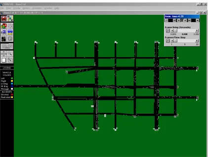
network is shown in Figure 2.1.
Figure 2.1: CORSIM simulation network
CORSIM default values were used for the vehicle and driver characteristics. Two
noticeable calibration parameters having significant effect on capacity and delay
values in CORSIM, which were respectively 2.0 seconds and 1.8 seconds, were
used; and the distribution forms of the individual vehicle attributes were
approximately normal.
Model Validation
The validation was executed by comparing field data at several key links to
CORSIM predictions. The criteria for selecting these links were 1) availability of
field data, and 2) whether they were key to the overall performance of the
network from a transportation standpoint.
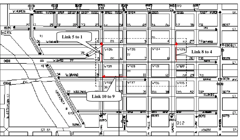
Figure 2.2: Selected CORSIM links for validation
Link 8 to 4 Link 5 to 1
• Link 8 to 4, Northbound LaSalle Street from Ohio Street to Ontario Street,
• Link 5 to 1, Northbound Orleans Street from Ohio Street to Ontario Street;
and
• Link 10 to 9, Westbound Grand Street from Franklin Street to Orleans
Street.
The validation process was based on one hundred replications of CORSIM runs.
The number of replication was statistically large enough to yield a relative short
confidence interval around the mean.
The visual validation of individual simulation run showed that gridlock (network
run failure because of vehicle spillback effect) appeared in some replications.
These replications yielding apparent deviant outputs because of gridlock are
referred to as outliers. Details about gridlock and outliers are discussed in
Chapter 5. After excluding outliers, ninety-eight effective replications were
summarized for statistical validation.
Mean link trips and mean stop time per vehicle were used as major measures of
effectiveness (MOE) for validation. Summary results of these statistics are
Link Trips Link Stop Time per Vehicle CORSIM Link Street Name CORSIM Mean (1) CORSIM STDEV (1) Field
Value Ratio (2)
CORSIM
Mean (1)
CORSIM
STDEV (1)
Field
Value Ratio (2)
8 to 4 NB LaSalle 1616.8 23.4 1636.0 0.99 20.7 3.4 21.5 0.96
5 to 1 NB Orleans 1069.2 28.7 1078.0 0.99 9.8 1.5 9.1 1.08
10 to 9 WB Grand 1009.3 34.0 1117.0 0.90 22.5 7.4 24.4 0.92
Table 2.1: Validation results for the CORSIM simulation network
Note: 1) Based on 98 replications of CORSIM runs.
2) CORSIM mean (1) divided by field value.
As can be seen in Table 2, all CORSIM statistics are within 10 percent variance
of the field values.
Student t-tests were not performed for the validation, since the mean values of
the simulation outputs would not necessarily be the field observed values
because of observation variability. Instead, direct plots of histograms for MOEs of
interest were used and visual comparison with field observation was performed.
Plots of link trips and link stop time for Link 8 to 4, Link 5 to 1, and Link 10 to 9,
Figure 2.3: Link trips validation results on Link 8 to 4
Note: Arrow shows field value
Figure 2.4: Link stop time validation results on link 8 to 4
Note: Arrow shows field value
Validation Results of Link Stop Time on Link 8=>4
0 5 10 15 20 25 30 35 40
10 12.5 15 17.5 20 22.5 25 27.5 30 32.5 35 More
Link Stop Time (sec/veh)
Fr
equency
Validation Results of Link Trips on Link 8=>4
0 5 10 15 20 25 30 35
1520 1540 1560 1580 1600 1620 1640 1660 1680 1700 1720 More
Link Trips
Fr
Figure 2.5: Link trips validation results on Link 5 to 1
Note: Arrow shows field value
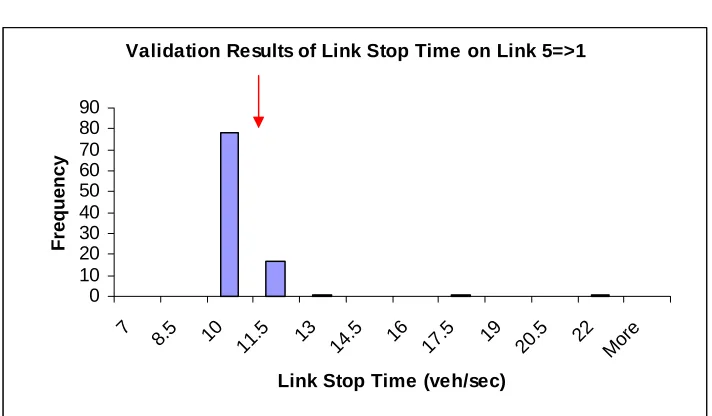
Figure 2.6: Link stop time validation results on link 5 to 1
Note: Arrow shows field value
Validation Results of Link Trips on Link 5=>1
0 5 10 15 20 25 30 35
960 980 1000 1020 1040 1060 1080 1100 1120 1140 1160 More
Link Trips
Fr
equency
Validation Results of Link Stop Time on Link 5=>1
0 10 20 30 40 50 60 70 80 90 7
8.5 10 11.5 13 14.5 16 17.5 19 20.5 22 Mor
e
Link Stop Time (veh/sec)
Fr
Figure 2.7: Link trips validation results on Link 10 to 9
Note: Arrow shows field value
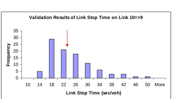
Figure 2.8: Link stop time validation results on link 10 to 9
Note: Arrow shows field value
Validation Results of Link Trips on Link 10=>9
0 5 10 15 20 25 30 35
850 875 900 925 950 975 1000 1025 1050 1075 1100 More
Link Trips
Fr
equency
Validation Results of Link Stop Time on Link 10=>9
0 5 10 15 20 25 30 35
10 14 18 22 26 30 34 38 42 46 50 More
Link Stop Time (sec/veh)
Fr
The validation results demonstrated that the CORSIM network reproduced link
trips and link stop times successfully, although in one link (Link 10 to 9) it
produced link trips that were 10 percent higher than the field value.
2.3 CORSIM Network Outputs
The outputs from the CORSIM simulation network are briefly summarized below.
The statistics of interest here are percentage of outliers and system queue time.
The percentage of outliers is frequently used to indicate network stability and
model run effectiveness, assuming that the gridlocks are not caused by
inadequate capacity or network coding errors. The criterion to judge outliers is if
the system queue time exceeds a certain threshold, which are 300 vehicle hours
in this research. Only two of the one hundred replications had system queue time
more than 300 vehicle hours. This demonstrated that the CORSIM simulation
network was a fairly stable model.
System queue time for the overall network was employed as the global measure
of effectiveness (MOE) to characterize the system congestion level. The plot of
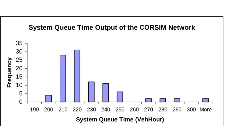
Figure 2.9: Plot of system queue time of the CORSIM simulation network
Note: 1) Based on one hundred replications of CORSIM runs
2) The right-most bar corresponds to data from 2 outliers
As shown in this histogram plot, the CORSIM network system queue time is
right-skewed and the mode is between 210 and 220 vehicle-hours. The mean,
median and standard deviation of system queue time are 225, 214 and 36
vehicle-hours, respectively.
Some other system-level statistics including network throughput, system stop
time, system vehicle hours, etc, and local level statistics such as corridor or link
trips, stop times, vehicle hours, were also gathered. These results will be
discussed in Chapter 5.
System Queue Time Output of the CORSIM Network
0 5 10 15 20 25 30 35
190 200 210 220 230 240 250 260 270 280 290 300 More
System Queue Time (VehHour)
Fre
que
nc
Chapter 03: OD Matrix Derivation in Paramics
In this chapter, the OD matrix derivation methods and processes are described in
detail. Section 3.1 provides criteria for evaluating OD solutions from different
derivation methods. The statistical fitting method and stochastic assignment
method are described in Sections 3.2 and 3.3. In Section 3.4 the adopted OD
solution by manual adjustment is presented.
3.1 Target OD Matrix and Solution Constraints
OD derivation Methods and Evaluation
As mentioned in the literature review in Chapter 1, depending on different
available data, the target OD matrix could be estimated using various methods.
One criterion to evaluate the solutions from different derivation methods is the
ability to reproduce link flows. If the OD matrix is fed to a well-tuned Paramics
model, (a) the number of outliers (i.e., runs with gridlock) should be small
(because it is small in CORSIM), and (b) the link flow discrepancies between
Paramics and CORSIM should to be small too. Paramics was tuned to have a
low mean driver reaction time (0.5 sec) and low mean car-following headway (0.7
In this research, based on the available data, two different OD matrix derivation
methods were studied: a statistical fitting method and a stochastic assignment.
The statistical fitting method was based on given (by CORSIM) link volumes and
derived traffic assignment routes, while the stochastic assignment method was to
determine the target OD matrix from given entry volumes and turning
probabilities (the needed inputs to CORSIM). The number of outliers and the
discrepancy between Paramics link flows and CORSIM flows were used to
compare the two methods.
Constraints on the OD Solutions
Successful OD matrix solutions must satisfy feasibility constraints and
entry-exit-volume constraints to achieve reasonable results.
• Feasibility Constraint
The feasibility constraint is to assign traffic demand only to those feasible OD
pairs. For this case network, trips between some OD pairs are infeasible, so that
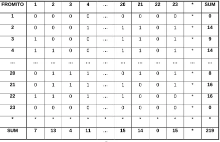
for any solution matrix, the corresponding cell values should be 0. Summarizing
the feasibilities for each OD pair leads to a feasibility OD matrix
F
, in whichFROM\TO 1 2 3 4 … 20 21 22 23 * SUM
1 0 0 0 0 … 0 0 0 0 * 0
2 0 0 0 1 … 1 1 0 1 * 14
3 1 0 0 0 … 1 1 0 1 * 9
4 1 1 0 0 … 1 1 0 1 * 14
… … … …
20 0 1 1 1 … 0 1 0 1 * 8
21 0 1 1 1 … 1 0 0 1 * 16
22 1 1 0 1 … 1 0 0 0 * 16
23 0 0 0 0 … 0 0 0 0 * 0
* * * * * * * * * * * *
SUM 7 13 4 11 … 15 14 0 15 * 219
Table 3.1: Feasibility matrix
F
for the case network OD pairsTable 3.1 shows part of the feasibility matrix
F
for the case network OD pairs.Therefore, vehicle trips will only be assigned to the 219 feasible OD pairs.
• Entry-Exit-Volume Constraint
This constraint requires a match between any OD solution and the known
marginal entry and exit link volumes. Origin and destination volumes for all
demand zones can be obtained from the field traffic counts at the entry and exit
links. Thus, the rows and sum of columns of the target OD matrix solution should
∑
∑
= ==
=
n i j j i n j i j iD
od
O
od
1 , 1 ,Where
o
d
i,j denotes the unknown OD traffic demand from zone i to zone j, Oidenotes traffic origin demand from zone i, Dj denotes traffic destination demand to zone j, and n denotes the number of demand zones in the case network.
The transpose of the origin vector
O
and the destination vectorD
for the casenetwork are shown below.
(
)
)
3878
0
712
299
...
88
5
126
15
(
0
1850
453
47
...
50
43
232
0
=
=
T TD
O
3.2 Statistical Fitting Method
Approach
The statistical fitting method was based on given traffic link volumes and routes
associated with each OD pair. Provided that an OD traffic routing algorithm is
available, for each OD matrix solution, the corresponding “theoretical” link
volumes could be solved. Since the target OD matrix always generates
generates the least matching error, therefore, could be used as an approximation
of the target OD matrix. Thus, the OD estimation problem can be solved as a
constrained nonlinear programming problem.
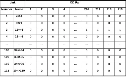
• Step 1: Generate the traffic route matrix
R
A calibrated Paramics network using the static assignment option (where familiar
drivers won’t change their routes during the simulation) was used in the OD trip
routing algorithm. As there were 219 feasible OD pairs and 111 effective network
links, the routing algorithm was represented by a traffic route matrix
R
, whichwas an
111
×
219
identity matrix where cell (i, j) was assigned a value of 1 iftraffic between OD pair i traverses link j, 0 otherwise.
The Paramics network was run with a 0-1demand matrix, which was constructed
by placing unit demand for all feasible cells. Since each unit trip stood for a
different OD pair, the traffic route matrix
R
was constructed through recording allthe resulting traffic routes in Paramics. Part of a generated route matrix
R
isLink OD Pair
Number Name 1 2 3 4 … 216 217 218 219
1 2=>1 0 0 0 0 … 0 0 0 0
2 5=>1 0 0 0 0 … 0 0 0 0
3 13=>1 0 0 0 0 … 1 1 1 1
4 23=>1 0 0 0 0 … 0 0 0 0
… … … …
108 32=>94 0 0 0 0 … 0 0 0 0
109 33=>95 0 0 0 0 … 0 0 0 0
110 34=>96 0 0 0 0 … 0 0 0 0
111 10=>110 0 0 0 0 … 0 0 0 0
Table 3.2: OD traffic route matrix generated from Paramics
• Step 2: Generate the theoretical link volume vector
T
For each possible OD matrix solution, a solution vector
S
is defined as thevector containing 219 corresponding feasible OD pair values. The “theoretical”
link volume vector
T
is defined by:)
(
219
1 ,
∑
=×
=
i
i i j
j
R
s
• Step 3: Generate the empirical link traffic volume vector
E
An empirical link traffic volume vector
E
, which was composed of 111 knownlink volumes, was gathered from the validated CORSIM network. To account for
the randomness in CORSIM replications, ten runs were performed and the link
counts were gathered from the replication having the median system queue time.
One hundred and eleven link traffic volumes were collected as the empirical
values to match.
• Step 4: Establish the objective function
The error between the theoretical and empirical link volumes,
2 111
1
)
(
∑
=−
=
jj
j
E
t
SSE
, where SSE stands for Sum Square Error of link volumes, is to be minimized by
choice of
S
. It is a nonlinear programming problem that requires the use of anoptimization algorithm. The resulting problem included 219 adjustable variables
that were subject to the origin/destination flow constraints. As a common tool for
small linear or non-linear programming problems, Microsoft Excel Solver was
• Step 5: Combine familiar driver and unfamiliar driver solutions
Since the static assignment option was used in Paramics, the OD routing matrix
was actually solved based on an all-or-nothing traffic assignment method.
Paramics generation was executed under two different assumptions, one using
100% familiar drivers and the other using 100% unfamiliar drivers, to account for
the multiple-route behavior between some OD pairs. Thus, two routing matrices,
)
(
F
R
for familiar drivers andR
(
U
)
for unfamiliar drivers, were created. Thesetwo routing matrices were applied to the entire derivation process separately and
the solutions were ultimately combined with a 40/60 split for unfamiliar/familiar
driver solutions to generate a final solution for application.
FROM
\TO 1 2 3 4 5 6 7 8 9 10 11 12 13 14 15 16 17 18 19 20 21 22 23 * SUM 1 0 0 0 0 0 0 0 0 0 0 0 0 0 0 0 0 0 0 0 0 0 0 0 * 0
2 0 0 0 10 57 0 0 0 0 0 0 26 0 43 0 8 14 0 38 10 26 0 0 * 232
3 2 0 0 0 14 0 0 0 0 0 0 0 0 0 0 0 0 0 11 0 16 0 0 * 43
4 1 0 0 0 0 8 0 2 0 0 0 4 0 0 0 0 0 0 8 0 20 0 7 * 50
5 4 12 0 0 0 0 0 0 0 38 0 57 0 12 0 0 6 19 0 58 8 0 628 * 841
6 1 1 0 45 0 0 0 1 0 24 0 68 0 1 1 0 0 0 0 0 0 0 43 * 186
7 0 0 0 0 49 0 0 0 0 135 0 89 0 13 1 5 206 1 0 0 0 0 50 * 549
8 4 0 0 0 0 8 0 0 0 0 0 32 0 125 35 527 29 1 1 8 9 0 192 * 970
9 0 0 0 0 22 87 0 0 0 0 0 0 0 174 640 11 1 1 6 2 16 0 453 * 1413
10 0 0 0 0 0 0 0 0 0 0 0 0 0 0 0 0 0 0 0 0 0 0 0 * 0
11 0 0 0 0 5 25 1 242 0 0 0 0 0 38 84 52 12 1 1 0 0 0 1482 * 1943
12 0 0 0 0 0 0 0 0 0 0 0 0 0 0 0 0 0 0 0 0 0 0 0 * 0
13 1 109 2 0 0 0 1 18 0 5 0 0 0 0 265 73 214 5 30 0 446 0 107 * 1275
14 0 0 0 0 0 0 0 0 0 0 0 0 0 0 0 0 0 0 0 0 0 0 0 * 0
15 0 0 0 0 0 0 0 0 0 0 0 0 0 0 0 0 0 0 0 0 0 0 0 * 0
16 0 0 0 0 7 2 7 962 0 39 0 50 0 99 0 0 0 1 0 24 154 0 62 * 1406
17 0 0 0 0 0 0 0 0 0 0 0 0 0 0 0 0 0 0 0 0 0 0 0 * 0
18 0 2 0 0 5 120 0 51 0 16 0 19 0 124 0 24 0 0 0 28 4 0 0 * 394
19 0 0 1 0 489 0 28 11 0 20 0 41 0 83 9 37 0 0 0 169 13 0 691 * 1593
20 0 1 1 28 4 0 0 0 0 0 0 0 0 0 0 0 0 0 0 0 0 0 13 * 47
21 0 1 1 0 52 0 0 50 0 0 0 128 0 29 0 0 41 0 0 0 0 0 150 * 453
22 2 0 0 5 431 69 2 65 0 0 0 866 0 40 82 46 205 37 0 0 0 0 0 * 1850
23 0 0 0 0 0 0 0 0 0 0 0 0 0 0 0 0 0 0 0 0 0 0 0 * 0
* * * * * * * * * * * * * * * * * * * * * * * * * *
Solution Evaluation through Feedback
The solution OD was fed to the calibrated Paramics model. The results were very
disappointing since all the Paramics runs using the proposed OD resulted in
network gridlock (See for example, Figure 3.1).
Since it was possible that the SSE solution would treat high-volume links
differently than low-volume ones, another objective function attempting to place
the links on more equal footing, was tried. The use of
2
1
)
(
∑
=−
=
li i
i i
E
E
t
SCSE
, where SCSE denotes Sum Chi-Square Error, however, did not succeed in
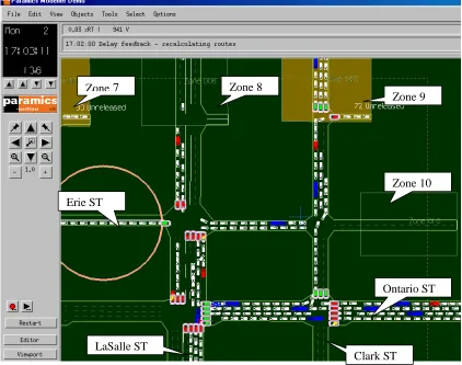
Figure 3.1 Gridlock cause with the Solver OD
Further probing of the results indicated that the statistical fitting method
generated unrealistic traffic demand in the Clark Street at Erie Street area (see
Figure 3.1). Field observations had shown that southbound Clark at Erie had a
left turn percentage of around 8%, which was about 100 vehicles turning left
during the subject time period. However, the solutions generated by statistical
fitting method had a much lower traffic demand from zone 9 to zone 10, which
was balanced by a greater demand from zone 9 to zones located west of LaSalle
and from those zones to zone 10. As a result, these solutions had put more Zone 9
Zone 10 Zone 8
Zone7
Clark ST
Ontario ST Erie ST
through vehicles on eastbound Erie Street at Clark and more right turns on SB
Clark Street at Ontario.
EB Erie Street is stop-controlled and has a small capacity. Also, the heavy usage
of the right-turn lane from SB Clark to WB Ontario caused spillback that further
aggravated the situation. It was observed that just about all gridlocks were
initiated at that location.
It is hypothesized that the statistical fitting method gives preference to long trips.
Obviously, with the same amount of adjustment, changing to longer trips would
enable faster fitting to the empirical data since longer trips would include more
links that can be adjusted at the same time.
As a result, shorter OD trips were decreased or even eliminated in the solution
process and longer OD trips were increased. This resulted in difficult turning
movements at some sensitive intersections, thus leading to a high risk of
breakdown on the whole network. To avoid this problem, turn movement volume
fitting error could be used as the objective function. However, these data are too
expensive to gather in the field, and it would explode the dimensions of the
optimization problem.
A modification of the statistical method was to constrain the true traffic demand
feasible OD pairs. The constrained solutions from different objective functions
were satisfactory in generating successful Paramics runs and yielded lower SSE
or SCSE. The results are shown in Table 3.4.
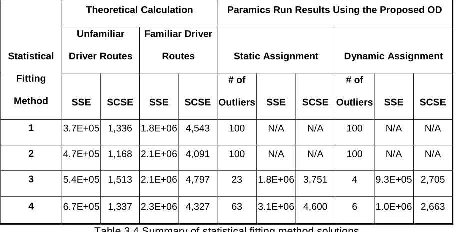
Table 3.4 Summary of statistical fitting method solutions
Note: fitting method 1 is calculated to minimize link volume SSE (sum square
error) by adjusting all feasible OD pairs, method 2 is calculated to minimize
SCSE (sum chi-square method) by adjusting all feasible OD pairs, method 3 is to
minimize SSE by keeping SB Clark OD pairs to be derived values from the
stochastic assignment method and adjusting other feasible OD pairs, and
method 4 is subject to the same conditions as method 3, but to minimize SCSE. Theoretical Calculation Paramics Run Results Using the Proposed OD
Unfamiliar
Driver Routes
Familiar Driver
Routes Static Assignment Dynamic Assignment Statistical
Fitting
Method SSE SCSE SSE SCSE
# of
Outliers SSE SCSE
# of
Outliers SSE SCSE
1 3.7E+05 1,336 1.8E+06 4,543 100 N/A N/A 100 N/A N/A
2 4.7E+05 1,168 2.1E+06 4,091 100 N/A N/A 100 N/A N/A
3 5.4E+05 1,513 2.1E+06 4,797 23 1.8E+06 3,751 4 9.3E+05 2,705
3.3 Stochastic Assignment Method
Approach
The stochastic assignment method is based on the entry volumes and turning
probabilities that were gathered in the field and used in CORSIM. It is assumed
that vehicle routing is based on a stochastic traffic assignment method, where
vehicles are assigned to downstream links stochastically, and independent of
their network origins.
Since vehicles between origin zone i and destination zone j are assigned to
downstream links according to prescribed turning probabilities, then, for a
particular route r containing
n
links (link 0 corresponds an entry link, link ncorresponds an exit link) with an entry volume of Er,
∏
= −=
n k k k r rij
E
P
od
1 , 1
Where
P
k−1,k denotes turning probability from link k-1 to link k.For one particular OD pair, vehicle demand would equal the aggregation of
vehicle trips traveling through all possible routes between the origin and the
The OD matrix solution could be solved pair-by-pair using the same method as
above.
Manual calculation or even computer programming for this method is laborious.
Therefore the solution could be achieved by simulating CORSIM.
A series of single-source CORSIM runs were carried out, each having a single
entry volume as traffic demand.
For each single-source run, the traffic volumes at all exit links were gathered as
the pair values for one corresponding row of the OD matrix. The solution OD
matrix was solved through running the single source network for each origin input
Figure 3.2 Single-source CORSIM network (WB Ontario)
To avoid extreme randomness, the median values from multiple CORSIM runs
were collected as the OD pair values. The derived solution is shown in Table 3.2:
FROM
\TO 1 2 3 4 5 6 7 8 9 10 11 12 13 14 15 16 17 18 19 20 21 22 23 * SUM 1 0 0 0 0 0 0 0 0 0 0 0 0 0 0 0 0 0 0 0 0 0 0 0 * 0 2 0 0 1 18 11 3 0 2 0 0 0 6 0 24 2 3 37 1 6 66 24 0 32 * 236 3 2 3 0 14 4 1 0 0 0 0 0 0 0 0 0 1 3 0 1 4 4 0 7 * 44 4 1 5 0 0 2 1 0 4 0 1 0 2 0 2 1 1 5 0 1 3 5 0 12 * 46 5 4 8 0 9 0 22 0 22 0 27 0 8 0 17 8 9 31 8 0 20 13 0 625 * 831 6 1 2 0 3 5 0 0 5 0 4 0 15 0 24 4 6 12 19 1 3 11 0 71 * 186 7 0 5 0 7 21 8 0 23 0 10 0 54 0 90 18 17 183 1 0 3 21 0 84 * 545 8 4 2 0 0 15 12 17 0 0 25 0 99 0 55 17 471 11 1 2 2 39 0 198 * 970 9 0 1 0 0 18 13 0 41 0 106 0 154 0 119 621 17 8 1 1 6 25 0 282 * 1413 10 0 0 0 0 0 0 0 0 0 0 0 0 0 0 0 0 0 0 0 0 0 0 0 * 0 11 0 2 0 4 56 44 1 136 0 15 0 31 0 38 102 79 29 1 2 2 11 0 1379 * 1932 12 0 0 0 0 0 0 0 0 0 0 0 0 0 0 0 0 0 0 0 0 0 0 0 * 0 13 1 12 2 8 93 31 1 137 0 10 0 33 0 57 176 56 51 9 10 24 383 0 169 * 1263 14 0 0 0 0 0 0 0 0 0 0 0 0 0 0 0 0 0 0 0 0 0 0 0 * 0 15 0 0 0 0 0 0 0 0 0 0 0 0 0 0 0 0 0 0 0 0 0 0 0 * 0 16 0 0 0 4 18 14 7 806 0 41 0 103 0 99 38 0 7 3 0 3 43 0 209 * 1395 17 0 0 0 0 0 0 0 0 0 0 0 0 0 0 0 0 0 0 0 0 0 0 0 * 0 18 0 1 0 1 17 110 0 10 0 10 0 23 0 51 10 16 49 0 1 2 33 0 80 * 414 19 0 38 1 15 448 13 1 16 0 4 0 51 0 64 18 15 61 10 0 124 86 0 610 * 1575 20 0 16 1 2 1 0 0 0 0 0 0 0 0 4 0 0 4 0 0 0 14 0 5 * 47 21 0 31 1 9 48 18 0 7 0 3 0 7 0 65 12 8 131 3 9 28 0 0 78 * 458 22 2 8 0 6 364 28 2 148 0 22 0 795 0 74 90 51 106 9 72 9 47 0 57 * 1890 23 0 0 0 0 0 0 0 0 0 0 0 0 0 0 0 0 0 0 0 0 0 0 0 * 0
* * * * * * * * * * * * * * * * * * * * * * * * * * SUM 15 134 6 100 1121 318 29 1357 0 278 0 1381 0 783 1117 750 728 66 106 299 759 0 3898 * 13245
The solution OD matrix was run in Paramics. The results were encouraging in
that a small number of gridlocks were generated and traffic volumes on most
links were close to the known link volumes.
3.4 Adopted OD Matrix after Manual Adjustment
Roundtrips in the Stochastic Assignment Method Solution
Further observations of Paramics running with the solution OD from the
stochastic assignment method showed that some inner links had lower traffic
than expected, whereas the boundary links had better fitting results to the known
This occurred because the stochastic assignment method could yield round trips
between OD pairs (See Figure 3.3). In flow-based simulation models, vehicles
could be assigned stochastically, so that some round trips would be generated in
a series of consecutive left turns or right turns; in the real world and in
route-based simulation models, vehicles would not enter the inside network and circle
around if they could go though boundary areas to reach their destinations directly.
Therefore these round trips should be transferred to other reasonable OD pairs.
OD Solution after Manual Adjustment
To zero out these round trips and keep the marginal values of rows and columns
fixed at the same time, a rectangular adjustment method was used.
For any OD pair (i, j) to be adjusted to 0, another corresponding OD pair (l, m) is
found. Assume the adjustment amount is A, the pairs (i, j) and (l, m) would be
decreased by A, and at the same timepairs (l, j) and (i, m) would be increased by
A.
Performing this adjustment requires network-specific knowledge in order to
decide which corresponding pairs to assign the adjusted traffic to. In this case, a
or about 5% of total network demand, were manually adjusted using this method.