Design Techniques for High Efficiency Highly Linear RF Power Amplifer

(1)

PREM SWAROOP, SHANTHA MURTHY. Design Techniques for High Efficiency Highly Linear RF Power Amplifier. (Under the direction of Dr. Kevin Gard).

Power consumption is a key parameter to be considered in designing wireless sys-tems, especially for cellular applications. Lower power consumption by designing

highly power efficient transceiver circuits is extremely desirable as it results in lower

battery size, higher talk time, lower heat generation and lower cost. Very high spectral efficiency is sought after in present day communication systems. In order to achieve

very high data rates, sophisticated non-constant envelope modulation schemes are

used. This places very stringent requirements on the transceiver design. One of the

key requirements is spectral linearity or purity, wherein the transmitter signal spec-trum has to be clean within the signal bandwidth and outside the signal bandwidth

as specified by FCC regulations for the wireless standard.

Output RF power amplifier (PA) consumes most of the power in a transmitter and is the key to high efficiency transmitter design. This research focuses on novel

techniques to maximize power efficiency of the RF power amplifier and at the same

time having high spectral linearity to meet FCC specifications. This research attempts to achieve the goal of high efficiency and high linearity by two different methods

-signal conditioning and smart circuit design.

A new crest factor reduction (CFR) technique to developed to reduce peak to average ratio (PAR) of high PAR signals. Trade-offs between the in-band and

out-of-band distortion is analyzed for maximum reduction in PAR of the signal.

A novel high efficiency linear transmitter architecture based on power quadrature modulation is proposed. High efficiency differential class D power supply modulator

is designed in Jazz 0.18 µm process.

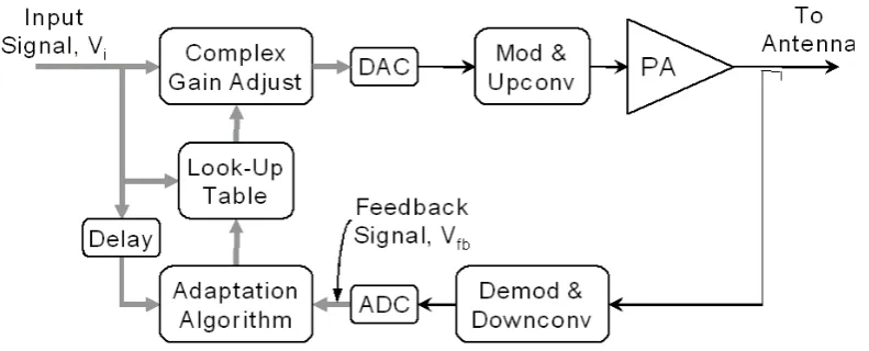
A lookup table based digital predistortion (DPD) engine is developed in

MAT-LAB to improve linearity performance in RF power amplifier. A DPD algorithm is demonstrated to improve the distortion performance of a Gallium Nitride RF PA at

(2)

by

Shantha Murthy Prem Swaroop

A dissertation submitted to the Graduate Faculty of North Carolina State University

in partial fullfillment of the requirements for the Degree of

Doctor of Philosophy

Electrical Engineering

Raleigh, North Carolina

2010

APPROVED BY:

Dr. Alex Huang Dr. Harvey Charlton

(3)

DEDICATION

To

(4)

BIOGRAPHY

Shantha Murthy Prem Swaroop was born and raised in Bangalore, India. He received

his B.Tech (Bachelors of Technology) degree in Electrical Engineering from Indian Institute of Technology, Madras in 2002. He worked as an IC design engineer in the

high resolution data converter group at Analog Devices in Bangalore from 2002 to

2004. He received Masters degree in English Literature from Karnataka State Open

University, Mysore in 2004.

He joined the department of Electrical and Computer Engineering at North

Car-olina State University in 2004 to pursue a Ph.D in the Radio Analysis and Design

group. His research interests include analog and RF integrated circuits for wireless and biomedical applications.

He is a student member of Institute of Electrical and Electronics Engineers (IEEE)

and Eta Kappa Nu (HKN). He was the Indian National Puzzle Champion in 2003 and has represented India in the 9th_{, 12}th_{, and 14}th _{World Puzzle Championships at}

Stamford, USA, Papendal, Netherlands and Eger, Hungary in 2000, 2003, and 2005

respectively. He is the recipient of Analog Devices Outstanding Student Design Award in 2006. He was one of the top 5 finalists in Semiconductor Research Consortium

(5)

ACKNOWLEDGMENTS

I would like to thank my parents for their undying support and encouragement

throughout my student life. It is their dreams that I am fulfilling with this PhD. I want to thank my wife and sweetheart Divya for her support, understanding

and standing by me through times - happy and tough, long distance and waiting

for weekends. I want to thank my Parents-in-law and Deepa for their unswerving

support throughout this time. I really appreciate their help and effort in making the long distance relationship work smoothly.

I have made some good friends during this time. Thanks to all who have made

a mark on me. I would like to thank two special friends Anand and Pochih, unique in their way, for their unconditional friendship. I really enjoyed all the coffee shop

hangouts, counselling sessions, question and answer bouts.

Special thanks to Two Cents of Hope and all its volunteers (each and everyone over the past 5 years) for making my life at NC State worthwhile and meaningful.

Thanks to Ravi Jenkal for all the lunches and interesting perspectives about life

and everything; Mithun for all the enjoyable racquetball, squash duels and the steam room outings!; My room mates for two years Akshay, Amar and Vineet for making

my start here a memorable one; Steve Lipa, Jonathan Wilkerson, Gautham

Krish-namurthy for help in the lab and perspectives about life in the ECE department; Elaine Hardin for being such a sweetie and making my life comparitively easier in the

bureaucratic-form-filling-make-your-life-miserable ECE department and its policies.

Thanks to Tony Montalvo of Analog Devices for the internships and being on my committee. Thanks to folks at Analog Devices, especially David Maclaurin for all

the fun times at AD and for giving me an insight into how lethal the combination of

super smartness and humility looks like.

Lastly, I would like to appreciate my Advisor Kevin Gard for his great insight, his cool attitude, his guidance and direction. It could have been a better ending, but I

(6)

(7)

LIST OF TABLES

Table 1.1 Summary of various wireless communication standards . . . 2

Table 2.1 Performance of various linearization techniques . . . 22

Table 2.2 Performance of different classes of linear amplifier . . . 22

Table 2.3 Comparison of power efficiencies for various design techniques . . . 32

Table 3.1 Noise Filtering due to Different Values of Weighting Factors . . . 40

Table 3.2 Forward Link WCDMA FCC Specifications . . . 41

Table 3.3 EVM due to different Clipping Levels and Weighting Factors . . . 46

Table 3.4 WLAN Spectral Requirements . . . 46

Table 3.5 EVM for Two Stage CFR . . . 47

Table 3.6 EVM for Three Stage CFR . . . 49

Table 4.1 Class-D Modulator Target Specifications . . . 60

Table 4.2 Class-D Modulator Top Level Pad Description . . . 74

(11)

Table 4.4 Reverse Link IS-95 FCC Specifications . . . 83

Table 4.5 Two-tone Signal Simulation Results . . . 84

Table 4.6 Two-tone Signal Simulation Results . . . 84

Table 4.7 Corner Simulation Results . . . 86

Table 4.8 Board Description . . . 88

Table 4.9 Decoupling Capacitor Bank . . . 89

Table 4.10 Output Filter Capacitor Bank . . . 89

Table 4.11 Sinusoidal Input Spur Suppression . . . 91

Table 4.12 Spectral Requirements for 900 MHz and 1800 MHz EDGE Handset signal . . . 91

(12)

LIST OF FIGURES

Figure 1.1 Generic Gain System . . . 3

Figure 1.2 Output spectrum of a non-linear system for a two-tone input . . . 4

Figure 2.1 Negative Feedback Block Diagram . . . 12

Figure 2.2 Cartesian Feedback Block Diagram . . . 15

Figure 2.3 Polar Feedback Block Diagram . . . 15

Figure 2.4 Feedforward System Block Diagram . . . 17

Figure 2.5 Predistortion Block Diagram . . . 19

Figure 2.6 Graphical Representation of Predistortion . . . 19

Figure 2.7 Envelope Elimination and Restoration Block Diagram . . . 24

Figure 2.8 Envelope Tracking Block Diagram . . . 27

Figure 2.9 Polar Modulation Block Diagram . . . 29

Figure 3.1 New CFR Technique Signal Flow Diagram . . . 35

Figure 3.2 Original and Clipped Signals . . . 36

Figure 3.3 Original and Clipped Signals and their corresponding spectrum . . . . 37

Figure 3.4 New CFR Technique Block Diagram . . . 38

Figure 3.5 Correlated and Uncorrelated Spectrum of a Clipped Signal . . . 39

Figure 3.6 WCDMA ACPR for various values of PAR andwO;wI = 1 . . . 42

Figure 3.7 WCDMA EVM for various values of PAR andwO;wI = 1 . . . 43

(13)

Figure 3.9 WCDMA EVM for various values of wO and wI; PAR= 5.7 dB . . . 44

Figure 3.10 WCDMA ACPR for various values of wO and wI; PAR= 7 dB . . . 45

Figure 3.11 WCDMA EVM for various values of wO and wI; PAR= 7 dB . . . 45

Figure 3.12 WLAN EVM for different values ofwI,wO . . . 47

Figure 3.13 Modified three stage CFR technique for WLAN signals . . . 48

Figure 3.14 Optimized three stage CFR WLAN Output Spectrum . . . 50

Figure 3.15 Optimized EVM for various PAR using CFR . . . 51

Figure 3.16 PA Output: ACPR for various values of wO and wI; PAR= 5.7 dB . 51 Figure 3.17 PA Output: EVM for various values of wO and wI; PAR= 5.7 dB . . 52

Figure 3.18 PA Output: ACPR for various values of wO and wI; PAR= 7 dB . . . 52

Figure 3.19 PA Output: EVM for various values of wO and wI; PAR= 7 dB . . . . 53

Figure 3.20 PA Output: ACPR and PAE with and without CFR+DPD . . . 53

Figure 3.21 PA Output: EVM with and without CFR+DPD . . . 54

Figure 4.1 Proposed Power Quadrature Modulator Architecture . . . 58

Figure 4.2 H-Bridge Class-D Modulator Block Diagram . . . 61

Figure 4.3 PWM Single-ended and Differential Spectra . . . 62

Figure 4.4 Comparator Circuit . . . 63

Figure 4.5 Dead-time Generation Circuit . . . 65

Figure 4.6 Outputs of Dead-time Generation Circuit . . . 66

Figure 4.7 Effect of Dead-time in the Power Stage . . . 67

Figure 4.8 Second Order Filter Magnitude Response . . . 71

(14)

Figure 4.10 Bonding Diagram on a 44 pin QFN package . . . 76

Figure 4.11 Simulation plots of PMOS and NMOS on-resistance for various Gate-Source voltages . . . 77

Figure 4.12 Simulation results of power losses for various power stage widths . . . 78

Figure 4.13 Simulated Power efficiency for various Power stage widths . . . 78

Figure 4.14 Simulated Modulator output power and power efficiency for various modulation indices . . . 79

Figure 4.15 Simulated IMD Vs Dead-time . . . 80

Figure 4.16 Simulated Power Efficiency Vs Dead-time . . . 80

Figure 4.17 Simulated Second Harmonic IMD Vs Switching frequency . . . 82

Figure 4.18 Simulated Power Efficiency Vs Switching frequency . . . 82

Figure 4.19 Two-Tone Differential Output spectrum . . . 84

Figure 4.20 Two-Tone Single Ended Output spectrum . . . 85

Figure 4.21 IS-95 Differential Output spectrum. . . 85

Figure 4.22 IS-95 Single Ended Output spectrum . . . 86

Figure 4.23 Two Layer Board Design . . . 87

Figure 4.24 Differential and Single Ended Modulator Output Spectrum for 200 KHz Sinusoidal Input Signal . . . 90

Figure 4.25 Nearband Differential and Single Ended Spectrum for EDGE Input Signal . . . 92

Figure 4.26 Wideband Differential and Single Ended Spectrum for EDGE Input Signal . . . 93

Figure 4.27 Measured, Simulated and Modelled modulator power efficiency . . . 94

Figure 5.1 Digital Predistortion Block Diagram . . . 96

(15)

Figure 5.3 Post DPD ACLR and PAE Vs Gate Bias Voltage . . . 99

Figure 5.4 Pre and Post DPD Output Spectra . . . 99

Figure 5.5 Post DPD + CFR ACLR and PAE Vs Output Power . . . 100

Figure 5.6 EVM Vs PAR . . . 100

Figure 6.1 HELT Characterization Block Diagram . . . 104

Figure A-1 Comparator Schematic . . . 112

Figure A-2 Bias Generator Schematic . . . 113

Figure A-3 Dead-time Generation Schematic . . . 113

Figure A-4 Dead-time Fine Delay Schematic . . . 114

Figure A-5 Dead-time Coarse Delay Schematic . . . 114

Figure A-6 P-Driver Level Shifter Schematic . . . 115

Figure A-7 N-Driver Level Shifter Schematic . . . 115

Figure A-1 Class-D Modulator Top Level Layout . . . 116

Figure A-2 Comparator Layout . . . 117

Figure A-3 Bias Generator Layout . . . 118

Figure A-4 ESD Power Supply Clamp Layout . . . 119

Figure A-5 I/O connecting ESD Diodes Layout . . . 120

Figure A-6 Dead-time generation Circuit Layout . . . 121

Figure A-7 P-Driver Level Shifter Layout . . . 122

(16)

Chapter 1 INTRODUCTION

1.1 Background

In first generation (1G) wireless systems like NMT (Nordic Mobile Telephone) and

AMPS (Advanced Mobile Phone System), the throughput rates were pretty moderate

(few kbps). Constant envelope modulation schemes were used to achieve the necessary data rates. In GSM (Global System for Mobile Communications), a second

gener-ation (2G) system, GMSK (Gaussian Minimum Shift Keying), a constant envelope

modulation scheme is used to obtain data rate of about 270 Kbps. EDGE (Enhanced

Data Rate for GSM Evolution) provides three times the data rate as GSM by addition of amplitude modulation along with phase modulation, however utilizing the same

bandwidth. IS-95 (Interim Standard), a 2G standard pioneered by Qualcomm, and

branded as cdmaOne, uses CDMA (Code Division Multiple Access) as opposed to TDMA (Time Division Multiple Access) used by GSM or Frequency division

multi-plexing used by 1G cellular systems. Here QPSK (Quadrature Phase Shift Keying),

a non-constant envelope scheme is used to obtain higher throughput rate of 1.2288 Mbps. 3G systems like WCDMA (Wideband Code Division Multiple Access) make

use of non constant envelope schemes to achieve higher data rates. WCDMA has a

(17)

data rates up to 54 Mbps. WiMAX (Worldwide Interoperability for Microwave Ac-cess) uses OFDM (802.16d) and SOFDMA (Scalable Orthogonal Frequency Division

Multiple Access) (802.16e) and can achieve data rates as high as 70 Mbps. Summary

of various wireless communication standards is presented in table 1.1 [3].

Table 1.1: Summary of various wireless communication standards

Spectral efficiency is an extremely important parameter in present day communi-cation systems. In order to achieve very high data rates, sophisticated modulation

schemes are used, which use non-constant envelope schemes. Very stringent

require-ments are put on the transceiver design. One of the key requirerequire-ments is spectral linearity or purity, wherein the transmitter signal spectrum has to be clean within

the signal bandwidth and outside the signal bandwidth as specified by FCC

regula-tions for the wireless standard.

Power consumption is a key parameter to be considered in wireless systems, espe-cially for cellular applications. Lower power consumption by designing highly power

efficient transceiver circuits is extremely desirable as it results in lower battery size,

(18)

Concepts of Linearity and Power efficiency are explained in detail from the trans-mitter point of view in the following subsections.

1.2 Linearity

A system is called linear if the output varies in direct proportion to the input.

Conversely, a system is called non-linear if the output is a non-linear function of the

input.

x

G(x)

y

Figure 1.1: Generic Gain System

Consider the system shown in fig. 1.1. As per eqn. 1.1, the output of the system y

is given in terms of the input x and system gain G. The system is linear if the system

gain is independent of the input x.

y = G(x) x (1.1)

Polynomial modelling can be used to model the non-linearity of a system as shown

in eqn. 1.2.

y = g0+g1 x+g2 x2+g3 x3+...+gn xn (1.2)

Hereg0−gn are constant complex coefficients obtained from narrowband

(19)

A two-tone analysis helps in understanding the different spectral components gen-erated due to non-linearities in the system. Consider a two-tone input signal as given

by eqn. 1.3

x = A Cos(w1 t) +A Cos(w2 t) (1.3)

Herew1 and w2 are the two input frequencies and A is the amplitude of the input

tones.

DC FIRST

HARMONIC

SECOND HARMONIC

THIRD HARMONIC DC w₂- w₁ 2w₂- w₁ w₁ w₂ w- 2 w₂ ₁ 2w₁ w₂+ w₁ 2w₂ 3w₁w+ 2w₂ ₁2w₂ + w₁3w₂

Figure 1.2: Output spectrum of a non-linear system for a two-tone input

Limiting the polynomial expansion to third order, the output spectrum obtained is shown in fig. 1.2. The output spectrum contains components around DC, first,

second and third harmonics of the input frequencies. There are frequency components

at DC and the envelope frequency (w2−w1) due to second order non-linearities in the

system. The components around the first harmonic are atw1andw2due to first order

signals and mixing products due to third order distortion. There are also components

at 2w1−w2 and 2w2−w1 due to third order non-linearities in the system. There are

spectral components around second and third harmonics of the input frequency due

to second and third order non-linearities in the system.

(20)

cannot be removed as they are very close to the signal band. Substituting eqn. 1.3 in eqn. 1.2, the amplitude of first harmonic components (Y1) and the IM3 components

(Y3) are given by eqns. 1.4 and 1.5

Y1 = g1+

9 4 g3 A

3 _(1.4)

Y3 =

3 4 g3 A

3

(1.5)

The second term in eqn. 1.4 corresponds to gain compression/expansion and Y3

in eqn. 1.5 corresponds to intermodulation distortion.

Writing g3 as a complex number

g3 = g3R+j g3I (1.6)

and substituting eqn. 1.6 in 1.4

Y1 = Y1AM P tan−1(φ1) (1.7)

Where,

Y1AM P = g1 A s

1 + 9 4

g3R A2

g1 2

+

g3I A2

g1 2

(1.8)

φ1 =

1 g3R

g3I

+ ₉ g1

4 g3I A2

(1.9)

Y1AM P is a measure of AM-AM distortion and φ1 is a measure of AM-PM

(21)

Note: Expressing a signal as a polynomial expansion is a narrow band represen-tation. It is just a qualitative measure of linearity of a signal and cannot be extended

to wide-band signals.

In digital communication systems, BER (Bit Error Rate) is a system performance

metric that quantifies the reliability of the entire system, defined by eqn. 1.10.

BER = Number of errors

Total number of bits transmitted (1.10)

SNR (Signal to Noise Ratio), EVM (Error Vector Magnitude) and ρ (waveform quality factor) are system performance metrics used to measure distortion in the

channel. SNR is the ratio of the signal power to the total noise power in the channel. EVM is a measure of the departure of signal constellation from its ideal reference

because of nonlinearity. ρis a measure of the correlation between a scaled version of the input and the total in-channel output waveforms. The relationship between these metrics has been established in [1].

EV M =

r

1

SN R (1.11)

ρ = SN R

SN R+ 1 (1.12)

Further, the in-band distortion contains distortion components that are correlated

and uncorrelated to the input signal. The correlated component results in gain

com-pression/expansion, whereas the uncorrelated component represents the in-band noise floor. The ratio of the desired output signal power to the power of the uncorrelated

distortion component is used to calculate SNR, EVM and ρ. Correlation techniques are used in [2] to separate the correlated and uncorrelated distortion components. An analytical evaluation of BER using the SNR obtained from the output spectrum is

verified using simulations.

(22)

distortion results in the degradation of SNR and ultimately BER itself. Out-of-band distortion results in degradation of SNR of adjacent channels. ACPR (Adjacent

Channel Power Ratio) is a measure of out-of-band distortion, which is the ratio of

the channel signal power to the noise added in the adjacent channel.

Receiver noise is a critical specification in transmitter design. It determines how

much noise is allowed at receiver frequencies and is measured in dBc/Hz. Noise at

the receiver limits receiver sensitivity. Thermal noise in the resistance of the signal

source is the fundamental limit on achievable signal sensitivity. Noise floor Power (NFP) is given by

N F P = k T B (1.13)

Here,

K is Boltzmann Constant = 1.38 X 10−23 J/K T is the absolute temperature in ◦K

B is the noise bandwidth in Hz

Noise floor power at 290 K (the standard for definition of noise floor) using eqn. 1.13 is equal to -174 dBm/Hz.

Other noise sources in the transmitter affecting the receiver sensitivity are phase

noise from the local oscillator and wideband out-of-band distortion due to the non-linearity of the RF PA.

1.3 Peak to Average Ratio

PAR (Peak-to-Average Ratio) is a method of defining the statistics of a modulated signal in terms of Peak power and Average power. PAR is defined as the ratio of Peak

power of the signal to the average power of the signal. It is usually expressed in dB.

Qualitatively PAR is a measure of the dynamic range of the signal. Higher the PAR,

(23)

given in eqn. 1.14. Here E is the statistical mean of the signal.

P AR = 10 log

max(|x|)2

E(|x|)2

(1.14)

Other measures like CF (Crest Factor) are used to determine the statistical nature

of the modulated signal. CF is the ratio of the peak amplitude to the rms amplitude

of the signal.

1.4 Efficiency

Spectral purity and spectral efficiency are two very important parameters involved

in the design of a cellular data transmission system. Spectral purity translates to lin-earity and spectral efficiency translates to throughput rate. One other very important

parameter in the design of cellular networks is the power consumption.

Power consumption is a very important parameter both in Base station as well as Handset designs. Handsets, since running on batteries, rely heavily on lower power

consumption to maximize talk-time or on-time. Base stations on the other hand would

desire lower consumption keeping in mind the thermal effects caused by temperature increase due to heavy power consumption. A very big portion of the power consumed

in a transmitter goes into the PA. So, the designed PA has to be power efficient.

Power efficiency and Power Added Efficiency (PAE) are two important measures of efficiency of a system.

Power efficiency is defined as

η = POU T PDC

(1.15)

Where POU T is the Output RF power and PDC is the power consumed from DC

source.

(24)

P AE = POU T −PIN PDC

(1.16)

1.5 Problem Statement

Present day 2.5 G and 3 G communication systems use sophisticated non-constant

envelope schemes like WCDMA and OFDM to achieve high spectral efficiency. These modulation schemes have very high PAR, often execeeding 10 dB. The output of

the transmitter needs to be highly linear over a wide dynamic range when using

linear mode RF power amplifiers (PA) like class A, B, AB and C amplifiers, since the information is contained in amplitude as well as phase of the signal.

It is clear that the IM3, IM5 and other higher order distortion components increase

by 3 dB, 5 dB and so on for every dB increase in the output power, thereby degrading the linearity as the output power increases. Hence, the amplifier average output power

needs to be backed-off from the 1 dB gain compression point by at least the PAR of

the input signal. The PA has to be designed for the peak power but will be operating mostly around the average power level.

From eqn. 1.16, it is also clear that higher the RF power delivered to the load,

higher is the PAE. Also, beyond the 1-dB compression point, the output power de-livered remains constant, not changing with increase in input power. This decreases

the PAE of the PA. So, in order to obtain highest possible efficiency, it is desired

to drive the PA as hard as possible just close to its 1-dB compression point but not

going beyond the compression point. Hence, working in a backed-off mode results in really poor power efficiency of the PA and the transmitter.

This implies that there is a direct trade-off between the linearity and power

effi-ciency for spectrally efficient modulation schemes. One seems to be achieved at the expense of the other. Hence, it is imperative to have external linearization schemes

to improve the linearity and power efficiency enhancement schemes to improve the

(25)

The underlying problem is to design systems with improved linearity and at the same time improving or at least not degrading the system power efficiency, knowing

that an inverse relationship exists between the two parameters.

1.6 Overview of Thesis

The focus of this research is to design high efficiency, highly linear CMOS RF amplifiers for 2.5 G and 3 G communication systems using spectrally efficient

mod-ulation schemes. This research attempts to achieve the goal of high efficiency and

high linearity by two different methods - signal conditioning and smart circuit design. Chapter 2 describes the various linearization and efficiency improvement techniques

available in literature. A new CFR (Crest Factor Reduction) technique to reduce

the PAR of high PAR signals is presented in chapter 3. Reduction of PAR results in increased power efficiency of the system. Trade-off between the in-band and

out-of-band distortion is presented for the maximum reduction in PAR of the signal. The

proposed CFR technique is demonstrated using WCDMA and WLAN signals on a Gallium Nitride (GaN) RF Power Amplifier (PA). A new HELT (High Efficiency

Lin-ear Transmitter) architecture using CMOS switch-mode RF amplifiers and class D

amplitude modulators is proposed in chapter 4. Detailed discussion of the motivation

behind the proposed technique, theory of operation, design of the class D modulator and measurement results are presented in this chapter. Chapter 5 describes a LUT

(Look Up Table) based DPD (Digital Predistortion) technique used to improve the

linearity of the RF PA. A DPD algorithm is demonstrated to improve the distortion performance of a GaN (Gallium Nitride) PA at a particular output power level. DPD

in conjunction with CFR can be used to improve the overall linearity and PAE of the

(26)

Chapter 2 Linearization and Efficiency

Improvement Techniques

2.1 Linearization Techniques

This section describes some of the popular linearization techniques available in

literature. Detailed analysis of various linearization techniques is done in [4], [5], and [6].

Any system can be linearized by one or more of the following methods.

1. Fabrication of more linear devices.

2. Limiting operation of devices to most linear region of operation.

3. Deliberate addition of distortion somewhere in the system to compensate for non-linearities created by the devices in the system.

Working within the realms of circuit design techniques, only the second and mainly

(27)

2.1.1 Back-off

The simplest means of achieving a good linearity is to back-off from the 1-db

compression point by at least the PAR of the modulation signal. This may give better linearity performance but heavily at the cost of efficiency. This technique has

limited scope of use.

2.1.2 Feedback

Feedback is probably the simplest and most intuitive linearization technique. The basic essence of feedback is to reduce the error or distortion in the output signal by

feeding a portion of the output signal back to the input. The feedback applied can

be of two types-positive and negative. Positive feedback increases the error, whereas,

on the other hand, negative feedback reduces the error in the system.

x e G y

f v

Σ

+

-Figure 2.1: Negative Feedback Block Diagram

Consider the block diagram shown in fig. 2.1. Prior to feedback, the output signal in terms of the input signal is given by eqn. 2.1.

(28)

Here G is the non-linear gain of the system. On applying negative feedback with feedback factor f,

y = G e (2.2)

Here, e is the error signal fed to the system given by eqn 2.3

e = x−f y (2.3)

Simplifying,

y = G

1 +G f x (2.4)

For a high value of the loop gain G f, i.e, G f 1, eqn. 2.4 reduces to

y = 1

f x (2.5)

The feedback is done usually through a linear element and hence the feedback

factor f is highly linear. So from the above equation, the output signal y is dependent on the input signal x and the linear parameter f. It is independent of the system

non-linear gain G. Hence the output signal is a linear amplified version of the input

signal.

What essentially happens is that the input signal to the system is a very small

signal e of value ₁₊_{G f}1 x. Since the input seen is a small signal, the output is naturally a linear version of the input signal. Another way of looking at it is that the input e

to the system is predistorted automatically by the feedback in such a way that the output is linear. It is to be noted that the feedback, though linearizes the output

signal, reduces the gain of the system. The gain is reduced from G to _f1 by a factor of G f, which is the loop gain of the system.

One critical aspect of any feedback system is the loop stability. It is to be ensured

that the feedback loop is stable under all conditions as stated by the Nyquist stability

(29)

The input, output and feedback signals in the system can be signals of any type-voltage, current, phase, frequency, etc. The main system is an active system, whereas,

the feedback system is usually a linear passive element. The feedback can be of two

types - series and shunt feedback.

Feedback for RF systems RF itself. Feedback at RF This puts in a huge bandwidth

requirement on the system. An alternative to this is to down-convert the output RF

signal to baseband and provide feedback to the input baseband signal. Feedback can

also be provided at IF.

Applying feedback for RF systems, it is very important to match the delays for

the forward path and the feedback path. Delay mismatches reduce the effectiveness

of feedback. It may also lead to instability.

Based on the choice of coordinate system used to fully describe the modulation,

baseband feedback can be of two types, namely cartesian feedback and polar feedback.

If the complex baseband input signal is represented in terms of cartesian or I-Q format as in eqn. 2.6, then it is termed as cartesian feedback. The RF output is given in

eqn. 2.7 in terms of RF carrier w0. Simplified block diagram of cartesian feedback is

shown in fig. 2.2.

x(t) = I(t) +j Q(t) (2.6)

y(t) = I(t)Cos(w0 t) +Q(t) Sin(w0 t) (2.7)

Polar feedback makes use of polar representation of the complex baseband signal

as shown in eqn. 2.8. The RF output is shown in eqn. 2.9. Simplified block diagram

of polar feedback is shown in fig. 2.3. A PLL (Phase Locked Loop), a negative feedback control system is used to control the phase of the signal and frequency of

operation. Following down-conversion of the output signal, the amplitude is fed back

(30)

LO (w ) DOWN CONVERTER CONVERTER RF PA I Q y o

Σ

+

-Figure 2.2: Cartesian Feedback Block Diagram

RF OUTPUT AMPL MOD PHASE MOD SWITCH-MODE RF PA SWITCH-MODE/LINEAR ENVELOPE AMPLIFIER PHASE MAGNITUDE Rectangular To Polar I Q A Φ PLL VCO DOWN CONVERTER

Figure 2.3: Polar Feedback Block Diagram

(31)

y(t) = A(t) Sin(w0 t+φ(t)) (2.9)

Both types of feedback employ two feedback control loops. Polar feedback uses

one loop for the amplitude and one for the phase, whereas cartesian feedback uses two identical loops.

Ideally, a Cartesian feedback system functions as two identical, decoupled feedback

loops: one for the I component, and one for the Q component. However, in practice, due to delay through the RF PA, phase shifts of the RF carrier due to the reactive

load of the antenna, and mismatched interconnect lengths between the LO (local

oscillator) and the I-Q mixers result in phase misalignment and hence coupling of the I-Q loops. As a result, the stability of the feedback loops is greatly compromised.

A detailed analysis of phase misalignment in cartesian feedback and robust design

techniques to overcome this problem is presented in [7].

Similar problem exists in polar feedback. Here the problem is more severe as there are two different kinds of loops in polar feedback as compared to cartesian feedback,

where two identical loops are used. The phase and amplitude bandwidths are many

times higher than the baseband I-Q modulation bandwidth. Designing stable feedback loops for such high bandwidths is very challenging. The phase feedback loop is most

difficult to design as its spectrum extends all the way to infinity. Compromising on

the bandwidth results in severe spectral degradation, which is not acceptable to the present day wireless standards.

2.1.3 Feedforward

Feedforward linearization is similar to feedback linearization except that the

cor-rection is applied at the output of the system rather than the input of the system as in feedback. A simplified block diagram of feedforward linearization technique is

shown in fig. 2.4. The output v of the main non-linear RF PA A1 is given by eqn.

2.10. Here G1 is the linear gain of the amplifier and G(x) is the input dependent

(32)

G(x)

1/G

1 x

y

e

v

Figure 2.4: Feedforward System Block Diagram

v = G1 x+G(x) (2.10)

This output is fed to an attenuator having an attenuation factor G1 equal to the

linear gain of the main RF amplifier. Error signal e given by eqn. 2.11 is obtained

by subtracting the attenuated signal by the input to the RF PA.

e = v

G1

−x (2.11)

Substituting eqn. 2.10 in eqn. 2.11,

e = G(x)

G1

(2.12)

The error signal is amplified by a similar RF PA A2. Since, the signal level is

low, the output of this amplifier is fairly linear. Output of A1 is subtracted from the

(33)

y = v−G1 e (2.13)

Substituting eqns. 2.12 and 2.10 in eqn. 2.13,

y = G1 x (2.14)

We see from eqn. 2.14 that the output is linearly amplified version of the input. Feedforward linearization offers the benefits of feedback linearization without the

disadvantages of instability and bandwidth limitations.

Some of the disadvantages and challenges of feedforward linearization are

• An extra PA is required to amplify the error signal.

• The distortion performance of the additional PA places an upper limit on the

distortion correction offered by this technique.

• Accurate gain and phase tracking is required by the various elements in the

system.

• The tracking needs to be maintained over the modulation bandwidth of the

input signal, which can be as high as 10s of MHz depending on the modulation

scheme.

• Tracking also needs to be maintained over temperature and time.

2.1.4 Predistortion

Predistortion is a linearization technique which involves creation of distortion characteristic which is complementary to the RF PA distortion characteristic so that

the cascaded system is independent of distortion. Simplified block diagram of a

(34)

x

F(x)

v

G(v)

y

Predistortion

Function

Non-Linear

Amplifier

Figure 2.5: Predistortion Block Diagram

x F(x)

v G(v)

x y

Figure 2.6: Graphical Representation of Predistortion

linear function of the input x. A graphical representation of predistortion is shown

in fig. 2.6. An analytical expression for F is given through eqns. 2.15-2.19.

v = F(x) (2.15)

y = G(v) (2.16)

y = G(F(x)) (2.17)

The predistortion function F is chosen such that

G(F(x)) = C x (2.18)

Here C is a complex constant. Hence,

F(x) = G−1 (C x) (2.19)

(35)

And,

y = C x (2.21)

Based on the frequency at which the predistortion function operates, the

lineariza-tion technique is classified as RF, IF, or baseband predistorlineariza-tion. Various implemen-tations of these predistortion techniques are presented in [4].

The advantages of RF/IF predistortion techniques are

• Unconditionally stable. Predistortion technique is essentially open loop.

• Easy to implement. Lesser number of components required.

• Easy to use at high frequencies.

• Very high linearization bandwidth.

Some of the disadvantages are

• Modest linearity improvement compared to other techniques such as feedforward

or cartesian feedback.

• Difficult to compensate for higher order distortion terms.

• Optimum performance only at one power level.

With vast improvement in DSPs (Digital Signal Processor), Baseband

predistor-tion has become very attractive. Gain and phase weighting coefficients of the

predis-tortion function are stored in a DSP at baseband before upconversion to RF. Since, the predistortion function is in the digital domain, this technique is called DPD

(Dig-ital predistortion). The DSP coefficients can be constantly updated using feedback

from the output signal through downconversion to baseband. This technique is called Adaptive DPD.

DPD can compensate for higher order distortion terms and can give linearity

(36)

• Sampling rate must be several times the modulation bandwidth of the signal.

• Very high DSP speeds and hence high power consumption.

• The coefficients take several iterations to converge to proper values. This poses

a challenge for real time operation.

• Handling memory effects.

Memory effect is a phenomenon in which the output signal is not only a function of

the instantaneous input signal, but also a function of previous input values. Changes in amplitude and phase of distortion components are caused by changes in

instanta-neous bandwidth or modulating frequency of the input signal. The distinction from

non-linearity is that non-linearity generates new spectral components, whereas mem-ory effects shape the existing spectral components. It is to be noted that memmem-ory

effects have very high time constants.

A detailed analysis of memory effect and its various causes is done in [8]. Memory effect has been characterized and quantified in [9], [10], and [11]. A hybrid

predistor-tion correcpredistor-tion scheme is proposed in [12] in which adaptive DPD is used to correct

for wideband errors and an analog predistortion loop is used to compensate for the long time constant memory effects.

Chapter 5 covers in detail an adadptive DPD algorithm used to linearize GaN

PAs used for base-station purposes.

2.1.5 Summary

Table 2.1 summarizes the performance of various linearization techniques [13].

Adaptive DPD seems most favourable technique for our purposes as it provides rea-sonable linearity improvement at low cost for high modulation bandwidth wireless

(37)

Table 2.1: Performance of various linearization techniques

Linearization Correction capability Correction Bandwidth Relative

Technique (dB) (MHz) Cost

Feedback 10-20 <5 Medium

Feedforward 25-35 >100 High

RF/IF PD 5-10 > 25 Low

Adaptive DPD 10-20 > 50 Medium

2.2 Efficiency Enhancement Techniques

2.2.1 Types of Amplifiers

RF PAs are broadly classified into two categories, namely linear amplifiers and

switch-mode amplifiers. If the PA devices operate in the linear amplifying region,

then they are called linear amplifiers. If the devices operate as a switch, switching between the two power supply rails then they are termed switch-mode amplifiers.

Linear Amplifiers

Linear amplifiers are further classified into different classes - A, B, AB and C

based on the time of conduction of current, the operating bias point, or alternatively,

the conduction angle in the PA devices. Performance of different classes of linear

amplifier is presented in table 2.2. A detailed description of each of the PAs and efficiency calculations are present in [4] and [5].

Table 2.2: Performance of different classes of linear amplifier Class Time of conduction Maximum Theoretical Distortion

per cycle (%) Efficiency (%)

A 100 50 Lowest

B 50 78.5 High

AB 50-100 50-78.5 Medium

C <50 >78.5 Highest

(38)

It is to be noted that the efficiency numbers are obtained at peak output power level and for a constant amplitude sinusoidal waveforms. The efficiency numbers further

drop down at lower output power levels and high PAR input signals.

From the above observations, it can be concluded that linear amplifiers are not suitable for design of highly efficient PAs. Doherty PA is a technique proposed to

obtain high efficiency for high PAR signals [4], [5], [6]. However the efficiency cannot

go beyond the maximum theoretical efficiency given in table 2.2.

Switch-mode Amplifiers

Switch-mode PAs are amplifiers in which the power devices are used as switches:

They are either completely turned on or off. Theoretically these PAs have 100 % power efficiency as there is no current-voltage overlap. This means that when there

is current flow in the device, there is no voltage across it and similarly, when there

is a voltage across it, there is no current flow in the device. Switch mode PAs are classified in variety of classes such as D, E, F,F−1_{, S, and T. The classification is based}

on architectural differences due to various factors such as frequency of operation,

accounting of circuit imperfections, and filtering of higher order harmonics of the signal frequency.

Switch-mode PAs can be used with constant envelope schemes as the devices need

to be completely turned on or off. They cannot operate in the linear amplifying region. Hence, they are not suitable for non-constant envelope schemes. Also, the

distortion performance of switch mode PAs is poorer compared to linear amplifiers.

The following subsections describe efficiency enhancement schemes used for non-constant envelope schemes.

2.2.2 Envelope Elimination and Restoration

EER (Envelope elimination and restoration) is a technique proposed by Kahn [14] that provides high power efficiency when using non-constant envelope schemes when

(39)

A conceptual block diagram of an EER system is shown in fig. 2.7. As the name Envelope Elimination and Restoration suggests, the envelope of the signal is first

“eliminated” by a limiter to generate a constant amplitude phase signal.

Simultane-ously, the magnitude information is extracted by an envelope detector. The phase information is amplified using a non-linear switch-mode RF amplifier. The

magni-tude is amplified separately by an envelope amplifier which can be either linear or

switch-mode type. The amplified magnitude and phase signals are then recombined

to “restore” the desired RF output signal. The amplitude and phase signals can be easily recombined if the amplified magnitude signal directly modulates the power

supply of the switch-mode RF PA.

RF INPUT

RF OUTPUT ENVELOPE

DETECTOR

LIMITER

SWITCH-MODE RF PA SWITCH-MODE/LINEAR

ENVELOPE AMPLIFIER

PHASE MAGNITUDE

Figure 2.7: Envelope Elimination and Restoration Block Diagram

The greatest advantage of this architecture is that a switch-mode RF PA can be used to provide maximum power efficiency using non-constant envelope input signal.

The overall system efficiency η is given by eqn. 2.22. Here ηRF and ηEN V are the

(40)

η = ηRF ∗ηEN V (2.22)

The linearity of an EER transmitter depends primarily on parameters such as

bandwidth of the envelope amplifier that modulates the power supply of the RF PA and the delay mismatch between the magnitude and phase signals when they are

recombined at the RF PA. Linearity performance does not depend on the linearity

of the RF PA itself. the effects of delay mismatch and finite envelope bandwidth are shown through analysis and measurements in [15]. Intermodulation distortion due to

delay mismatch for a two tone input is shown to be

IM D ≈ 2π B_RF2 ∆τ2 (2.23)

Here BRF is the bandwidth of the RF signal and ∆τ is the delay mismatch.

A feedback path from the RF output to the input of the envelope amplifier ensures amplitude tracking between RF input and output waveforms. The feedback loop

reduces non-linearities due to delay mismatch between phase and envelope paths. It

also reduces non-linearities introduced by the switch-mode amplifier when it deviates from its ideal behaviour. [16] uses a feedback loop to the envelope path followed by

a Σ−∆ class-D switching power supply modulator. [17] uses a class S modulator

having a dual feedback loop structure: One from the RF output to the envelope input

and the other internally within the envelope modulator. The second feedback loop helps in reducing non-linearities in the envelope path due to the envelope detector.

A Wideband EER system using a linear opamp and a buck converter is presented in

[18].

Some of the practical issues with EER architecture are discussed in the subsection

below.

Practical Issues

(41)

can be expressed in terms of cartesian coordinates I(t) and Q(t) or in terms of polar coordinates A(t) and φ (t) shown in eqns. 2.6 and 2.8 respectively. The envelope and phase signals are expressed in terms of the baseband quadrature signals as shown

below

A(t) = pI(t)2₊_Q(t)2 _(2.24)

φ(t) = tan−1

Q(t) I(t)

(2.25)

The envelope signal is a non linear function of the baseband I-Q signals. Hence,

the bandwidth of the envelope signal is much higher than that of the I and Q signals. Hence, the envelope modulator has to be designed for much higher bandwidth than

the baseband bandwidth. Design of the envelope modulator becomes very challenging

for high modulation bandwidth input signals such as WCDMA and WiMax. The envelope path must have bandwidth in several 10s of MHz range.

The phase signal bandwidth is many times the baseband signal bandwidth. Hence

the RF PA must have a much higher bandwidth. This calls for higher precision in alignment of the envelope and phase signals as per eqn. 2.24.

It is also very difficult to design limiters with very high peak to minimum signal

ratio. Designing envelope detector can be challenging in CMOS technology due to

the lack of ideal diode operating at RF frequencies.

Use of linear envelope amplifiers for power supply modulation, makes the system

power inefficient. Use of switch-mode power supply modulation requires a reference

clock whose frequency is several times that of the envelope signal bandwidth. Higher the switching reference frequency, higher are the switching losses in the modulator

and hence, lower is the power efficiency. Also this implies higher envelope modulator

bandwidth, which makes the design very challenging.

The output of the power supply modulator requires a low pass filter to filter out the

clock frequency, its harmonics and IMD products of the envelope signal frequencies

(42)

MHz range implies the usage of bulky discrete L-C components. This is extremely undesirable for mobile applications which is heading towards single chip solution.

Suppression of clock spurs to the desired FCC levels is a considerable challenge in

this technique.

2.2.3 Envelope Tracking

ET (Envelope Tracking) is a technique whose architecture is very similar to EER.

Conceptual block diagram of ET system is shown in fig. 2.8. The only difference is that ET uses the RF input directly to the PA instead of the phase signal and makes

use of a linear RF PA instead of a switch-mode PA.

RF INPUT

RF OUTPUT ENVELOPE

DETECTOR

LINEAR RF PA SWITCH-MODE/LINEAR

ENVELOPE AMPLIFIER

MAGNITUDE

Figure 2.8: Envelope Tracking Block Diagram

A mathematical model for time alignment requirement is proposed in [19]. High efficiency ET systems for different wireless applications are proposed in [20], [21].

The advantages of ET over EER are as follows:

• Bandwidth of the RF input signal is lesser than that of the phase signal. Hence,

(43)

• Modest time alignment required when compared to precise time alignment

re-quired in case of EER.

• Envelope path bandwidth is lesser than that of EER since amplitude

informa-tion is present in the RF input signal. However, the bandwidth is greater than baseband I-Q bandwidth.

ET has the same challenges as EER in terms of suppression of clock spurs at clock

harmonics and IMD products of clock and envelope signal frequencies. The problem of envelope bandwidth vs power efficiency due to the choice of switching frequency

still exists. However the case is better when compared to EER.

Linearization schemes such as DPD can be used to improve in-band and near-band out-of-band distortion. However these cannot mitigate far away clock spurs.

A hybrid EER technique is proposed in [18], [22] to utilize the high efficiency

operation of EER and at the same time obtain the relaxed time alignment benefit of

ET. In this technique, the PA input signal is still the modulated RF signal. However, the RF PA is designed to operate in switch-mode for high output power levels and in

linear mode for lower output power levels.

The principle behind using this hybrid technique is as follows. A large portion of the energy of the non-linear envelope signal is concentrated from DC to several

KHz (85 % for OFDM) and almost all the energy (99 %) is concentrated below the

modulation bandwidth. This implies that a “split-band” envelope amplifier composed of a wideband but rather low efficiency linear stage and a high-efficiency narrowband

switch stage can achieve a high efficiency over a wide bandwidth. The overall average

efficiency η is a combination of the linear and switch-mode stage efficiencies namely ηLIN and ηSW respectively, given by eqn. 2.26. Here α is the power ratio given by

the ratio of the signal power from the switch stage to the total signal power.

η = 1

α ηSW

+ 1−α ηLIN

(44)

The switching frequency is chosen such that the switching spurs are hidden within the modulation bandwidth. This satisfies the FCC specifications for out-of-band

emissions. However additional care has to be taken to meet the in-band distortion

specification namely EVM.

2.2.4 Polar Modulation

Simplified block diagram of a polar modulator is shown in fig. 2.9. The concept

is very similar to EER except that the magnitude and phase signals are generated directly at baseband and not at RF. The phase signal is then upconverted to RF and

fed to the RF PA. A PLL is used to control the phase of the signal and frequency of

operation. This architecture eliminates the necessity of an envelope detector and a limiter.

RF OUTPUT AMPLITUDE

MODULATION

PHASE MODULATION

SWITCH-MODE RF PA SWITCH-MODE/LINEAR ENVELOPE AMPLIFIER

PHASE MAGNITUDE Rectangular

To

Polar I

Q

R

θ

PLL

VCO

Figure 2.9: Polar Modulation Block Diagram

EDGE (Enhanced Data Rate for GSM Evolution) is a modulation format that

(45)

mudulation format in GSM. The downside of achieving higher data rate is that the transmitter PA has to now deal with phase modulation as well as amplitude

modu-lation. Hence, it is not possible to just use a non-linear switching PA as in the case

of GSM. The power efficiency takes a considerable hit. There are also stringent re-quirements for the received SNR, thus reducing the coverage area of EDGE reception

when compared to GSM. Use of linear RF PAs, not only is power inefficient, but

also has degraded noise performance when compared to switch-mode RF PAs. An

additional RF filter at the transmitter output is required to meet the receive band noise specifications (most stringent: -156dBc/Hz @ 20MHz offset). Use of external

filters increases the implementation cost severely.

Due to the stringent requirements in EDGE to modulation accuracy and spectral purity, as well as output power range and accuracy, use of open loop polar

modu-lation architecture is extremely unviable. Non-linearities are generated in the form

of AM-AM and AM-PM distortions that is unsuitable for most wireless applications. Time alignment mismatch between the amplitude and phase paths causes significant

distortion. Power control over the whole amplitude range becomes extremely difficult

especially at lower power levels, where the impact of non-linearities is most significant. Several polar modulation architectures for EDGE application using a feedback

loop for amplitude control and phase feedback from the output to the input of PLL

control are available in literature [23], [24], [25], [26]. Block diagram of this architec-ture is shown in eqn. 2.3 in section 2.1.2. Polar modulation provides an excellent high

efficiency solution for EDGE applications, meeting the spectral requirements without

the use of RF filters and the architecture being an extension of GSM architecture. The challenges faced in polar modulation design are similar to EER. Spectral

mask performance degradation can happen due to the following:

• Inadequate bandwidth in the amplitude and phase modulators.

• Time alignment mismatch between the amplitude and phase paths.

• Finite isolation between the phase modulator output and the transmitter

(46)

• DC offsets in the amplitude path. Offsets provide a leakage path for the phase

modulated signal to the transmitter output.

Extension of the concept of polar modulation to higher bandwidth modulation

schemes such as CDMA 2000 and WCDMA is not trivial. Spectral regrowth in polar modulators is analyzed in [27]. Firstly, the modulation bandwidth of these signals

are much higher than GSM/EDGE. The bandwidth of the non-linear amplitude and

phase signals are further several times higher than the signal modulation bandwidth as discussed in section 2.2.2 on page 25. Theoretically, the spectra of these signals

broadens up infinitely.

The main challenges for design of Polar loop transmitter for wideband modulation

schemes are:

• Stability of the PLL for wide bandwidth phase modulated signals.

• Very accurate time alignment between the amplitude and phase modulation

signal paths.

• Isolation between the phase modulated signal and the transmitter output over

the entire dynamic gain control range (>80dB for WCDMA).

2.2.5 Comparison of Various Techniques

Table 2.3 provides a comparison of power efficiencies for various design techniques

in literature for various wireless applications.

Some of the other efficiency enhancement schemes [4], [5], [6] are Chireix’s

Out-phasing Amplifier also known as LINC (LInear amplification using Non-linear

(47)

Table 2.3: Comparison of power efficiencies for various design techniques Ref. Tech. Appln. Op. Power Power Eff. Comments

(dBm) (%)

Su EER NADC 29.5 49 Mod: CMOS

[16] (100 KHz) (Peak) (Peak) RF: GaAs

Raab EER Two Tone 40 57 Mod: GaAs

[17] (150 KHz) (Avg) (Avg) RF: MESFET

Class S

Wang EER WLAN 19 28 Mod: CMOS

[18] (20 MHz) (Avg) (PAE) RF: Si BJT

Hybrid

Wang ET WLAN 20 30 Mod: HFET

[19], [21] (20 MHz) (Peak) (Drain) RF: GaAs

Hanington ET IS-95 NA NA Mod:

[20] (1.2288 MHz) AlGaAs HBT

RF: GaAs

Wang EER WLAN 19 28 (PAE) Mod: CMOS

[22] (20 MHz) (Avg) 36 (Avg) RF: Si BJT

Hybrid

Mccune Polar NADC/EDGE NA NA CMOS

[23] (100/270 KHz)

Elliott Polar EDGE NA NA SiGe BiCMOS

[24] (270 KHz)

Sowlatti Polar EDGE 27 35 Mod: BiCMOS

[25] (270 KHz) (Avg) (Avg) RF PA: GaAs

Reynaert Polar EDGE 27 34 RF CMOS

(48)

Chapter 3 Crest Factor Reduction through

In-band and Out-of-band

Distortion Optimization

Section 1.5 shows the trade-off between spectral linearity and power efficiency for

high PAR signals. Output power of the RF PA needs to be backed-off from the 1 dB

gain compression point by at least the PAR of the input signal to minimize distortion

components. However working in back-off mode compromises the efficiency of the PA as the PA will be designed for peak power level but will be operating at the average

power level. This implies that there is a direct trade-off between the linearity and

power efficiency for spectrally efficient modulation schemes. However, if the PAR of the signal is reduced, then the amplifier can operate at higher average powers for the

same linearity and thereby achieve higher power efficiency.

Conditioning of the input signal to reduce the PAR, results in the amplifier op-erating at higher average power level, thereby achieving higher PAE. PAR reduction

approaches such as selected mapping, companding, and partial transmit sequence

require receiver side modifications and hence are not attractive for existing commu-nication systems.

(49)

frequent peaks of the signal and achieve lower PAR. Simple CFR techniques [28], [29] to reduce PAR clip off the peaks of the signal resulting in wide-band distortion, which

is filtered out; however, the distortion generated over the signal bandwidth cannot be

filtered resulting in degradation in EVM for reduction in PAR.

[30], [31] and [32] use an interpolation technique to reduce CFR by selectively

adding uncorrelated in-band noise to the signal. [33] adopts a peak windowing method

to avoid addition of adjacent channel power. In the above mentioned techniques,

complete PAR reduction is achieved by addition of in-band distortion. The out-of-band is completely filtered out or is not added in the first place. Constrained

clipping [34] does separate in-band and out-of-band processing following the hard

limiter. Clipping reduces the PAR of the signal. In-band processing is done to limit the EVM to the FCC specifications and is followed by out-of-band processing to limit

the out-of-band processing. The three processes are done serially and no trade-off is

demonstrated between them.

Different communication systems have different requirements and different FCC

specifications that are stringent. For example, Wireless LAN systems have very

strin-gent EVM specification, with a relaxed ACPR specification. On the other hand, WCDMA systems have stringent ACPR specification with relaxed EVM

specifica-tion.

We have come up with a new CFR technique [35], [36] that trades-off the clipping distortion between in-band and out-of-band spectrum for a desired level of PAR.

This work shows that there is an explicit trade-off between the clipping level, in-band

distortion and out-of-band distortion. It is shown that the EVM can be significantly reduced when the out-of-band distortion is allowed to increase and vice versa.

Section 3.1 describes the proposed CFR technique in detail. The CFR technique

is used on base-band WCDMA and WLAN signals with appropriate optimizations to

minimize PAR, meeting the FCC specifications in Section 3.2. Measurement results on a Gallium Nitride (GaN) PA using the CFR technique are presented in section

3.3. ACPR and EVM performance improvement at higher power levels using Digital

(50)

3.1 New CFR Technique

HARD

LIMITER

CORRELATOR

FILTER

SUMMER

INPUT SIGNAL

OUTPUT

SIGNAL

CLIPPING

LEVEL

SIGNAL + NOISE

UNCORRELATED NOISE COMPONENT

CORRELATED SIGNAL COMPONENT

OUT-OF-BAND NOISE

IN-BAND NOISE W

I W

O WEIGHTED OUT-OF-BAND

NOISE

WEIGHTED IN-BAND

NOISE

Figure 3.1: New CFR Technique Signal Flow Diagram

The block diagram of the proposed technique is shown in fig.3.1. Simple hard limited clipping is used to reduce PAR of a signal by limiting its magnitude to a fixed

threshold value. Example of a WCDMA signal before and after clipping with the

(51)

0 1 2 3 4 5 6 7 8 9 10

x 104 0 0.1 0.2 0.3 0.4 0.5 0.6 0.7 0.8 0.9 1 Sample Number N o rm a liz e d M a g n it u d e Input Signal Clipped Signal

Figure 3.2: Original and Clipped Signals

Matlab implementation of the proposed CFR technique is shown in fig. 3.4. For a clipping level threshold of CL, the output y, in terms of the input signal x is given

by eqn. 3.1.

y=

(

CL ejx |x|> CL

x |x|< CL (3.1)

Clipping results in the generation of uncorrelated noise in-band and out-of-band.

(52)

0 2 4 6 8 10 12 14

x 104 -130

-120 -110 -100 -90 -80 -70 -60 -50

Frequency (MHz)

P

o

w

e

r

(d

B

m

)

Input Signal Clipped Signal

Figure 3.3: Original and Clipped Signals and their corresponding spectrum

signal is the valuable desired signal, whereas the component uncorrelated with the input signal is the unwanted noise.

The correlated component yC and the uncorrelated component yU are given by

eqns. 3.2 and 3.3 respectively.

yC =

Rxy(0)

Rxx(0)

x (3.2)

yU = x−yC (3.3)

Here Rxx and Rxy are autocorrelation and cross-correlation functions in terms of

(53)

Rxx(0)

Rxy(0)

÷

Σ

wI wO

x y

yc yu

yI yO

+

+ +

-yOUT

Figure 3.4: New CFR Technique Block Diagram

Rxx(τ) = E[x(t)x∗(t+τ)] (3.4)

Rxy(τ) = E[x(t)y∗(t+τ)] (3.5)

The uncorrelated component contains both in-band and out-of-band noises. They are further separated by passing yU through a band-pass filter. Filtering is done using

the filtfilt function in Matlab, which performs zero phase digital filtering. In-band

distortionyI and out-of-band distortionyOare given by eqns. 3.6 and 3.7 respectively.

h is the time domain representation of the band-pass filter.

yI = yU⊗h (3.6)

yO = yU−yI (3.7)

(54)

-25 -20 -15 -10 -5 0 5 10 15 20 25 -200

-180 -160 -140 -120 -100 -80 -60

Frequency (MHz)

P

o

w

e

r

(d

B

m

)

x (Input Signal) yi (In-band Distortion) yo (Out-of-band Distortion) yc (Correlated Signal)

Figure 3.5: Correlated and Uncorrelated Spectrum of a Clipped Signal

yI and yO are weighted by independent weighting factors wI and wO and added

with the correlated signal to give the desired output signal yOU T.

yOU T =yC +wI yI+wO yO (3.8)

(55)

3.2 Optimization

The three parameters clipping level threshold CL, and the weighting factors wI,

and wO determine the PAR, In-band and out-of-band distortions. CL determines the

amount of energy that is transferred from the signal to uncorrelated noise. wI andwO

determine the amount of uncorrelated noise energy retained within and outside the

signal bandwidth respectively. The effect of different weighting factors is tabulated

in table 3.1. Weighting factors in the range of 0 to 1 essentially translates to different levels of noise component filtering, with 0 representing complete noise filtering and

1 representing no noise filtering. Weighting factor greater than 1 will amount to

addition of extra uncorrelated noise.

Table 3.1: Noise Filtering due to Different Values of Weighting Factors wI, wO Noise Filtering

w = 0 Complete Filtering 0 < w < 1 Partial Filtering

w = 1 No Filtering w > 1 Addition of Noise

Filtering of the noise component is equivalent to transferring of lesser amount of

energy from signal to noise and hence an increase in PAR of the signal. Weighting

factor greater than one is tantamount to transfer of more energy from the signal to uncorrelated noise. This reduces the PAR of the signal. The weighting factors wI

and wO improve or degrade the EVM and ACPR respectively, accordingly as they

are lesser or greater than 1.

CFR optimization using weighting factors depends on which distortion component,

ACPR or EVM, is more critical. The following subsections describe two different

optimization schemes for WLAN and WCDMA signals wherein EVM and ACPR

(56)

3.2.1 WCDMA

FCC specifications for forward link WCDMA signal are given in Table 3.2. We

can see that for WCDMA, ACPR specification is more stringent compared to EVM specification. This means that for a WCDMA signal, PAR reduction through CFR

can be achieved by degrading EVM, while meeting ACPR specifications.

Table 3.2: Forward Link WCDMA FCC Specifications Specification Value

EVM 17 %

ACPR (at 5 MHz Offset) 45 dBc ACPR (at 10 MHz Offset) 50 dBc

Plots of ACPR at 5 MHz offset and EVM for different values of PAR and wO,

keeping wI = 1 are shown in fig. 3.6 and fig. 3.7 respectively. CL varies from 0.7 to

0.45 in steps of 0.05.

From fig. 3.6 and fig. 3.7, we can infer that complete filtering of out-of-band distortion (w0 = 0) [28], [29], or no out-of-band distortion [30], [31], [32] does not

optimize EVM performance. w0 =0 provides worst EVM values for a particular

reduction in PAR, even though it results in best ACPR values. ACPR can be slightly degraded to obtain better EVM performance. There is an explicit trade-off that can

be made between EVM and ACPR based on the requirement. The trade-off can be

observed from the plots of ACPR and EVM for PAR=5.7 dB and PAR =7 dB for different values of wI and wO in fig. 3.8 - 3.11 respectively.

ACPR performance of a WCDMA base station is limited to -45 dBc while the EVM

performance is limited to 17.5 % therefore a CFR ACPR of -50 dBc is reasonable for comparing trade-offs between EVM and ACPR. The ideal out-of-band filtering CFR

case ofwO=0 andwI=1 yields an EVM of 6.9 % and 19.5 % at PAR of 7 dB and 5.7

dB respectively. For these values of PAR, the EVM drops to 5 % and 11 % for the wO=0.2 and wI=1.4 case and wO=0.1 and wI=1.4 case respectively, when allowing

the out-of-band CFR distortion to degrade to 50 dBc. This represents a 3 dB and

Design Techniques for High Efficiency Highly Linear RF Power Amplifer

DEDICATION

BIOGRAPHY

ACKNOWLEDGMENTS

TABLE OF CONTENTS

LIST OF TABLES

LIST OF FIGURES

Chapter 1

INTRODUCTION

1.1

Background

1.2

Linearity

x

G(x)

y

1.3

Peak to Average Ratio

1.4

Efficiency

1.5

Problem Statement

1.6

Overview of Thesis

Chapter 2

Linearization and Efficiency

Improvement Techniques

2.1

Linearization Techniques

2.1.1

Back-off

2.1.2

Feedback

Σ

Σ

Σ

+

+

2.1.3

Feedforward

G(x)

G(x)

1/G

1

x

y

e

v

2.1.4

Predistortion

x

F(x)

v

G(v)

y

Predistortion

Function

Non-Linear

Amplifier

2.1.5

Summary

2.2

Efficiency Enhancement Techniques

2.2.1

Types of Amplifiers

2.2.2

Envelope Elimination and Restoration

2.2.3

Envelope Tracking

2.2.4

Polar Modulation

2.2.5

Comparison of Various Techniques

Chapter 3

Crest Factor Reduction through

In-band and Out-of-band

Distortion Optimization

3.1

New CFR Technique

HARD