MAP ONLINE SYSTEM USING INTERNET-BASED
IMAGE CATALOGUE
(SISTEM PETA ATAS TALIAN DENGAN
MENGGUNAKAN KAEDAH KATALOG IMEJ
BERINTERNET)
NOOR AZAM BIN MD SHERIFF
NIK ISROZAIDI NIK ISMAIL
FAKULTI SAINS KOMPUTER DAN SISTEM MAKLUMAT
UNIVERSITI TEKNOLOGI MALAYSIA
TITLE PAGE
ABSTRAK ABSTRACT
1.0 CHAPTER 1
1.1 Introduction 1
1.2 General Problem Statement 3
1.3 Objective 5
1.4 Scope of Study 6
2.0 CHAPTER 2
2.1 An Introduction for Wavelets 7
2.2 Wavelets Overview 8
2.3 Historical Perspective 9
2.4 Fourier Analysis 12
2.5 Wavelet Transform versus Fourier Transforms 14
2.6 Wavelet Signal Form 17
2.7 Wavelet Analysis 19
2.8 Wavelet Applications 22
3.0 CHAPTER 3
3.1 An Introduction to Image Compressions Algorithm 27
3.2 The Important of Compression 28
3.6 Wavelet Image Compression 37
3.7 Implementing Wavelet in MAPONLINE 41
3.8 Other Types of Lossy Image Compression Techniques 43
4.0 CHAPTER 4
4.1 Introduction 51
4.2 Planning for MAPONLINE 51
4.3 System Visualization 53
ABSTRCT
Digital maps carry along its geodata information such as coordinate that is
important in one particular topographic and thematic map. These geodatas are meaningful especially in military field. Since the maps carry along this information, its makes the size of the images is too big. The bigger size, the bigger storage is required to allocate the image file. It also can cause longer loading time. These conditions make it did not
ABSTRAK
Peta digital adalah imej yang bersaiz besar disebarkan formatnya yang berlainan serta ia membawa sekali maklumat geodata yang penting dalam sesuatu peta topografi. Maklumat biasa yang dibawa dan bermakna adalah seperti koordinat yang penting terutamanya bagi kegunaan dalam bidang pertahanan. Disebabkan oleh imej peta topografi dan tematik yang bersaiz besar, maka wujud masalah lain yang berkait iaitu ruang storan yang tidak mencukupi serta masa muat turun yang lama. Disebabkan oleh masalah ini, maka peta tidak sesuai diaplikasikan di dalam pendekatan catalog imej dalam persekitaran internet. Namun begitu, dengan adanya kaedah pemampatan, saiz imej dapat dikurangkan manakala kualiti imej juga masih terjamin tanpa banyak perubahan yang dapat dilihat dengan mata kasar berbanding imej asal. Ruang lingkup kajian bagi laporan ini adalah tertumpu kepada satu teknik pemampatan imej
menggunakan teknologi wavelet. Teknologi wavelet adalah lebih baik berbanding teknologi pemampatan yang lain. Hasil daripada pemampatam imej dengan
CHAPTER I
INTRODUCTION
1.1INTRODUCTION
Internet-based Image Catalogue was a catalogue system by using searching method on catalogue medium such as texts or keywords for books, author, and publishing date and so on. The catalogue system applies small graphics as a map to actual objects in system. Small graphics contained a low quality image that refers to actual and make it easier to deliver on-line. Almost the system located in Local Area Network environment.
Uncompressed images data require considerable storage capacity and transmission bandwidth. Despite rapid progress in mass-storage density, processor
speeds, and digital communication system performance, demand for data storage capacity and data-transmission bandwidth continues to outstrip the capabilities of available
technologies. The recent growth of data intensive digital audio, image, and video
(multimedia) based web applications, have not only sustained the need for more efficient ways to encode signals and images but have made compression of such signals central to signal-storage and digital communication technology.
Although an international standard for still image compression, called 'Joint Photographic Experts Group' or JPEG standard has been established by ISO and IEC, the performance of such coders generally degrade at low bit-rates mainly because of the underlying block-based Discrete Cosine Transform (DCT) scheme. More recently,
wavelet transform has become a cutting edge technology for image compression research. It is seen that, wavelet-based coding provides substantial improvement in picture quality at higher compression ratios mainly due to the better energy compaction property of wavelet transforms. Over the past few years, a variety of powerful and sophisticated wavelet-based schemes for image compression, as discussed later, have been developed and implemented. Because of the many advantages, the top contenders in the upcoming JPEG-2000 standard are all wavelet-based compression algorithms.
1.2GENERAL PROBLEM STATEMENT
Digital maps carry along its geodata information such as coordinate that is important in one particular topographic and thematic map. These geodatas are meaningful especially in a military field. Usually, the size of this map is big and need a big storage to store this data in the database. Thus, its will take more time for data downloading process using an image catalogue approach on the internet. According to time consuming and data transmitting factor, we used an image compression techniques to solve the problem. With image compression techniques, the storage size of the image can be reduced without affected the quality of the image [1, 2, and 3]. This research focused on image compression techniques using wavelet technology. As a result, the compressed images will be applied to a system called Map Online.
This section provides a high level description of the steps that must be performed by a compliant implementation of the versatility stressmark. Algorithmic details are intentionally left unspecified to allow implementations to make use of architecture-specific features. The minimal requirements described in this section are necessary to ensure that different implementations perform equivalent functions and that reasonable inferences can be drawn from benchmark results.
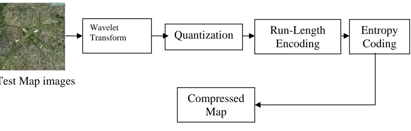
Figure 1.0: Steps of the Wavelet Image Compression Algorithm
A procedure for the corresponding four decompression steps will also be necessary in order to validate the benchmark. These corresponding steps (inverse wavelet
transform, dequantization, run-length decoding, and entropy decoding) must be performed in reverse order and will generate a new image file. Computing the peak signal-to-noise ratio of the new image based on the original will assess the quality of the compression algorithm. Since this decompression routine will only be used for validation purposes, it may be performed entirely in software.
The following restrictions apply to the implementation of each of the compression steps:
1. Wavelet Transform. Any wavelet transform and filter banks may be used for this step as long as the final algorithm meets the minimum compression and image quality
requirements specified by the acceptance tests (see section 5). Note that transforms other than wavelets (e.g., Fast Fourier Transform, Discrete Cosine Transform) may not be used.
2. Quantization. This step allows wavelet coefficients of small magnitude to be set to zero and reduces the number of distinct wavelet coefficients by mapping them to a smaller number of quantization indices. Since this step is inherently lossy, care must be taken to guarantee that enough information is retained to reconstruct the image at a high
Wavelet
Transform Quantization Run-Length Encoding
Entropy Coding
enough quality level. Acceptable quantization algorithms may be vector or scalar, uniform or adaptive.
3. Run-Length Encoding (RLE). Runs of repeated coefficients are compressed through runlength encoding. Either arbitrary RLE or zero RLE is acceptable for this step.
4. Entropy Coding. A final lossy compression step must be performed to reduce the size of the run-length encoded data. Acceptable entropy coding algorithms include Huffman, Shannon-Fano, and arithmetic coding. A host processor will copy each of the test image files to memory that is accessible to the configurable computing system under test (SUT). The host computer will then initiate a timer and send a signal to the SUT. This timer will be stopped as soon as the SUT signals termination. At that time, the host will copy image information back to disk, perform any remaining compression steps in software, generate a compressed image file, and carry out the acceptance tests. If the compressed image file is deemed acceptable, the elapsed compression time will be reported. As noted above, a corresponding software-based decompression procedure will be required for carrying out the acceptance test.
1.3OBJECTIVE
i. To study the image compression technique to be applied in Map Online system using Internet-based Image Catalogue
ii. To develop database for topographic
1.4SCOPE OF STUDY
CHAPTER II
LITERATURE STUDY
2.1 AN INTRODUCTION FOR WAVELETS
Digital maps carry along its geo-data such as coordinates, contour system, surface structures, and so on. High quality maps can retrieve essential information meaningful in Geographical Information System. It’s so easy to capture the high quality map images, but the complicated is when to store it. Because the high quality map image must be allocated and handled in a giant storage. The bigger size means the bigger capacity needed. This is not an economic way in storage systems. To preserve the quality and to reduce the storage usage, the map images should be compress first using a mathematical tool called Wavelet. Wavelets are mathematical functions that split up data into different frequency components, and then study each component with a resolution matched to its scale. Wavelets have more advantages than traditional Fourier Transforms methods in analyzing physical situations where the signal contains discontinuities and sharp spikes. Wavelets were developed independently in the fields of mathematics, images processing, quantum physics, electrical engineering, and seismic geology. There are a lot of new applications born because of the interchange. For instances the applications in image and data compression, turbulence, human vision, radar, and earthquake prediction. This chapter will describes the history of wavelets beginning with Fourier, compare wavelet transforms with Fourier Transforms, state properties and other special aspects of
of the contents focus on the application for image compression that applied to a very big size of map image data.
2.2 WAVELETS OVERVIEW
The fundamental idea behind wavelets is to analyze according to scale. The scale or sizes of the data cause the memory usage increase. Wavelets are functions that satisfy certain mathematical requirements and are used in representing data or other functions. This is not a new idea. Early 1800's, Joseph Fourier discovered that he could superpose sines and cosines to represent other functions. However, in wavelet analysis, the scale that used to look at data plays a special role. Wavelet algorithms process data at different scales or resolutions. The result in wavelet analysis is to see both the forest and the trees, so to speak. This makes wavelets interesting and useful.
fields that are making use of wavelets include astronomy, acoustics, nuclear engineering, sub-band coding, signal and image processing, neurophysiology, music, magnetic
resonance imaging, speech discrimination, optics, fractals, turbulence, earthquake-prediction, radar, human vision, and pure mathematics applications such as solving partial differential equations.
2.3 HISTORICAL PERSPECTIVE
In the history of mathematics, wavelet analysis shows many different origins. Much of the work was performed in the 1930s, and at the time, the separate efforts did not appear to be parts of a coherent theory.
2.3.1 PRE-1930
Before 1930, the main branch of mathematics leading to wavelets began with Joseph Fourier (1807) with his theories of frequency analysis, now often referred to as Fourier synthesis. He asserted that any 2π-periodic function f(x) is the sum
(1)
Fourier's assertion played an essential role in the evolution of the ideas mathematicians had about the functions.
After 1807, by exploring the meaning of functions, Fourier series convergence, and orthogonal systems, mathematicians gradually were led from their previous notion of frequency analysis to the notion of scale analysis. That is, analyzing f(x) by creating mathematical structures that vary in scale. How? Construct a function, shift it by some amount, and change its scale. Apply that structure in approximating a signal. Now repeat the procedure. Take that basic structure, shift it, and scale it again. Apply it to the same signal to get a new approximation. And so on. It turns out that this sort of scale analysis is less sensitive to noise because it measures the average fluctuations of the signal at
different scales.
The first mention of wavelets appeared in an appendix to the thesis of A. Haar (1909). One property of the Haar wavelet is that it has compact support, which means that it vanishes outside of a finite interval. Unfortunately, Haar wavelets are not continuously differentiable which somewhat limits their applications.
2.3.2 THE 1930S
Another 1930s research effort by Littlewood, Paley, and Stein involved computing the energy of a function f(x)
(2)
The computation produced different results if the energy was concentrated around a few points or distributed over a larger interval. This result disturbed the scientists because it indicated that energy might not be conserved. The researchers discovered a function that can vary in scale and can conserve energy when computing the functional energy. Their work provided David Marr with an effective algorithm for numerical image processing using wavelets in the early 1980s.
2.3.3 1960-1980
Between 1960 and 1980, the mathematicians Guido Weiss and Ronald R.
2.3.4 POST-1980
In 1985, Stephane Mallat gave wavelets an additional jump-start through his work in digital signal processing. He discovered some relationships between quadrature mirror filters, pyramid algorithms, and orthonormal wavelet bases (more on these later). Inspired in part by these results, Y. Meyer constructed the first non-trivial wavelets. Unlike the Haar wavelets, the Meyer wavelets are continuously differentiable; however they do not have compact support. A couple of years later, Ingrid Daubechies used Mallat's work to construct a set of wavelet orthonormal basis functions that are perhaps the most elegant, and have become the cornerstone of wavelet applications today.
2.4 FOURIER ANALYSIS
Fourier's representation of functions as a superposition of sines and cosines has become ubiquitous for both the analytic and numerical solution of differential equations and for the analysis and treatment of communication signals. Fourier and wavelet analysis have some very strong links.
2.4.1 FOURIER TRANSFORMS
Fourier transforms does just what you'd expect; transform data from the frequency domain into the time domain.
2.4.2 DISCRETE FOURIER TRANSFORMS
The Discrete Fourier Transform (DFT) estimates the Fourier transforms of a function from a finite number of its sampled points. The sampled points are supposed to be typical of what the signal looks like at all other times. The DFT has symmetry properties almost exactly the same as the continuous Fourier transform. In addition, the formula for the inverse discrete Fourier transform is easily calculated using the one for the discrete Fourier transform because the two formulas are almost identical.
2.4.3 WINDOWED FOURIER TRANSFORMS
If f(t) is a non-periodic signal, the summation of the periodic functions, sine and cosine, does not accurately represent the signal. You could artificially extend the signal to make it periodic but it would require additional continuity at the endpoints. The
Windowed Fourier transform (WFT) is one solution to the problem of better representing the non-periodic signal. The WFT can be used to give information about signals
simultaneously in the time domain and in the frequency domain.
interval's endpoints than in the middle. The effect of the window is to localize the signal in time.
2.4.4 FAST FOURIER TRANSFORMS
To approximate a function by samples, and to approximate the Fourier integral by the discrete Fourier transform, requires applying a matrix whose order is the number sample points n. Since multiplying an n x n matrix by a vector costs on the order of n2 arithmetic operations, the problem gets quickly worse as the number of sample points increases. However, if the samples are uniformly spaced, then the Fourier matrix can be factored into a product of just a few sparse matrices, and the resulting factors can be applied to a vector in a total of order n log n arithmetic operations. This is the so called Fast Fourier Transform or FFT (4).
2.5 WAVELET TRANSFORMS VERSUS FOURIER TRANSFORMS
2.5.1 SIMILARITIES BETWEEN FOURIER AND WAVELET TRANSFORMS
The Fast Fourier Transform (FFT) and the discrete wavelet transform (DWT) are both linear operations that generate a data structure that contains log2n segments of various lengths, usually filling and transforming it into a different data vector of length 2n.
and cosines. For the wavelet transform, this new domain contains more complicated basis functions called wavelets, mother wavelets, or analyzing wavelets. Both transforms have another similarity. The basis functions are localized in frequency, making mathematical tools such as power spectra (how much power is contained in a frequency interval) and scalegrams (to be defined later) useful at picking out frequencies and calculating power distributions.
2.5.2 DISSIMILARITIES BETWEEN FOURIER AND WAVELET TRANSFORMS
The most interesting dissimilarity between these two kinds of transforms is that individual wavelet functions are localized in space. Fourier sine and cosine functions are not. This localization feature, along with wavelets' localization of frequency, makes many functions and operators using wavelets “sparse" when transformed into the wavelet domain. This sparseness, in turn, results in a number of useful applications such as data compression, detecting features in images, and removing noise from time series.
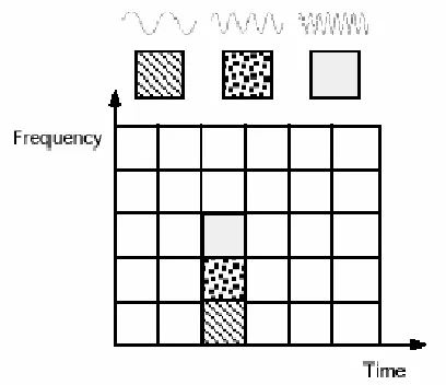
Fig. 2.1: Fourier basis functions, frequency tiles, and coverage of the time-frequency plane.
An advantage of wavelet transforms is that the windows vary. In order to isolate signal discontinuities, one would like to have some very short basis functions. At the same time, in order to obtain detailed frequency analysis, one would like to have some very long basis functions. A way to achieve this is to have short high-frequency basis functions and long low-frequency ones. This happy medium is exactly what you get with wavelet transforms. Figure 2.2 shows the coverage in the time-frequency plane with one wavelet function, the Daubechies wavelet.
Fig. 2.2: Daubechies wavelet basis functions, time-frequency tiles, and coverage of the time-frequency plane.
2.6 THE WAVELET SIGNAL FORM
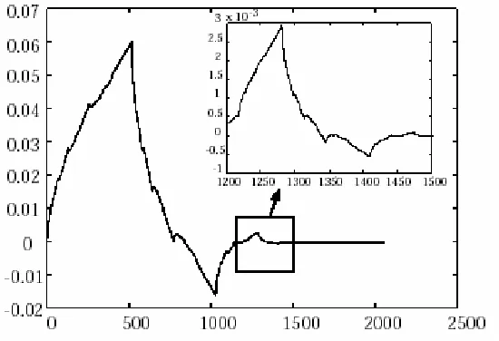
Wavelet transforms comprise an infinite set. The different wavelet families make different trade-offs between how compactly the basis functions are localized in space and how smooth they are. Some of the wavelet bases have fractal structure. The Daubechies wavelet family is one example (see Figure 2.3).
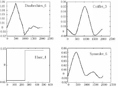
Within each family of wavelets (such as the Daubechies family) are wavelet subclasses distinguished by the number of coefficients and by the level of iteration. Wavelets are classified within a family most often by the number of vanishing moments. This is an extra set of mathematical relationships for the coefficients that must be satisfied, and is directly related to the number of coefficients (1). For example, within the Coiflet wavelet family are Coiflets with two vanishing moments, and Coiflets with three vanishing moments. In Figure 2.4, illustrates several different wavelet families.
2.7 WAVELET ANALYSIS
Now we begin our tour of wavelet theory, when we analyze our signal in time for its frequency content. Unlike Fourier analysis, in which we analyze signals using sines and cosines, now we use wavelet functions.
2.7.1 THE DISCRETE WAVELET TRANSFORM
Dilations and translations of the “Mother function," or “analyzing wavelet" Ф(x); define an orthogonal basis, our wavelet basis:
(3)
The variables s and l are integers that scale and dilate the mother function Ф to generate wavelets, such as a Daubechies wavelet family. The scale index s indicates the wavelet's width, and the location index l gives its position. Notice that the mother functions are rescaled, or “dilated" by powers of two, and translated by integers. What makes wavelet bases especially interesting is the self-similarity caused by the scales and dilations. Once we know about the mother functions, we know everything about the basis.
To span our data domain at different resolutions, the analyzing wavelet is used in a scaling equation:
(4)
(5)
where δ is the delta function and l is the location index.
One of the most useful features of wavelets is the ease with which a scientist can choose the defining coefficients for a given wavelet system to be adapted for a given problem. In Daubechies’ original paper (6), she developed specific families of wavelet systems that were very good for representing polynomial behavior. The Haar wavelet is even simpler, and it is often used for educational purposes.
It is helpful to think of the coefficients {c0
,…,
cn} as a filter. The filter or coefficients are placed in a transformation matrix, which is applied to a raw data vector. The coefficients are ordered using two dominant patterns, one that works as a smoothing filter (like a moving average), and one pattern that works to bring out the data's “detail" information. These two orderings of the coefficients are called a quadrature mirror filter pair in signal processing parlance. A more detailed description of the transformation matrix can be found elsewhere (4).2.7.2 THE FAST WAVELET TRANSFORM
The DWT matrix is not sparse in general, so we face the same complexity issues that we had previously faced for the discrete Fourier transform. We solve it as we did for the FFT, by factoring the DWT into a product of a few sparse matrices using
self-similarity properties. The result is an algorithm that requires only order n operations to transform an n-sample vector. This is the “fast" DWT of Mallat and Daubechies.
2.7.3 WAVELET PACKETS
The wavelet transform is actually a subset of a far more versatile transform, the wavelet packet transform. Wavelet packets are particular linear combinations of wavelets. They form bases, which retain many of the orthogonality, smoothness, and localization properties of their parent wavelets. The coefficients in the linear combinations are computed by a recursive algorithm making each newly computed wavelet packet coefficient sequence the root of its own analysis tree.
2.7.4 ADAPTED WAVEFORMS
According to Wickerhauser, some desirable properties for adapted wavelet bases are
1. Speedy computation of inner products with the other basis functions; 2. Speedy superposition of the basis functions;
3. Good spatial localization, so researchers can identify the position of a signal that is contributing a large component;
4. Good frequency localization, so researchers can identify signal oscillations; and 5. Independence, so that not too many basis elements match the same portion of the
signal.
For adapted waveform analysis, researchers seek a basis in which the coefficients, when rearranged in decreasing order, decrease as rapidly as possible. to measure rates of decrease, they use tools from classical harmonic analysis including calculation of information cost functions. This is defined as the expense of storing the chosen representation. Examples of such functions include the number above a threshold, concentration, entropy, and logarithm of energy, Gauss-Markov calculations, and the theoretical dimension of a sequence.
2.8 WAVELET APPLICATIONS
The following applications show just a small sample of what researchers can do with wavelets.
2.8.1 MAPONLINE SYSTEM PROTOTYPE
spread comprehensively also involved images or graphics with their attributes. Typically, the main problem in handling the geodatas of digital map is how to manage the size but still get the best quality. The best quality becomes the main point in GIS. Higher quality of the images means the data more accurate. So how to preserve this map image and to load in the Internet server? Geodatas is a retrieved data from map images and the images size are very big, especially the data in raster form because the data scanned at the high resolution (>600 dpi). For map online system, map image data in database normally topography and orthophoto images that could be view as an actual earth surface. For example, size of entire California using one-meter resolution and colored images were about 1.5TB or 1500GB.
Image data required high capacity of memory and space usage in server. So it’s become most problem in GIS. Basically, the data delivered in *.gif and *. jpeg format. To preserved and make the size smaller than actual size, the compression is needed. The compression method should destroy the image quality. One of the most popular
compression techniques is wavelet image compression. This technology affords to reduce the image size and preserved the image quality. Wavelet divides images to several
smaller blocks of data in decreasing the size. This technique also applied in software development. Using the technique, the image data delivered in *.wlt extension means the data already converted to wavelet form. In Map Online System, the *.wlt image data could be viewed using Java applets. A lot of data embedded with the data such as map series number, sheet number, scale, map edition and also the year of the images taken.
2.8.2 COMPUTER AND HUMAN VISION
scientific foundations for vision, and that while doing so, one must limit the scope of investigation by excluding everything that depends on training, culture, and so on, and focus on the mechanical or involuntary aspects of vision.
This low-level vision is the part that enables us to recreate the three-dimensional organization of the physical world around us from the excitations that stimulate the retina. Marr asked the questions:
• How is it possible to define the contours of objects from the variations of their light intensity?
• How is it possible to sense depth?
• How is movement sensed?
He then developed working algorithmic solutions to answer each of these questions. Marr's theory was that image processing in the human visual system has a complicated hierarchical structure that involves several layers of processing. At each processing level, the retinal system provides a visual representation that scales progressively in a
geometrical manner. His arguments hinged on the detection of intensity changes. He theorized that intensity changes occur at different scales in an image, so that their optimal detection requires the use of operators of different sizes.
2.8.2 FBI FINGERPRINT COMPRESSION
Between 1924 and today, the US Federal Bureau of Investigation has collected about 30 million sets of fingerprints. The archive consists mainly of inked impressions on paper cards. Facsimile scans of the impressions are distributed among law enforcement agencies, but the digitization quality is often low. Because a number of jurisdictions are experimenting with digital storage of the prints, incompatibilities between data formats have recently become a problem. This problem led to a demand in the criminal justice community for a digitization and compression standard.
In 1993, the FBI's Criminal Justice Information Services Division developed standards for fingerprint digitization and compression in cooperation with the National Institute of Standards and Technology, Los Alamos National Laboratory, commercial vendors, and criminal justice communities.
CHAPTER III
ALGORITHMS OF WAVELETS IN MAPONLINE
3.8 AN INTRODUCTION TO IMAGE COMPRESSIONS ALGORITHM
Compression is used just about everywhere. All the images we get in the web are compressed, typically in JPEG or GIF. In this chapter we will use the generic term messagefor the images we want to compress, which is the map images. The task of compression consists of two components, an encodingalgorithm that takes a message and generates a “compressed” representation (hopefully with fewer bits), and a decoding algorithm that reconstructs the original message or some approximation of it from the compressed representation. These two components are typically intricately tied together since they both have to understand the shared compressed representation. Everyone who’s involved in image processing knows that compression techniques produce either lossless or lossy results. We distinguish between lossless algorithms, which can
reconstruct the original message exactly from the compressed message, and lossy algorithms, which can only reconstruct an approximation of the original message.
they are imagining missing or switched pixel. Consider instead a system that reworded still images into a more standard form, or replaced that loss bit with synonyms so that the file can be better compressed. Technically the compression would be lossy since the image has changed, but the “meaning” and clarity of the message might be fully
maintained, or even improved. The explanations for this two types of compression can be referred in section 3.4 below.
There were a lot of image compression techniques in image processing. More techniques exists mean more algorithms was used. This chapter will describe about famous image compression algorithms, but only wavelet image compression will be explained
thoroughly. Comparison table attached to proof that the wavelet techniques more reliable. However because one can’t hope to compress everything, all compression algorithms must assume that there is some bias on the input messages so that some inputs are more likely than others, i.e.that there is some unbalanced probability distribution over the possible messages. Most compression algorithms base this “bias” on the structure of the messages i.e., an assumption that repeated characters are more likely than random characters, or that large white patches occur in “typical” images. Compression is therefore all about probability.
3.8 THE IMPORTANT OF COMPRESSIONS
The figures in Table 3.1 show the qualitative transition from simple text to full-motion video data and the disk space needed to store such uncompressed data
Table 3.1: Multimedia data types and uncompressed storage space required Multimedia Data Size/Duration Bits/Pixel or
Bits/Sample
Uncompressed Size A page of text 11'' x 8.5'' Varying resolution 16-32 Kbits Telephone quality
speech 1 sec 8 bps 64 Kbits
Color Image 512 x 512 24 bpp 6.29 Mbits Medical Image 2048 x 1680 12 bpp 41.3 Mbits SHD Image 2048 x 2048 24 bpp 100 Mbits Full-motion Video 640 x 480, 10
sec 24 bpp 2.21 Gbits
The examples above clearly illustrate the need for large storage space for digital image, audio, and video data. So, at the present state of technology, the only solution is to compress these multimedia data before its storage and transmission, and decompress it at the receiver for play back. With a compression ratio of 16:1, the space requirement can be reduced by a factor of 16 with acceptable quality.
3.8 PRINCIPLES OF COMPRESSION
A common characteristic of most images is that the neighboring pixels are highly correlated and therefore contain highly redundant information. The foremost task then is to find an image representation in which the image pixels are decorrelated. Redundancy and irrelevancy reductions are two fundamental principles used in compression. Whereas redundancy reduction aims at removing redundancy from the signal source
(image/video), irrelevancy reduction omits parts of the signal that will not be noticed by the signal receiver (viz. HVS). In general, three types of redundancy in digital images and video can be identified:
• Spatial Redundancy or correlation between neighboring pixel values.
• Spectral Redundancy or correlation between different color planes or spectral bands.
Image compression research aims at reducing the number of bits needed to represent an image by removing the spatial and spectral redundancies as much as
possible. Since in this article, we will focus only on still image compression, we will not worry about temporal redundancy.
3.8 TYPES OF COMPRESSION
(a) Lossless vs. Lossy compression: There are different ways of classifying compression techniques. Two of these would be mentioned here. The first categorization is based on the information content of the reconstructed image. They are 'lossless compression' and 'lossy compression' schemes. In lossless compression, the reconstructed image after compression is numerically identical to the original image on a pixel-by-pixel basis. However, only a modest amount of compression is achievable in this technique. In lossy compression on the otherhand, the reconstructed image contains degradation relative to the original, because redundant information is discarded during compression. As a result, much higher compression is achievable, and under normal viewing conditions, no visible loss is perceived (visually lossless).
compression compared to predictive methods, although at the expense of greater computations.
3.8 LOSSY COMPRESSION TECHNIQUES
Lossy compression is compression in which some of the information from the original message sequence is lost. This means the original sequences cannot be
regenerated from the compressed sequence. Just because information is lost doesn’t mean the quality of the output is reduced. For example, random noise has very high information content, but when present in an image or a sound file, we would typically be perfectly happy to drop it. Also certain losses in images or sound might be completely
imperceptible to a human viewer (e.g. the loss of very high frequencies). For this reason, lossy compression algorithms on images can often get a factor of 2 better compression than lossless algorithms with an imperceptible loss in quality. However, when quality does start degrading in a noticeable way, it is important to make sure it degrades in a way that is least objectionable to the viewer (e.g., dropping random pixels is probably more objectionable than dropping some color information). For these reasons, the way most lossy compression techniques are used are highly dependent on the media that is being compressed. Lossy compression for sound, for example, is very different than lossy compression for images.
In this section we go over some general techniques that can be applied in various contexts, and in the next two sections we go over more specific examples and techniques.
Figure 3.1: A Typical Lossy Signal/Image Encoder
Over the years, a variety of linear transforms have been developed which include Discrete Fourier Transform (DFT), Discrete Cosine Transform (DCT)[1], Discrete Wavelet Transform (DWT)[36] and many more, each with its own advantages and disadvantages. A thorough and excellent analysis of DCT and other related transforms and their applications can be found in [26]. A quantizer simply reduces the number of bits needed to store the transformed coefficients by reducing the precision of those values. Since this is a many-to-one mapping, it's a lossy process and is the main source of compression in an encoder. Quantization can be performed on each individual coefficient, which is known as Scalar Quantization (SQ). Quantization can also be performed on a group of coefficients together, and this is known as Vector Quantization (VQ). Both, uniform and non-uniform quantizers can be used depending on the problem at hand. For a thorough analysis on different quantization schemes, see section 3.51. An entropy encoder further compresses the quantized values losslessly to give better overall compression. Most commonly used entropy encoders are the Huffman encoder and the Arithmetic encoder, although for applications requiring fast execution, simple run-length coding has proven very effective. A nice overview on various entropy
3.8.1 Scalar Quantization
A simple way to implement lossy compression is to take the set of possible messages S and reduce it to a smaller set S’ by mapping each element of S to an element in S’. For example we could take 8-bit integers and divide by 4 (i.e., drop the lower two bits), or take a character set in which upper and lowercase characters are distinguished and replace all the uppercase ones with lowercase ones. This general technique is called quantization. Since the mapping used in quantization is many-to-one, it is irreversible and therefore lossy. In the case that the set S comes from a total order and the total order is broken up into regions that map onto the elements of S’, the mapping is called scalar quantization. The example of dropping the lower two bits given in the previous paragraph is an example of scalar quantization.
Applications of scalar quantization include reducing the number of color bits or gray-scale levels in images (used to save memory on many computer monitors), and classifying the intensity of frequency components in images or sound into groups (used in JPEG compression). In fact we mentioned an example of quantization when talking about JPEG-LS. Their quantization is used to reduce the number of contexts instead of the number of message values. In particular we categorized each of 3 gradients into one of 9 levels so that the context table needs only M Ý entries (actually only (93 + 1) / 2 due to symmetry).
probability of different input values. In fact, this idea can be formalized—for a given error metric and a given probability distribution over the input values, we want a mapping that will minimize the expected error. For certain error-metrics, finding this mapping might be hard. For the root-mean-squared error metric there is an iterative algorithm known as the Lloyd-Max algorithm that will find the optimal mapping. An interesting point is that finding this optimal mapping will have the effect of decreasing the effectiveness of any probability coder that is used on the output. This is because the mapping will tend to more evenly spread the probabilities in S’.
3.8.2 Vector Quantization
Scalar quantization allows one to separately map each color of a color image into a smaller set of output values. In practice, however, it can be much more effective to map regions of 3-d color space into output values. By more effective we mean that a better compression ratio can be achieved based on an equivalent loss of quality.
The general idea of mapping a multidimensional space into a smaller set of
messages S’ is called vector quantization. Selecting a set of representatives from the input space, and then mapping all other points in the space to the closest representative
typically implement vector quantization. The representatives could be fixed for all-time and part of the compression protocol, or they could be determined for each file (message sequence) and sent as part of the sequence. The most interesting aspect of vector
quantization is how one selects the representatives. Typically it is implemented using a clustering algorithm that finds some number of clusters of points in the data. A
representative is then chosen for each cluster by either selecting one of the points in the cluster or using some form of centroid for the cluster. Finding good clusters is a whole interesting topic on its own.
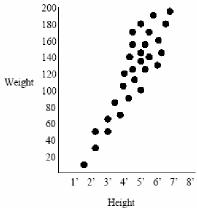
height-weight chart. There is clearly a strong correlation between people’s height and weight and therefore the representatives can be concentrated in areas of the space that make physical sense, with higher densities in more common regions. Using such
representatives is very much more effective than separately using scalar quantization on the height and weight.
Figure 3.2: Example of vector quantization for a height-weight chart.
We should note that vector quantization, as well as scalar quantization, can be used as part of lossless compression technique. In particular if in addition to sending the closest representative, the coder sends the distance from the point to the representative, then the original point can be reconstructed. The distance is often referred to as the residual. In general this would not lead to any compression, but if the points are tightly clustered around the representatives, then the technique can be very effective for lossless compression since the residuals will be small and probability coding will work well in reducing the number of bits.
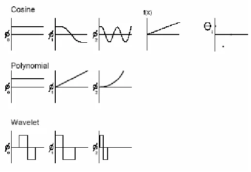
The idea of transform coding is to transform the input into a different form which can then either be compressed better, or for which we can more easily drop certain terms without as much qualitative loss in the output. One form of transform is to select a linear set of basis functions (Øi) that span the space to be transformed. Some common sets include sin, cos, polynomials, spherical harmonics, Bessel functions, and wavelets. Figure 3.2 shows some examples of the first three basis functions for discrete cosine, polynomial, and wavelet transformations. For a set of n values, transforms can be expressed as an n x n matrix T. Multiplying the input by this matrix T gives, the
transformed coefficients. Multiplying the coefficients by T-1 will convert the data back to the original form. For example, the coefficients for the discrete cosine transform (DCT) are
The DCT is one of the most commonly used transforms in practice for image
compression, more so than the discrete Fourier transform (DFT). This is because the DFT assumes periodicity, which is not necessarily true in images. In particular to represent a linear function over a region requires many large amplitude high-frequency components in a DFT. This is because the periodicity assumption will view the function as a
Figure 3.3: Transforms
For the purpose of compression, the properties we would like of a transform are 1. To decorrelate the data,
2. have many of the transformed coefficients be small, and
3. have it so that from the point of view of perception, some of the terms are more important than others.
3.6 WAVELET IMAGE COMPRESSION
JPEG decompose images into sets of cosine waveforms. Unfortunately, cosine is a periodic function; this can create problems when an image contains strong aperiodic features. Such local high-frequency spikes would require an infinite number of cosine waves to encode properly. JPEG and MPEG solve this problem by breaking up images into fixed-size blocks and transforming each block in isolation. This effectively clips the infinitely repeating cosine function, making it possible to encode local features.
applied to the entire image, without requiring blocking and without degenerating when presented with high-frequency local features.
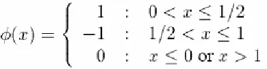
How do we derive a suitable set of basis functions? We start with a single function, called a “mother function”. Whereas cosine repeats indefinitely, we want the wavelet mother function,
ø,
to be contained within some local region, and approach zero as we stray further away:The families of basis functions are scaled and translated versions of this mother function. For some scaling factor s and translation factor l,
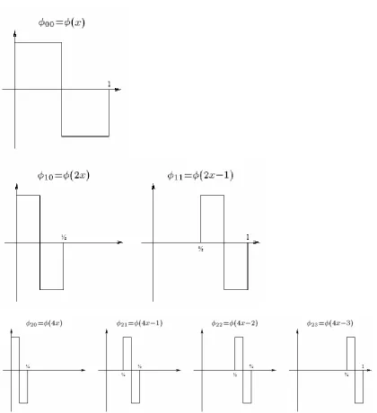
A well know family of wavelets are the Haar wavelets, which are derived from the following mother function:
Figure 3.4: A small Haar wavelet family of size seven.
Figure 3.5: A sampling of popular wavelet
3.6.1 WAVELET IN THE REAL WORLD
Summus Ltd. is the premier vendor of wavelet compression technology. Summus claims to achieve better quality than JPEG for the same compression ratios, but has been loathe divulging details of how their wavelet compression actually works. Summus wavelet technology has been incorporated into such items as:
• Wavelets-on-a-chip for missile guidance and communications systems.
• Image viewing plugins for Netscape Navigator and Microsoft Internet Explorer.
• Desktop image and movie compression in Corel Draw and Corel Video.
• Digital cameras under development by Fuji.
In a sense, wavelet compression works by characterizing a signal in terms of some underlying generator. Thus, wavelet transformation is also of interest outside of the realm of compression. Wavelet transformation can be used to clean up noisy data or to detect self-similarity over widely varying time scales. It has found uses in medical imaging, computer vision, and analysis of cosmic X-ray sources.
3.7 IMPLEMENTING WAVELET IN MAPONLINE
Wavelet techniques were chosen among the other compression techniques. The result of the comparison between Wavelet, Jpeg, and Tiff technique has been studied. Wavelet result is better than others in compressing the map images.
3.7.1 WAVELET COMPRESSION ALGORITHM FOR MAPONLINE
text, experiment results, or object compiled code. The lossy compression algorithm will discard unused data to reduce the data or image size. Normally implemented for images and digital sound file.
To compress map image in Map Online System, lossy compression algorithm was used because the discarded data could not be vision by naked eye. Almost of this
3.8 OTHER TYPES OF LOSSY IMAGE COMPRESSION TECHNIQUES
3.8.1 JPEG (Joint Photographic Experts Group)
JPEG is a lossy compression scheme for color and gray-scale images. It works on full 24-bit color, and designed to be used with photographic material and naturalistic artwork. It is not the ideal format for line drawings, textual images, or other images with large areas of solid color or a very limited number of distinct colors. The lossless
techniques, such as JBIG, work better for such images. JPEG is designed so that the loss factor can be tuned by the user to tradeoff image size and image quality, and is designed so that the loss has the least effect on human perception. It however does have some anomalies when the compression ratio gets high, such as odd effects across the
boundaries of 8x8 blocks. For high compression ratios, other techniques such as wavelet compression appear to give more satisfactory results.
Figure 3.3: Steps in JPEG compression
The next step of the JPEG algorithm is to partition each of the color planes into 8x8 blocks. Each of these blocks is then coded separately. The first step in coding a block is to apply a cosine transform across both dimensions. This returns an 8x8 block of 8-bit frequency terms. So far this does not introduce any loss, or compression. The block-size is motivated by wanting it to be large enough to capture some frequency components but not so large that it causes “frequency spilling”. In particular if we cosine-transformed the whole image, a sharp boundary anywhere in a line would cause high values across all frequency components in that line. After the cosine transform, the next step applied to the blocks is to use uniform scalar quantization on each of the frequency terms. This
quantization is controllable based on user parameters and is the main source of
information loss in JPEG compression. Since the human eye is more perceptive to certain frequency components than to others, JPEG allows the quantization scaling factor to be different for each frequency component. The scaling factors are specified using an 8x8 table that simply is used to element-wise divide the 8x8 table of frequency components. JPEG defines standard quantization tables for both the Y and I-Q components.
The table for Y is shown in Table 3.1. In this table the largest components are in the lower-right corner. This is because these are the highest frequency components which humans are less sensitive to than the lower-frequency components in the upper-left corner. The selection of the particular numbers in the table seems magic, for example the table is not even symmetric, but it is based on studies of human perception.
If desired, the coder can use a different quantization table and send the table in the head of the message. To further compress the image, the whole resulting table can be divided by a constant, which is a scalar “quality control” given to the user. The result of the quantization will often drop most of the terms in the lower left to zero. JPEG
better compression. The other components (the AC components) are now compressed. They are first converted into a linear order by traversing the frequency table in a zig-zag order (see Figure 3.4). The motivation for this order is that it keeps frequencies of approximately equal length close to each other in the linear-order. In particular most of the zeros will appear as one large contiguous block at the end of the order. A form of run-length coding is used to compress the linear-order. It is coded as a sequence of
(skip,value) pairs, where skip is the number of zeros before a value, and value is the value. The special pair (0,0) specifies the end of block. For example, the sequence
[4,3,0,0,1,0,0,0,1,0,0,0,...] is represented as [(0,4),(0,3),(2,1),(3,1),(0,0)]. This sequence is then compressed using either arithmetic or Huffman coding. Which of the two coding schemes used is specified on a per-image basis in the header.
16 11 10 16 24 40 51 61 12 12 14 19 26 58 60 55 14 13 16 24 40 57 69 56 14 17 22 29 51 87 80 62 18 22 37 56 68 109 103 77 24 35 55 64 81 104 113 92 49 64 78 87 103 121 120 101 72 92 95 98 112 100 103 99
Figure 3.4: Zig-zag scanning of JPEG blocks
3.8.2 FRACTAL COMPRESSION
A function f(x) is said to have a fixed xfif xf=f(xf). For example:
This was a simple case. Many functions may be too complex to solve directly. Or a function may be a black box, whose formal definition is not known. In that case, we might try an iterative approach. Keep feeding numbers back through the function in hopes that we will converge on a solution:
For example, suppose that we have f(x) as a black box. We might guess zero as x0 and iterate from there:
x0 0
x1 f(x0) = 1
x2 f(x1) = 1.5
x3 f(x2) = 1.75
x5 f(x4) = 1.9375
x6 f(x5) = 1.96875
x7 f(x6) = 1.984375
x8 f(x7) = 1.9921875
In this example, f(x) was actually defined ½ x + 1. The exact fixed point is 2, and the iterative solution was converging upon this value. Iteration is by no means guaranteed to find a fixed point. Not all functions have a single fixed point. Functions may have no fixed point, many fixed points, or an infinite number of fixed points. Even if a function has a fixed point, iteration may not necessarily converge upon it. In the above example, we were able to associate a fixed-point value with a function. If we were given only the function, we would be able to recompute the fixed-point value. Put differently, if we wish to transmit a value, we could instead transmit a function that iteratively converges on that value.
This is the idea behind fractal compression. However, we are not interested in transmitting simple numbers, like “2”. Rather, we wish to transmit entire images. Our fixed points will be images. The functions, then, will be mappings from images to images. The encoder will operate roughly as follows:
1. Given an image, i, from the set of all possible images, Image. 2. Compute a function f : Image Æ Image such as f(i) ≈ i. 3. Transmit the coefficients that uniquely identify f.
Now, the decoder will use the coefficients to reassemble f and reconstruct its fixed point, the image:
1. Receive coefficients that uniquely identify some function f: Image Æ Image. 2. Iterate f repeatedly until its value converges on a fixed image, i.
Figure 3.5: Identifying self-similarity. Range blocks appear on the left; one domain block appears on the left. The arrow identifies one of several collage function that
would be composites into a complete image.
Clearly we will not be using entirely arbitrary functions here. We want to choose functions from some family that the encoder and decoder have agreed upon in advance. The members of this family should be identifiable simply by specifying the values for a small number of coefficients. The functions should have fixed points that may be found via iteration, and must not take unduly long to converge.
Figure 3.5 shows a simplified example of decomposing an image info collage of itself. Note that the encoder starts with the subdivided image on the right. For each “range” block, the encoder searchers for a similar “domain” block elsewhere in the image. We generally want domain blocks to be larger than range blocks to ensure good convergence at decoding time.
3.8.3 MODEL-BASED COMPRESSION
CHAPTER IV
IMPLEMENTATION OF WAVELET IMAGE COMPRESSION IN MAP ONLINE PROTOTYPE
4.1 INTRODUCTION
As mentioned before, Map Online System Prototype was the prototype system for end-user to get information their place around. All maps image will be displayed in catalogue system. Registered users can access the map all over Malaysia by upgrading their level in this system. For the first 15 days, users will give free evaluation registration. But user is unable to make purchasing for the map. The limited registration permits users only for viewing the all Malaysia maps only for 15 days. This chapter will describe about process in development of Map Online System Prototype thoroughly.
4.2 PLANNING FOR MAPONLINE
4.2.1 DATABASE PLANNING
instances SQL Server, PostgreSQL, MySQL, and so on. But for Map Online System Prototype, MySQL database had chosen to manage data and designing database structure. Compatibility of MySQL and PHP Hypertext Preprocessor (PHP) make it more
convenient to manage. For the system, the vision of database planning is to design database using MySQL that could be used to store topographic maps and thematic. From the observations on the other system, it also applied the common concept. Database planning was useful to detect every weakness and strength of the system as a guideline for the thorough development phase. Figure 4.1 shows the process in database planning.
Figure 4.1: Database Planning Activities
4.3 SYSTEM VISUALIZATION
Organization situation analysis
Organization operation
Organization operation
Organization operation
Defining problems and constraints
4.3.1 CONTEXT DIAGRAM
MapOnline System is a critical system that needs a solid visual view. This view has to be switched to actual system. Context diagram created to visualize the relationship between outside entity and Maponline System. Outside entity consists of personnel or other system that interacts with MapOnline. Context diagram was Top-Level View in Information System. All outside entity located around the process parameter and
connected by data flow. Storage data could not viewed because it was internal process in MapOnline. Figure 4.1 shows to entity, System User and System Administrator
connected to MapOnline system by data flow.
System User
System Administrator 0
MapOnline System Prototype
D 1.5
Registration
D 1.1
Login
D 1.2 Application
List
D 1.3 User Information
D 1.4
Approval
P1 New application
Submit registration
Update database Verify login
Retrieve data Retrieve data System
Admin System User
Login to system
Check new application
Display user information
Approve new user
System Administrator
D1
Application
D2
Renewing Application
D3
Reports
D4
Maintenance
D5
Online Status
P1 User System
System Administrator System User D1 Registration D2 Update D3 Map D4 Metadata Search D5 Catalogue D6 Feedback D7 Plugin P1 User System P2 Topogra phy P3 database Java Applett
Feedback to webmaster View map by sheet no.
View map by metadata search
Submit to system user First time registration
Update particular record
View map by series no.
Data stored and checked by system admin
Display user information Update database
Get from database
Get from database
Get from database
Get from database
Maintain database
4.3 USER INTERFACE FOR MAP ONLINE SYSTEM PROTOTYPE
4.3.1 Main Page
4.3.2 Maps Registration Page
CHAPTER V
CONCLUSION
A. Project Identification 1. Project number : 75080
2. Project title : Map Online System Using Internet-based Image Catalogue 3. Project Leader : Encik Noor Azam bin Md Sheriff
B. Type of research
Indicate the type of research of the project (Please see definitions in the Guidelines for completing the Application Form)
√ Scientific research (fundamental research)
Technology development (applied research)
Product/process development (design and engineering) Social/policy research
C. Objectives of the project 1. Socio-economic objectives
Which socio-economic objectives are addressed by the project? (Please identify the sector, SEO Category and SEO Group under which the project falls. Refer the
Malaysian R&D Classification System brochure for SEO Group code)
Sector : 9 SEO Category : 1
SEO Group and Code : S 50105 2. Fields of research
Which are the two main FOR Categories, FOR Group, and FOR Areas of your project? (Please refer to the Malaysia R&D Classification System brochure for the FOR Group Code)
a. Primary field of research FOR Category: F10500
FOR Group and Code: Information Systems F10501
FOR Group and Code: Current Information Technology F10504 FOR Area: Others current information technology
D. Project duration
What was the duration of the project?
1 February 2004 – 31 January 2005 (12 months)
E. Project manpower
How many man-months did the project involve?
F. Project costs
What were the total project expenses of the project RM 24,000.00
G. Project funding
Which were the funding sources for the project?
A. Technical contribution of the project
1. What was the achieved direct output of the project: For scientific (fundamental) research projects?
Algorithm Structure Data
Other, Please specify:
_______________________________________________
For technology development (applied research) project: Method/technique
Demonstrator/prototype Other, Please specify:
_______________________________________________
For product/process development (design and engineering) projects: Product/component
Process Software
Other, Please specify:
_______________________________________________
2. How would you characterize the quality of this output? Significant breakthrough
Major improvement Minor improvement
√
√
√
1. How has the output of the project been documented? Detailed project report
Product/process specification documents Other, please specify:
_______________________________________________
2. Did the project create an intellectual property stock? Patent obtained
Patent pending
Patent application will be filed Copyright
3. What publications are available?
Articles (s) in scientific publications How many: Papers (s) delivered at conferences/seminars How many: Book
√ Other, Please specify: Technical report for RMC
4. How significant are citations of the results?
Citations in national publications How many: Citations in international publications How many:
Not Yet
Not known
√
√
A. Contribution of the project to expertise development 1. How did the project contribute to expertise?
PhD degrees How many: MSc degrees How many: Research staff with new specialty How many: 1 Other, Please specify:
________________________________________________ 2. How significant is this expertise?
One of the key areas of priority for Malaysia An important area, but not a priority one
B. Economic contribution of the project?
1. How has the economic contribution of the project materialized? Sales of manufactured product/equipment
Royalties from licensing Cost saving
Time saving Other, Please specify:
_________________________________________________ 2. How important is this economic contribution?
High economic contribution Value : RM Medium economic contribution Value : RM 80,000 Low economic contribution Value : RM
3. How important is this economic contribution? Already materialized
1. What infrastructural contribution has the project had? New equipment Value : RM New/improved facility Investment : RM New information networks
Other, Please specify:
_________________________________________________ 2. How significant is this infrastructural contribution for the organization?
Not significant/does not leverage other projects Moderately significant
Very significant/significantly leverages other projects
D. Contribution of the project to the organization’s reputation
1. How has the project contributed to increasing the reputation of the organization
Recognition as a Centre of Excellence National award
International award Demand for advisory services
Invitations to give speeches on conferences Visits from other organization
Other, Please specify:
_________________________________________________ 2. How important is the project’s contribution to the organization’s
reputation?
Not significant
Moderately significant Very significant
√
√
√
A. Contribution of the project to organizational linkages 1. Which kinds of linkages did the project create?
Domestic industry linkages International industry linkages
Linkages with domestic research institutions, universities Linkages with international research institutions, universities
2. What is the nature of the linkages Staff exchanges
Inter-organizational project team Research contract with a commercial client Informal consultation
Other, Please specify:
B. Social-economic contribution of the project
1. Who are the direct customer/beneficiaries of the project output?
Customers/beneficiaries: Number:
√
Improvements in health Improvements in safety
Improvements in the environment
Improvements in the energy consumption Improvements in the international relations Other, Please specify:
Improve in provision of IT services
3. How important is this socio-economic contribution? High social contribution
Medium social contribution Low social contribution
4. When has/will this social contribution materialized? Already materialized
Within three years of project completion Expected in three years or more
Unknown
Date: Signature:
√ √
A. Purpose
The purpose of the End of Project is to allow the IRPA Panels and their supporting group of experts to assess the results of research projects and the technology transfer actions to be taken.
B. Information Required
The following Information is required in the End of Project Report :
• Project summary for the Annual MPKSN Report; • Extent of achievement of the original project objectives; • Technology transfer and commercialisation approach;
• Benefits of the project, particularly project outputs and organisational outcomes; and • Assessment of the project team, research approach, project schedule and project
costs.
C. Responsibility
The End of Project Report should be completed by the Project Leader of the IRPA-funded project.
D. Timing
The End of Project Report should be submitted within three months of the completion of the research project.
E. Submission Procedure
One copy of the End of Project is to be mailed to :
IRPA Secretariat
Ministry of Science, Technology and the Environment 14th Floor, Wisma Sime Darby
A. Project number:75080
Project title:Map Online System Using Internet-based Image Catalogue
Project leader:Encik Noor Azam bin Md Sheriff
Tel: 07 – 5532322 Fax: 07 – 5565044
B. Summary for the MPKSN Report (for publication in the Annual MPKSN Report, please summarise
the project objectives, significant results achieved, research approach and team strucure)
Digital maps carry along its geodata information such as coordinate that is important in one particular topographic and thematic map. These geodatas are meaningful especially in a military field. Usually, the size of this map is big and need a big storage to store this data in the database. Thus, its will take more time for data downloading process using an image catalogue approach on the internet. According to time consuming and data transmitting factor, we used an image compression techniques to solve the problem. On the other hand, a comparisons study of image compression techniques for geodata such as topographic and thematic map has been done. With image compression techniques, the storage size of the image can be reduced without affected the quality of the image. This research focused on image compression techniques using wavelet technology. As a result, the compressed images will be applied to a system called Map Online. A benchmarking of the result for the compressed geodata transmitting over intranet and Internet connection has been done to prove the reliability of the techniques. The knowledge gathered from this study is very useful to for JUPEM and others government agency to implement a Map Online System in order to produce higher quality of images data transmitting.