Development of a Precision Neutron Lifetime Measurement: Magnetic Trapping of Ultracold Neutrons.

(1)

P. R. Huﬀman).

(2)

by

Christopher Martin O’Shaughnessy

A dissertation submitted to the Graduate Faculty of North Carolina State University

in partial fullfillment of the requirements for the Degree of

Doctor of Philosophy

Physics

Raleigh, North Carolina

2010

APPROVED BY:

Dr. David G. Haase Dr. Gail C. McLaughlin

(3)

Biography

Christopher M. O’Shaughnessy was born in upstate NY to two cool and loving parents somewhere between 1978 and 1985. He has one older brother who knits amazingly well. Early in life, Chris gained notoriety for pink striped pajamas

(4)

Acknowledgements

I would like to thank Paul Huﬀman for the outstanding support he has oﬀered me when I needed it most and for the freedom he has given me in those times when his support was not necessary. My experience would not have been as valuable without the assortment of opportunities that Paul has made available to me.

Without the passion for physics from individuals such as Albert Young and Robby Pattie, I do not think my excitement for physics would have persisted as long as it has. The long hours and hard labor of a work often obscure the reasons for completing it. For reminding me so vividly of the global picture I am indebted to them.

Thank you also to my committee members, Professors Gould, Haase, and McLaugh-lin for sharing your time and experience with me.

I am grateful to Pieter Mumm for sharing with me both his technical experience and his friendship. Without the groundwork layed out by Liang Yang, I would have made very little progress. His hardly questionable advice, good safety record, and impressive crossword skills were a standard to live up to. For the the always witful life advice from Jeﬀrey Nico I am also indebted.

I must also acknowledge my NCSU oﬃcemates Adam Holley, Grant Palmquist, Robby Pattie, Peter Gilbert, Keith Heyward, and Liping Yu; without whose furniture rear-rangements I wouldn’t quite have the right perspective for a career in physics. I would also like to thank Karl Schelhammer, Michael Huber, Patrick Hughes, Nathan Meyer, Dmitryi Lyapustin, Craig Huﬀer, Courtney Taylor and Daniel Marley for all of their contributions to this work.

(5)

List of Figures

Figure 1.1 An example of a symmetry breaking potential, the ‘mexican hat’

potential . . . 12

Figure 1.2 Feynman diagram for neutronβ-decay. . . 18

Figure 1.3 The f tvalues of 20 superallowed nuclearβ-decays. . . 23

Figure 1.4 The time evolution of the NSE abundances of the nuclides of interest. 27 Figure 1.5 Light element abundances; BBN calculation, and observations. . . . 28

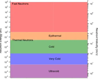
Figure 2.1 Classiﬁcation of neutron energies, and velocities. . . 31

Figure 2.2 A timeline of neutron lifetime measurements . . . 33

Figure 2.3 An exclusion plot of the couplings gaand gv. . . 35

Figure 2.4 Schematic of the NIST neutron lifetime beam measurement. . . 37

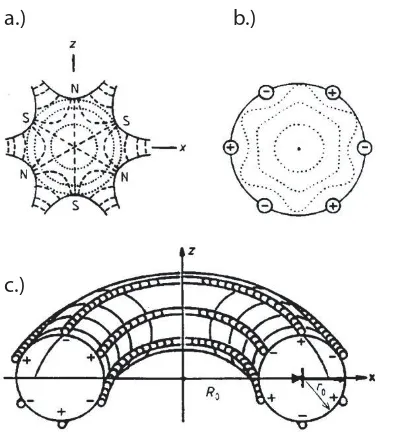
Figure 2.5 Schamatic of a sextupole ﬁeld and potential. . . 40

Figure 2.6 Permanent magnet gravitrap . . . 42

Figure 2.7 Neutron trapping data taken with the Mark II apparatus . . . 45

Figure 3.1 The dispersion curves for both the free neutron and superﬂuid helium. 48 Figure 3.2 Layout of the NG-6 neutron guide. . . 49

Figure 3.3 Spectrum of the neutrons reﬂected by the NG-6U monochromator . 50 Figure 3.4 A photograph of the assembled Ioﬀe trap. . . 53

Figure 3.5 Circuit diagram for the active quench protection of the quadrupole magnet. . . 55

Figure 3.6 Top view photograph of one ﬁeld compensating solenoid magnet. . . 57

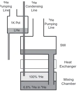
Figure 3.7 Schematic of the operation of a dilution refrigerator. . . 58

Figure 3.8 A cross sectional view of the cryostat. . . 61

Figure 3.9 Schematic of the Fermilab HTS current leads. . . 63

Figure 3.10 HTS high current leads quench detection . . . 65

Figure 3.11 A side view of the neutron entrance and shielding materials. . . 68

Figure 3.12 A cross section of the experimental cell. . . 72

Figure 3.13 A top view of the new light collection system. . . 74

Figure 3.14 Lambert’s cosine law. . . 75

(8)

paper walls. . . 79

Figure 3.17 A comparison of simulation and data . . . 81

Figure 3.18 Light Collection System from the previous apparatus. . . 82

Figure 3.19 Eﬃciency throughout the collection system as a function of source position. . . 83

Figure 3.20 The light collection eﬃciency in the Mark II apparatus after the 77 K guide. . . 85

Figure 3.21 Detection eﬃciency as a function of axial position within the cell of the new apparatus. . . 86

Figure 3.22 Neutron time-of-ﬂight measurements with the reﬂective polymer vikuiti in the beam. . . 89

Figure 3.23 Neutron transmission through the Vikuiti polymer showing the char-acteristic 1/vdependence. . . 89

Figure 3.24 Finite element analysis of the cell optical window. . . 91

Figure 3.25 Photograph of the 77 K light guide element. . . 92

Figure 3.26 A time line of the major events during the run schedule. . . 93

Figure 3.27 The digitized waveform of a typical PMT pulse. . . 95

Figure 3.28 The DAQ interface with the SCRs to energize the magnets. . . 98

Figure 3.29 The relative directional dependance of the origin of background events.104 Figure 3.30 The pulse height spectrum from PMTβ data in the MarkII apparatus.105 Figure 4.1 Magnetic ﬁeld simulations of the KEK trap. . . 113

Figure 4.2 Loss probability for a neutron incident on a semi-inﬁnite plane of Tetraphenyl Butadiene. . . 115

Figure 4.3 A complex material potential of many steps . . . 116

Figure 4.4 Loss probability for a neutron incident on the multi-layered cell wall. 118 Figure 4.5 The boundary of a rough surface may be treated as a perturbation to the ﬂat plane . . . 119

Figure 4.6 The loss probability for neutrons incident on a porous Gore-Tex material.122 Figure 4.7 The surface roughness of TPB evaporated on aG_or-T_{ex substrate. .} ₁₂₃

Figure 4.8 Ramping schedules used in studies of above threshold neutrons. . . . 126

(9)

List of Tables

Table 1.1 Weak hypercharge of the fermion ﬁelds. . . 16

Table 1.2 Fermi and Gamow-Teller decay mode transitions. . . 21

Table 3.1 Parameters of the new Ioﬀe-type magnet trap. . . 52

Table 3.2 Activation analysis of the Vikuiti ESR material. . . 88

Table 3.3 Status of the magnets at initiation of each of the quenches. . . 102

Table 4.1 Properties of the materials in the experimental cell. . . 123

Table 4.2 Surface character of the detector insert materials. . . 124

(10)

Chapter 1

Introduction

This thesis describes advancements made in a technique for measuring the neu-tron lifetime using magnetically trapped ultracold neuneu-trons. The neuneu-tron lifetime plays an important role in both nuclear astrophysics and in the standard model of particle physics. Chapter 1 describes the theory of β-decay in detail, and explains the motivations in both of these topics. A discussion of the common techniques used for measuring the neutron lifetime and an analysis of their results can be found in Chapter 2. To address the short-comings of these techniques a new method that employs magnetic trapping of UCN has been developed.

The knowledge gained from two apparatuses built and operated before this thesis work was used in the design of a new apparatus that is now ready to make a precision measurement of the neutron lifetime. While the previous traps have demonstrated the feasibility of the measurement technique, they were statistically limited from making a precise measurement of the neutron lifetime. The key improvement in the new apparatus is a larger and deeper magnetic trap that utilizes a high-current superconducting quadrupole magnet in an Ioﬀe conﬁguration. The resulting gain is in the number of neutrons trapped in each run. Details of the design, construction, and commissioning of a new cryostat to support this trap can be found in Chapter 3. Optimizations of the signal collection and background shielding of this apparatus are also discussed here.

(11)

of ultracold neutrons is one of the largest systematic uncertainties in the experiment. To reduce the uncertainty associated with this, a direct measurement of the isotopic purity of the helium using accelerator mass spectroscopy will be described. The second largest effect comes from neutrons that escape the trap. Also discussed are the neutron interactions with the materials of the experimental cell walls that play an important role in this effect. The third contribution discussed here is the plan for removing systematic effects associated with detector gain drifts.

1.1 Chronology of Nuclear Physics

The basis of modern nuclear physics stands on several key discoveries made around the turn of the 20th century. In 1896, Henri Becquerel discovered that uranium salts emit radiation. He showed that photographic plates shielded from sunlight by a dark cloth could be exposed in the presence of uranium[1]. He also found that the exposure was the same if performed in the sunlight on a windowsill, or in the darkness of a drawer. Marie Sk lodowska-Curie soon found that the “radioactivity,” a term she and her husband Pierre coined[2], is an atomic property and depends only on the quantity of uranium and not on its chemical composition nor any external conditions.

The discovery of the electron was made in 1897 during a series of three experiments on “cathode rays” performed by J.J. Thomson[3]. In the first experiment, a magnetic field was used to guide a beam through a series of slits in two cylinders. On the inner surface of the second cylinder, Thomson collected the charge, concluding that he was unable to separate the charge from the particles. The second experiment was an attempt to deflect the beam using electric fields. While previous attempts to do this failed as a result of excess gas in the tube that acted to shield the field, an improved vacuum allowed Thomson to succeed. In his third experiment, Thomson measured the charge to mass ratio of the electron by measuring the radius of curvature in a magnetic field. Based on the evidence from these experiments, Thompson made the conclusion that the cathode rays were in fact pieces of atoms he called “corpuscles.”

(12)

is a photon.

Between 1909 and 1911, Rutherford, along with his students Geiger and Marsden, conducted an experiment where they scattered alpha particles emitted from a 214_{Po source} off a thin gold foil[5, 6]. The purpose was to verify or refute the “plum pudding model” of Thompson in which he postulated that the electric charge he had discovered was contained in a positive shell. In this model the positively charged alpha particles would weakly scatter in the forward direction. His findings however, were that a large fraction of the alpha particles in the beam were unaffected, while the remainder were scattered at high angles. This led to his “planetary model” in which the electrons orbited a small positive core. Later in his work of 1919, Rutherford bombarded stable 14_{N with alpha particles and found both that} positively charged protons were ejected from the nucleus and that the14_{N had transmuted} into 17O[7]. It became clear that the proton was not the complete story of the nucleus, as the mass of the nucleus was found to be much greater than the appropriate number of protons required to conserve charge.

Attempts had begun already in 1921 to understand the continuous spectrum of electrons emitted from nuclei[8]. It was expected that, as in alpha-decay, there was a primary monoenergetic electron emitted from the nucleus. The rest of the spectra of electrons were expected to be secondary, originating from an internal photoelectric eﬀect from gammas leaving the nuclei. These would ionize orbital electrons that contributed to the continuous spectra. Two individuals led competing investigations of this phenomena. Lise Meitner searched for energy conservation of the secondary beta particles with the gamma spectra. From this she hoped to identify the primary beta-decay lines for various beta-emitters. On the contrary, Charles Ellis believed that nuclear gamma radiation preceded the beta-decay. He considered the continuous beta spectrum to be entirely primary electrons and struggled with an explanation that did not violate the conservation of energy. It was not until 1930 that Pauli provided an explanation that would conserve energy. He proposed the neutrino – which he then called the ‘neutron’ – a light neutral particle that is not detected but takes away additional energy from the decay.

(13)

that a photon would be able to transfer enough energy to eject a proton from the nucleus. James Chadwick saw this as evidence of a neutral particle that had been postulated by his former mentor Rutherford from the outcome of his proton discovery. Chadwick repeated the experiments of the Joliot-Curies’ with paraﬃn and the additional targets helium and nitrogen. From these indirect measurements, Chadwick was able to deduce that there was an additional neutral particle ejected from the beryllium nuclei that had a mass similar to the proton mass. He called this particle the neutron[9].

Starting with the assumption that the neutrino is needed for conservation of energy in beta decay, Fermi created a theoretical framework for beta decay in 1934[10]. In this theory, modeled after the emission of photons from exited atoms, a neutron decays into a proton with the emission of an electron and a neutrino. The theory has three basic assumptions: 1) the number of electrons and neutrinos are not necessarily constant, they may be created and annihilated, 2) the neutron and proton may be modeled as two internal quantum states of the same particle1, and 3) an expression of the conservation of charge is that the Hamiltonian for the process must be reversible. Given these three, the coupling

X

i

( ¯ψnOiψp)( ¯ψνOiψe) (1.1)

is deﬁned that represents a summation over initial and ﬁnal states; ¯ψn the neutron,ψp the

proton, ¯ψν the anti-neutrino, and ψe the electron. Fermi did not know the mathematical

form of _Oi, and therefore considered all ﬁve forms allowed by special relativity; vector,

axial vector, scalar, pseudoscalar and tensor. In addition to creating a model of the weak interaction that has changed little from the form in which Fermi originally proposed, this theory also marked Fermi’s transition from theory to experiment.

In 1946, together with Zinn[12] and the next year with Marshall[13], Fermi demon-strated experimentally the coherent scattering of neutrons from nuclei in a material, an interaction that is analogous to the index of refraction for light traveling through optical elements. This work results in an eﬀective interaction potential, V, that acts on the neu-tron. Along these lines there is a critical grazing angle,θc, for which neutrons of energy,E,

are reﬂected from the material,

sinθ_≤sinθc =

V E

1/2

. (1.2)

1

(14)

neutrons in the low energy tail of the spectrum from a reactor, one in principle could use material surfaces to confine neutrons via total internal reflection[14]. Specifically he suggested the use of a graphite bottle to confine the neutrons. The first direct measurements using neutrons that were extracted and stored by this technique using the material potential were made by Groshevet al.[15]. Here they extracted neutrons from an aluminum converter near the core of the reactor through electro-polished copper guides. Neutrons meeting the criteria that their energy is low enough to undergo reflections from a material surface at all angles of incidence, E _≤V, are denoted as ultracold neutrons (see Section 2.2). These neutrons have energies.3_×10−7 _eV.

Today, 76 years after its discovery, precision measurements of the neutron still make signiﬁcant contributions to our knowledge of the nucleus. Constraints from these measurements on various models can rival the discovery potential of accelerator based physics[16]. A precision measurement of the neutron lifetime is important in the mod-els that astrophysicists use to describe the early universe through the theories of Big Bang Nucleosynthesis (BBN)[17]. It is also a part of a redundant suite of experiments that give evidence for the SU(3)c⊗SU(2)L⊗U(1)Y symmetry assumed in the Standard Model[18].

A detailed explanation of these motivations will follow.

1.2 Weak Interactions in the Standard Model

The Standard Model (SM) is a framework of the fundamental particles and their interactions. It is a collection of all theories that successfully describe the observations of nature. As such it is very flexible, and while it is known to be incomplete, new additions continue to be added as discoveries are made. The SM is built on the foundation that the world is composed of fundamental pieces, or particles, and that the quanta is the fundamental limit. In this framework not only are the constituents of atoms quantized, i.e. the electrons and quarks from which nucleons are built, but also the fields through which they interact. Such theories are called gauge theories for the local symmetry that allows for the quantization of fields.

(15)

this model. For more detailed discussions of each of the topics discussed, see Ref. [19], [20], [21], and [22].

Quantum Electrodynamics (QED) is the theory in which the interactions of electro-dynamics are mediated through a massless gauge boson. In the classical limit this theory is expressed by Maxwell’s equations. However, beyond this limit that is deﬁned by the Heisenberg uncertainty principle, the gauge bosons of this theory, photons, need not obey conservation of energy, m2c4 = E2₋p2c2. Since the photon is massless, the range of the interaction is thus inﬁnite as is demonstrated by the 1/r potential of the electromagnetic force.

The Lagrangian density,_Le, of the free electron ﬁeld,ψe(~x), can be written using

“natural” units (~₌_c_{= 1),}

Le =iψ¯eγµ∂µψe−meψ¯eψe. (1.3)

From Eqn. (1.3), whereγµandmeare the Dirac matrices and electron mass respectively, the

relativistic equations of motion for the free electron can be derived by applying the Euler-Lagrange equations,∂µ

∂Le

∂[∂µψe]

−∂∂ψLee = 0, giving what is known as the Dirac equation,

(₋iγµ∂µ+me)ψe(x) = 0. (1.4)

The simplest mathematical description of such a theory is a statement of the fundamental global and local symmetries that it obeys. The global symmetries of a theory can be either discrete, (i.e. Charge, Parity, and Time-reversal) or continuous. An example of a continuous global symmetry is invariance under transformations such as

ψ′(~x, t) =e−iρψ(~x, t). (1.5)

Here ρis a constant over all time and space, thus the transformation is considered a global transformation. Because this transformation,U =e−i_ρ

, commutes with the Dirac equation, the theory possesses this global symmetry

(₋iγµ∂µ+me)ψ′e(x) = (−iγµ∂µ+me)e−iρψe(x)

= e−i_ρ

(₋iγµ∂µ+me)ψe(x) = 0.

(1.6)

(16)

examples of global symmetries. Similarly, symmetries exist that are local, that is to say the phase of the invariant transformation is a function of space and time

ψ′(~x, t) =eieρ(x)ψ(~x, t). (1.7)

Now applying a local transformation such as seen in Eqn. (1.7), one can see that the Dirac equation is ininvariant

(₋iγµ∂µ+me)ψe′(x) = (−iγµ∂µ+me)eieρ(x)ψe(x)

= ei_eρ₍_x₎

[(₋iγµ∂µ+me)ψe(x) +e(∂µρ(x))ψe(x)]

= e(∂µρ(x))ψe(x)6= 0.

(1.8)

However with the addition of an interaction term in the transformation that tracks the local variations of the ﬁeld transformation, the invariance can be maintained.

To accomplish this, one must modify the derivative that acts on the electron ﬁeld in Eqn. (1.4). The new operator that is introduced is called the covariant derivative,

Dµ. Substituting the covariant derivative into the Dirac equation, one can show how it is

invariant under a local transformation such as Eqn. (1.7)

∂µ→∂µ−ie∂µρ(x) =Dµ. (1.9)

The ﬁnal step in creating a gauge theory for electrodynamics is by associating the correction,i∂µρ(x), to the Dirac equation with an interaction with the photon ﬁeldAµ.

iγµ(∂µ−ieAµ(x))ψe(x) =meψe(x) iγµ_{_∂

µ−ie(Aµ(x) +∂µρ(x))}ψe′(x) =meψ′e(x) iγµ _∂

µ−ieA′µ(x)

ψ′

e(x) =meψ′e(x),

(1.10)

where

A′_µ(x) =Aµ(x) +∂µρ(x). (1.11)

Therefore, under simultaneous gauge (local) transformations, Eqns. (1.7) and (1.11), the equations of motion remain invariant. For this reason one calls the photon ﬁeld Aµ a gauge ﬁeld of the theory. In terms of the 4-potential,



 A0 ~ A



= 

 ϕ(x) ~ A(x)



(17)

corresponding with the electrostatic potential and the vector potential from classical elec-trodynamics.

The tensorFµν =∂µAν −∂νAµ is then a representation of electric and magnetic

ﬁelds. UsingE~ =₋_▽~ϕ₋∂tA~ and B~ =▽ ×~ A~, the expression for the electric and magnetic

ﬁelds can be represented as Ei ₌_F0i_{, and}_ǫijk_Bk ₌₋_Fij_{. Therefore Maxwell’s equations}

can be written:

ǫµναβ∂νFαβ = 0, ∂µFµν =ejν, (1.13)

wherejµ= (ρ, ~J)† is the 4-vector electromagnetic current.

Maxwell’s equations are invariant under gauge transformations. For consistency one may verify this by making the transformation given by Eqn. (1.11):

∂µFµν =∂µ∂µA′ν−∂µ∂νA′µ

=∂µ∂µAν−∂µ∂νAµ+∂µ∂µ∂ν(ρ(x))−∂µ∂ν∂µ(ρ(x))

| {z }

=0

=ejν. (1.14)

Additionally, by virtue of the invariance of Eqn. (1.11), the gauge photon must be massless. If one forces a mass term into Maxwell’s equations (∂µ∂µ−m2)Aν−∂µ∂νAµ =ejν, they

no longer remain invariant under Eqn. (1.11),

m2A′_µ=m2Aµ+m2∂µρ6=m2Aµ. (1.15)

Such gauge transformations tend to produce massless gauge fields. Therefore, with the goal of extending this theory to the weak interaction with gauge fields that are massive, one must employ the additional constraint of spontaneous symmetry breaking in order to impart mass to the gauge fields once they have been created through gauge invariance. To complete the theory, one should now write a new Lagrange density that includes the free electron, the electron-photon interactions, and the free photon,

Le= ¯ψe(x)(iγµDµ−m)ψe(x)−

1 4F

νµ_F

νµ. (1.16)

(18)

In constructing a similar gauge theory of the weak interaction, it is necessary to determine the irreducible representation for its symmetry group. These are a group of interactions that are of the form represented by Eqn. (1.1) in which, for instance, a quark is transformed within its family and a lepton and its anti-neutrino are created. These interactions are also responsible for leptonic processes in which they transform a charged lepton into its family’s anti-neutrino and produce a charged lepton of another family and its anti-neutrino. Additionally the interactions can be responsible for transformations that do not involve leptons. Charge conservation requires that quark combinations have _±e, 0 charge through a neutral current coupling. The range of the interactions is ﬁnite, of order 10−16 cm, and therefore the gauge bosons are massive. The families of leptons and quarks that the weak force couples fall naturally into doublet representations,



 νe e  ,   νµ µ  ,   ντ τ  ,   u d  ,   c s  ,   t b 

. (1.17)

The irreducible representation of symmetry group ofSU(2) has three generators that operate on doublets of the form given by Eqn. (1.17), ψD(x). Moreover, it is known

from experience with spin and angular momentum that through the appropriate choice of a basis state, one can combine the generators of SU(2) to create raising and lowering operators that transform between the two elements of such a doublet. Even though it will generate massless bosons, it is nonetheless tempting to form a gauge theory similar to that of QED with the SU(2) symmetry group to describe the weak interaction. Starting with the symmetry transformations that may be represented as:

ψD(x)→ψ′_D(x) =e−iτ

a_αa₍_x₎ ψD(x)

Forα(x)_≪1, ψ′

D(x) =(1−iαa(x)τa)ψD(x).

(1.18)

where the latter expression is the former expressed in its inﬁnitesimal form. τa=σa/2 are a representation of the Pauli matrices, the generators of SU(2) symmetry, and therefore obey the commutation relation that is characteristic of the symmetry,

(19)

By analogy with the electrodynamics construction, one can create a covariant derivative that follows the new symmetry with the substitution

∂µ→∂µ+i(∂µαa(x))τa/2. (1.20)

If the physical interpretation of the covariant derivative is truly analogous to that of the electromagnetic case, one can associate a new gauge particle ﬁeld,Wa_µ(x) with the correction to the derivative in the Dirac equation,

Dµ=∂µ+

ig

2W

a

µ(x)τa. (1.21)

Next, one must ﬁnd the transformation toWa

µthat must occur simultaneously with Eqn. (1.18)

in order to preserve the invariance. Substitution of this new covariant derivative into the Dirac equation will again give the required transformation,

Wi_µ′(x) =Wi_µ(x) +1

g∂µα

i₍_x₎₋_ǫ

ijkWjµ(x)αk(x). (1.22)

Unlike Eqn. (1.11), an additional term, ₋W~ µ ×~α(x), arises because the generators of

SU(2) do not commute. Modeling the ﬁeld strength tensor after the QED representation of Maxwell’s equations, one obtains

E_µνi =∂µWνi−∂νWµi +gǫijkWjµWkν. (1.23)

One can now write the Lagrange density,

LY M = ¯ψD(x)(iγµDµ−m)ψD(x)−

1 4E

νµ_E

νµ. (1.24)

This is designated as the Yang-Mills theory, a non-abelian gauge theory where the generators of the gauge symmetry do not commute. This looks like a promising theory of the weak interaction – there are three vector gauge bosons created, two of which can change between the diﬀerently charged doublet state elements by a factor of _±e. This is easy to see when one changes to basis states analogous with the raising and lowering operators of theSU(2) symmetry,

W±_µ = √1

2 W 1

µ∓iW2µ

. (1.25)

The third component, W3

µ, of the triplet does not mix the incoming states and therefore

(20)

states are assumed to be equivalent. For the (n p) doublet this may be approximately true, although this assumption clearly breaks down in the case of the lepton doublets. Also, the gauge bosons in this theory are massless, where in reality they must be massive. These failures will be addressed through a spontaneous breaking of the gauge symmetry.

1.2.2 Glashow-Weinberg-Salam Theory of Weak Interactions

The theory of Glashow, Weinberg, and Salam (GWS) unifies the weak interaction with electromagnetics by combining the symmetries of the previous sections asSU(2)_⊗U(1). It is important to note that the SU(2) symmetry cannot be uniquely identified with the weak interaction nor the U(1) symmetry uniquely identified with QED. The GWS theory explicitly includes the Higgs mechanism to impart mass to the gauge bosons of the theory. The Higgs mechanism is a spontaneous breaking in the symmetry of the vacuum state under transformations of the gauge symmetry. Here the vacuum state is not empty space, rather it is the ground state of the quantum fields, that is to say it is the state of minimum energy. It is not necessary that the vacuum expectation value is vanishing and it may be a degenerate set of states. It is this degeneracy that ‘breaks’ the symmetry. Such a ground state would be realized if the fields are under the influence of a potential such as the so-called Mexican hat potential, Figure 1.1.

Since such a potential doesn’t exist in the theories formulated to this point, it is generally accepted that there must be an additional field that interacts in this manner and thereby imparts a mass to the otherwise massless gauge bosons. This field, a complex isodoublet scalar field called the Higgs field,

φ= √1

2



 φ1+iφ2 φ3+iφ4



, (1.26)

has not been experimentally observed thus far.

The Lagrangian for such a ﬁeld looks like the Klein-Gordon equations for a complex scalar ﬁeld plus a “φ4” self-interaction term,

L= (∂µφ†)(∂µφ)− M2φ†φ−λ(φ†φ)2, (1.27)

(21)

potential energy,

V =_M2φ†φ+λ(φ†φ)2. (1.28)

Since the Hamiltonian for the potential qualitatively described by Figure 1.1 corresponds to an energy density, the value of λ must be positive deﬁnite. The value of y = φ†_φ _is also positive, thus when _M2 > 0, V is minimized when φ = 0. In this case, the full symmetry of the Lagrangian is maintained. However if_M2<0, thenV is minimized where

φ†φ = _−M2/2λ ₆= 0. We can therefore pick any basis of Eqn. (1.26) that minimizes the energy,

hφ_i=φmin= √1

2



 0 υ



 where υ=pM2/λ. (1.29)

However there are inﬁnitely many degenerate states that also minimize the energy,φ′_min=

eiατaφmin6=φmin. Thus the global SU(2) symmetry is broken.

Now consider small local excitations around the ﬁeld minimum,

φmin =

1

√

2e

iξa₍_x₎_τa 

 0

υ+η(x)



. (1.30)

(22)

symmetry, one could try to identify theξa’s with the massless Goldstone bosons, yet it can be shown that under local SU(2) invariance that theξa ﬁeld has no physical consequence,

φ′_min =e−iξa(x)τaφmin = √1

2e

−iξa₍_x₎_τa

eiξa(x)τa 

 0

υ+η(x)





= √1

2



 0

υ+η(x)



. (1.31)

The local excitationηacan however be identiﬁed with the massive spin-1 Higgs boson. Using the basis state in Eqn. (1.31) and expanding about the minimum of V from Eqn. (1.28), the Higgs mass can be shown to be Mη =

√

2_M2_.

In order for the Lagrangian in Eqn. (1.27) to maintain invariance to the

SU(2)_⊗U(1) symmetry, one must replace the partial derivatives with covariant derivatives in order to preserve the symmetry,

φ_→eiτaαa(x)eiβ(x)/2φ. (1.32)

Or equivalently,

Dµφ= (∂µ−igWaµTa−ig′BµY)φ. (1.33)

Here the Wa_µ’s are the gauge ﬁelds associated with the SU(2) symmetry, Bµ is

the gauge ﬁeld associated with theU(1) symmetry, and their respective couplingsg andg′_. The quantization Ta _and _Y _{are meant to reﬂect the fraction each symmetry contributes.}

For now, assume Ta = τa and Y = 1/2, however this will change depending on speciﬁc particle couplings. As was shown in Eqn. (1.25), W+ and W− are the basis in which the

W transfers between the doublet of the ﬁeld. To see how the broken symmetry of φ gives rise to theW’s mass, consider just the kinetic portion of the Lagrangian in Eqn. (1.27) that includes theW’s coupling to the Higgs ﬁeld doublet:

(Dµφ)†(Dµφ) =

(∂µ+

ig

2τ

a_Wa µ)φ

†

(∂µ+ig 2τ

a_Waµ₎_φ. _(1.34)

= g 2 4 W

a

µWaµφ†φ+. . .

Expanding this about the vacuum expectation value given in Eqn. (1.29) yields,

(Dµφ)†(Dµφ) = g 2_v2

8 W

a

µWaµ+

g2v

8 W

a

(23)

A full application of the Euler-Lagrange equations will lead to an equation similar in form to Maxwell’s equations for the Aµ photon ﬁelds with an additional mass term:

∂µ∂µ+

g2_v2 4

Wa_µ=Jw

µ, (1.36)

whereJw

µis a source current for the charged weak interactions. The mass term here is that

of the W boson, MW =gv/2.

Next considering the coupling of the neutral components with the Higgs vacuum expectation value, one can again focus on a portion of the Lagrangian in Eqn. (1.27),

L = 1

4[(gW 3

µτ3+g′Bµ)φ]†[gW3µτ3+g′Bµ]φ (1.37)

= v 2 8 (−gW

3†

µ +g′Bµ†)(−gW3µ+g′Bµ)

= v 2 8

W3µ† Bµ†



 g

2 ₋_gg′

−gg′ _g′2

    W 3µ Bµ  .

This term is equivalent to the W mass term from the Lagrangian in Eqn. (1.35), but here the mass is mixed between the ﬁelds W3_µ and Bµ,

M = v 2 4



 g

2 ₋_gg′

−gg′ g′2 

. (1.38)

Therefore, these ﬁelds are not the principal eigenvectors and one cannot interpret them as the gauge bosons. This matrix is diagonalized by the transformation Md=U−1M U,

U = p 1

g′2₊_g2



 g

′ _g

−g g′ 

, (1.39)

with the important result that one eigenvalue of this matrix is zero. It is thus natural to assign the eigenvector of this basis with the photon gauge ﬁeld. The other eigenvalue is non-zero, MZ=v2(g′2+g2)/2 and can be associated with the mass of the neutralZ boson.

With a little foresight one might have expected this result from Eqn. (1.32) as there is clearly a choice in the basis, α1 =α2 = 0 and,α3=β for which the symmetry will remain preserved.

To build a more physical picture it is useful to rewrite the covariant derivative in Eqn. (1.33) in terms of the mass eigenstates

Dµ=∂µ−i√g

2(W +

µT++W−µT−)−i

1

p

g′2₊_g2Zµ(g 2_T3

−g′2Y)₋i gg ′ p

g′2₊_g2Aµ(T

(24)

from the last term here if one assigns the electric charge,

e= gg

′ p

g′2₊_g2. (1.41)

Its quantum numberQ= (T3₊_Y_{) follows from the transformation}_U_{. Since}_U _{is a rotation} of the basis states, it is customary to express it in terms of the weak mixing angle, also called the Weinberg angle, θw, where

cosθw=

g p

g′2₊_g2 and sinθw =

g′ p

g′2₊_g2. (1.42) Thus one has,

Aµ=Bµcosθw+W3µsinθw (1.43)

and

Zµ=−Bµsinθw+W3µcosθw. (1.44)

Further simplifying the covariant derivative, it is deﬁned by just two physical parameters,

eand θw, reducing Eqn. (1.40) to

Dµ=∂µ−i

g √

2(W +

µT++W−µT−)−i

g

cosθw

Zµ(T3−Qsin2θw)−ieAµQ (1.45)

where,

g= e

sinθw

. (1.46)

In order to accurately describe nature, one must also include the spin-dependent weak interactions. There are ﬁve diﬀerent covariant forms that the weak interaction Lagrangian could take (1, γµ, σµν, iγ5γµ,or γ5) or equivalently scalar (S), vector (V), tensor (T), axial vector (A), or pseudoscalar (P) respectively.

Parity non-conservation was demonstrated by C. S. Wuet al. in the decay of60_Co at the National Bureau of Standards in 1957[24]. Around that same time, Marshak and Sudarshan[25], and independently Feynmann and Gell-Mann[26], showed that the form of the weak interaction couplings should be V ₋A,

γµ₋_γµ_γ5

2 =

γµ

2 (1−γ

5₎_. _(1.47)

(25)

Table 1.1: Weak hypercharge of the fermion ﬁelds.

Fermion Multiplets Q T3 Y

L ep to n s νe e ! L νµ µ ! L ντ τ ! L

0 1₂ ₋1₂

−1 ₋1₂ ₋1₂

νeR νµR ντ R 0 0 0

eR µR τR −1 0 −1

Q u ar k s u d ! L c s ! L t b ! L 2

3 12 16

−13 −12 16

uR cR tR 2₃ 0 2₃

dR sR bR −1₃ 0 −1₃

The kinetic terms of the Dirac Lagrangian can be broken into separate left handed and right handed portions, so it is not a problem for the weak interactions to couple diﬀer-ently to the left handed and right handed parts,

¯

ψDµψ= ¯ψLDµψL+ ¯ψRDµψR. (1.48)

Therefore, by choice of convenience one can define left handed lepton and quark isodoublets that couple to both electromagnetic fields and weak fields, with both weak isospin T and hypercharge Y, and right handed isosinglets that only couple with the U(1) hypercharge,

E_Li =

  ν i ei   L

; ν_Ri,ei_R (1.49)

Qi_L=

  u i di   L

; ui_R,di_R. (1.50)

Tabulating the charge and the weak hypercharge of the leptons and quarks provides lookup tables for how the covariant derivatives of their couplings should be expressed.

At this point one has all the information needed to describe the electroweak cou-plings between the vector bosons and the fermion ﬁelds,

Lint=

X

f

f(iγµDµ−mf)f. (1.51)

(26)

Lint=E_Liiγµ∂µE_Li +ei_Riγµ∂µei_R+Qi_Liγµ∂µQi_L+ui_Riγµ∂µui_R+di_Riγµ∂µdi_R

+g(W+

µJWµ++Wµ−JWµ−+Zµ0JEMµ ) +eAµJ µ EM,

(1.52)

where,

J_Wµ+ = _√1 2(ν

i

LγµeiL+uLi γµdiLi) (1.53)

J_Wµ− = √1

2(e

i

LγµνLi +d i

LγµuiL) (1.54)

J_Z0 = 1

cosθw

νi_Lγµ

1 2

ν_Li +ei_Lγµ

−1₂ + sin2θw

ei_L+ei_Rγµ sin2θw

ei_R

+ui_Lγµ 1 2 − 2 3sin 2_θ w

ui_L+ui_Rγµ

−2₃sin2θw

ui_R

+di_Lγµ −1 2+ 1 3sin 2_θ w

di_L+di_Rγµ 1 3sin 2_θ w di_R

(1.55)

J_EMµ = eiγµ(₋1)ei+uiγµ

2 3

ui+diγµ

−1₃

di (1.56)

Here theJ_EMµ =ψγµψis a conserved Noether current that is a consequence of conservation of gauge invariance of the photon ﬁeld (Eqn. (1.14)). Likewise the remaining vector parts of the weak currents also form a conserved Noether current associated with the invariance of chiralSU(2) symmetry, Vµa₌ 1

2ψγµτaψ. This is known as the conserved vector current (CVC) hypothesis and has the consequence that the vector couplings are universal for all weak processes, leptonic, semi-leptonic or non-leptonic. Thus the vector coupling is not modiﬁed in any way by the strong force in hadrons. This same statement however is not true for the axial-vector currentAµa= 1₂ψγµγ5τaψ. It will be shown that this is responsible for hadronic ﬂavor changing in the weak interaction.

1.3 Beta Decay

The nuclei of ordinary matter, composed of protons and neutrons, may be unstable due to weak interactions through β-decay. The most fundamental β-decay in the nucleus is that of the free neutron. The rest mass of the proton is slightly less than that of the neutron; mp =938.28 MeV/c2 is 0.14% less massive than mn. Therefore the decay process

of

(27)

Figure 1.2: Feynman diagram for neutron β-decay[27]. In the limit of low momentum transfer (on right) the current-current Fermi model of beta decay is still valid.

is allowed by the exchange of a W− _{boson. Conservation of energy requires that the} remainder of energy is taken by the kinetic energy of the ﬁnal state particles.

As the energy transfer in weak decay processes is considerably less than the mass of the W− boson (mW =80.4 GeV), the range of this interaction is short and therefore it

is valid to approximate the interaction by the Fermi current-current interaction described by the Hamiltonian

H= G√F

2J −

µWJ µ+

W . (1.58)

and shown graphically in Figure 1.2. Here GF is the Fermi coupling constant.

As was shown in Eqn. (1.56), the currents can be separated into leptonic,l_µc, and hadronic, hc

µ, components. The leptonic part can be expressed as

l_µc =eiγµ(cv+caγ5)νei =eiγµ(1−γ5)νei. (1.59)

While the lepton interaction is pure V ₋A, cv = 1 and ca = −1 are the vector and

axial vector couplings respectively. For this reason, if one ignores neutrino masses and the resulting neutrino ﬂavor changes, there are no ﬂavor changing transitions in leptons. This is known as e₋µ₋τ universality. It is thus possible to determine the Fermi coupling constantGF from purely leptonic decays such asµ-decays that can be approximated by the

(28)

decays such as Λ-decay in which

s_→u+e−+νe. (1.60)

This decay process is completely analogous to neutron decay with the substitution of a strange quark that decays instead of a down quark.

This phenomena can be fundamentally explained if the mass eigenstates of the quarks, analogous to the W mass eigenstates of Eqn. (1.38), are not exactly the same eigenstates that participate in the weak interaction, Eqns. (1.50) and (1.49). Transformation from mass eigenstates to the weakly interacting eigenstate can be obtained by a unitary transformation Uij,

u′_Li =U_uijuj_L (1.61)

and

d′_Li =U_dijdj_L, (1.62) with the resulting W boson current

hc = √1

2u ′_i

Lγµd

′_j L = 1 √ 2u i

Lγµ(Ui†Uj)djL. (1.63)

Here U_i†Uj =Vij where,



  

Vud Vus Vub

Vcd Vcs Vcb

Vtd Vts Vtb

   =    

0.97419_±0.00022 0.2257_±0.0010 0.00359_±.00016 0.2256_±0.0010 0.97334_±0.00023 0.0415+0₋₀._.0010₀₀₁₁

0.00874+0₋₀._.00026₀₀₀₃₇ 0.0407_±0.0010 0.999133+0₋₀._.000044₀₀₀₀₄₃



  

(1.64) is the 3 by 3 unitary matrix known as the Cabibbo-Kobayashi-Maskawa (CKM) matrix. While the measured values shown here[18] highlight the small scale of the mixings, oﬀ diagonal entries in this matrix allow for transitions between quark generations. In beta-decay

hc_γ =Vuduiγµ(1 +λγ5)diµ=GF−1uiγµ(gv+gaγ5)diµ. (1.65)

Due to the CVC, the vector current is conserved. However, the axial-vector portion of the hadronic current is modiﬁed by the free parameter, λ=ga/gv, from its form in Eqn. (1.55).

(29)

of the nuclear spin and the electron and neutrino energies and momenta. In beta-decay of polarized neutrons, the distribution in electron and neutrino directions and electron energy of the transition probability is given by[28]:

ω(Ee,Ωe,Ων) =dEedΩedΩνF(Ee)G2FVud2(1 + 3λ2)

h

1 +ap~e·p~ν

EeEν +b

me

Ee+ ~

σn·

Ap~e

Ee +B

~ pν

Eν +D

~ pe×p~ν

EeEν

i (1.66)

whereEe,Eν,p~e, and p~ν are the electron and neutrino energies and momenta respectively.

F(Ee) is the electron energy spectrum. The energies and momenta may be correlated by

the parity-violating coeﬃcients a,b, A, and B, as well as the time invariance violating D. The correlations can be expressed in terms ofλ, and the T-odd phase angle,φ, betweenga,

and gv:

λ= ggav

eiφ a= 1−|λ|

2 1+3|λ|2

A= ₋2|λ| 2

+|λ|cosφ 1+3|λ|2 B= 2|λ|

2

−|λ|cosφ 1+3|λ|2

D= 2|λ|sinφ 1+3|λ|2

(1.67)

Thus a measurement of the correlations a, A, or B will provide λ. The B correlation is the least sensitive to λ, and while the a correlation is the most sensitive, it is a more challenging experiment than measuringA. This is because it requires a measurement of the energy and momentum of the neutrino that can only be obtained indirectly. Currently the best limits on λ=₋1.2694_±0.0028 are set by measurements of theAcorrelation[18]. The

D correlation coeﬃcient depends on the phase angle between the vector and axial-vector couplings, which is nearly π-radians. The measured value of D[18] is consistent with zero,

−4_±6_×10−4.

An expression for the neutron lifetime can be obtained from Eqn. (1.66) by aver-aging over the neutron spin and integrating over the electron energy,

τ_n−1 = m 5 ec4

2π3~7G 2

F |Vud|2(1 +λ2)fRC. (1.68)

Here the valuefRC contains the Fermi integral, f, calculated from the Fermi function as a

part of the integration of F(Ee), as well as the calculated radiative corrections[29]. With

(30)

Fermi Gamow-Teller

⇑

→ ⇑ + |S = 0, m= 0i

n p e, νe

⇑ n

→  

 ⇑ ⇓ p

+ |S= 1, m= 0i

|S = 1, m=_±1_i

e, νe

the theoretical radiative corrections[30], this may be expressed

|Vud|2=

(4908.7_±1.9)s

τn(1 +λ2)

. (1.69)

This is an important consistency check on the theory because a full theory the CKM matrix should be unitary,

V_ud2 +V_us2 +V_ub2 = 1. (1.70)

If this condition is not met it could be suggestive of additional generations of quarks which have not been observed.

In principle, one could measure the vector coupling, and thereforeVud=gV/GF,

directly in nuclear beta-decay. Since the total angular momentum must be conserved during a beta transition one can classify allowed beta decays in terms of their ﬁnal state spins as shown in Table 1.2. When the electron and anti-neutrino form a spin singlet with total spin zero, the operator that transforms the neutron spin to the proton spin is the unit operator and the hadronic current is purely the vector form. This type of transition is known as a Fermi transition. When the electron and anti-neutrino form a spin triplet with total spin 1, the spin of the neutron transforms by the Pauli matrices, where ∆J = 0,_±1. Decays following this set of selection rules are called Gamow-Teller transitions.

A special case of superallowed Fermi decays are deﬁned as transitions between isospin T = 1 analog states where both initial and ﬁnal states have Jπ = 0+ _→ 0+. Here the matrix element for the transition is purely Fermi type. Thus due to CVC, this is a system where the measured lifetimes are directly proportional to the vector coupling,

Ft=f t(1 +δ_R′ )(1 +δN S−δC) =

K

2g2

v(1 + ∆VR)

(31)

where t is the partial half-life and is directly related to half-life of the decay, K contains the physical constants that are known to a high degree of precision, and ∆V_R is the transi-tion independent part of the radiative correctransi-tions. The Fermi integral,f, is a dimensionless function that contains Coulomb and other charge dependent effects on the decay rate. Com-bining this with the half-life gives an expression, the f t value, that is only dependent on the nuclear matrix elements[29, 31]. Thus, the f t values provide a comparison of decay probabilities between different nuclei. Since f is a function that is computed as a double integral over both the electron energy and the nuclear volume it is weakly dependent on the nuclear model chosen. By removing all transition dependency from the function, one can specify a “corrected” f t, or _Ft. Specifically the theoretical corrections include, δC,

an isospin-symmetry breaking correction, δ′

R, the transition dependent part of the

radia-tive corrections, and δN S, a correction due to nuclear structure. After the corrections, the

constancy of the _Ft values across all such transitions is a test of the CVC hypothesis. A summary of all measurements of superallowed 0+ _→ 0+ transitions to date is shown in Figure 1.3. These data[32] provide the most precise values ofVud. However, due to the

per-turbing aﬀects of the nuclear forces, the value ofVudextracted from superallowed 0+→0+

relies more on theoretical corrections than do the value extracted from neutron beta-decay. The value of Vud extracted from neutron beta decay is however limited experimentally.

One of the most basic semi-leptonic decays can be found in pion beta decay. The rare pion decay branch π+ _→ π0+e++νe is a pure vector transition between two

spin-zero members of an isospin triplet, and is therefore analogous to the superallowed nuclear beta-decays. Although the number of corrections required to extract a value of Vud is less

than either in nuclear beta-decays or in neutron beta-decay, precision measurements in this system are limited by the size of the branching ratio[33],Rπβ = 1.036±0.009×10−8. This

most precise measurement of the branching ratio made by the PIBETA collaboration sets the most precise experimental limits onVud= 0.9728(30) in this system[18].

1.4 Big Bang Nucleosynthesis

(32)

Figure 1.3: Uncorrected f tvalues, of 20 superallowed 0+_→₀+ _nuclear_β_{-decays (top), and} the corresponding “corrected” values[32] (bottom). The grey band represents one standard deviation on the average _Ft.

constraining the number of neutrino ﬂavors.

The big bang inﬂationary model is based on evidence that the universe is expand-ing, ˙R _≥ 0, and that the size of the universe, R, can be extrapolated back in time to a radius of zero. This singularity is unaccountable for in general relativity and is generally taken as an initial condition for the universe. At this time the radiation and matter is in thermal equilibrium at a temperature T _∝ R−1_{. What makes the universe unique is} the departures from thermal equilibrium that result in its character today. The following sections are meant to highlight the role of the neutron lifetime in the models of the early universe. For a more complete discussion of the big bang inﬂationary model see Ref. [34].

(33)

asR−3. It is thus useful to deﬁne the mass fraction,

XA≡nAA/nN, (1.72)

of a particular nuclear species A with density nA. The total nucleon density, nN = nn+ np+Pi(nAA)i, is used for normalization. In the early universe, the particle species remain

in a Boltzmann distribution through interactions that occur at a rate, Γ = nσ_|v_|, where

σ is the cross section for the interaction and _|v_| the magnitude of the relative velocity. When the rate of interactions become less than the rate of expansion of the universe, H, the species involved decouple from thermal equilibrium. If the species is stable on the scale of the age of the universe, its abundance remains in this equilibrium distribution at the so-called ‘freeze-out’ temperature. For example neutrinos decouple when neutral current weak interactions responsible for, ¯νν _↔ e+_e−_, _νe _↔ _νe_{, and etc. occur at a rate less then the} Hubble expansion rate,T _≃1 MeV. This decoupling created a population of relic neutrinos with a thermal distribution around Tν = 1.96 K.

1.4.1 Primordial Nucleosynthesis

As the universe expanded and its temperature cooled to scales comparable to the binding energy of light nuclei, formation of nuclei from baryonic matter began to dominate. The epoch is marked with a freeze-out of the neutron to proton ratio,n/p, and a subsequent series of reactions that formed stable nuclei from the protons and unstable neutrons further preserving the decoupled species.

Although some binging energies of light nuclei are as high as 8 MeV, conditions were not generally favorable for nucleosynthesis until _∼1 MeV due to the high entropy of the universe. At t _∼ 1 s the universe was radiation dominated and the baryons that had condensed from the quark gluon plasma (QGP) earlier atT _∼300₋400 GeV ort_∼10−6 s, remained in thermal equilibrium

n/p=e−(mn−mp)c2/kBT_. _(1.73)

The weak reactionsn+νe↔p+e− and p+ ¯νe↔n+e+ maintained this equilibrium prior

to freeze-out. The equilibrium was maintained until the weak interactions rate,

Γ(n_↔p)_≈

7 60π

(34)

H_≈ r

8πGN

3 ργ, (1.75)

thus deﬁning what is known as the freeze-out time[35]. Here the energy density of relativistic bosons isργ =

π2 30

g∗T4, andg∗ is the total number of massless degrees of freedom. The freeze-out time corresponds to a temperature of Tf r ≃ (g∗GN/G4F)

1

6 ≈ 0.8 MeV. Using Eqn. (1.73), the ratio of neutrons to protons at freeze-out was n/p_≈1/6.

Following this baryon freeze-out, there was a period from T _≃ 0.8 MeV to T _≃

0.3 MeV, or t _∼ 1₋60 s, when the ratio n/p changed primarily as a result of neutron beta-decay. At T _∼0.3 MeV, when nucleosynthesis reactions began, the ratio was reduced ton/p_∼1/7.

It is during this period that the temperature of the universe became less than the electron mass. At this point,e+_e−_{pair production ceased and most electrons and positrons} annihilated, depositing their energy into the photon population. About one in 1010leptons remained.

Once the temperature of the universe reachedT _∼0.3 MeV or t_∼1 min, a rapid series of reactions occurred converting the majority of the neutrons into 4He, the most tightly bound light nuclear species. It is straightforward to estimate the mass fraction of 4_{He, typically denoted as} _Y

p, if we assume all neutrons were converted:

Yp≡X4 ≃ 4n4

nN

= 4(nn/2) nn+np

= 2(n/p)

1 +n/p. (1.76)

Taking n/p_≈1/7 at the time of production yields an estimate of Yp≈0.25. This

assump-tion is quite good to ﬁrst order, however it neglects the physics of the reacassump-tions that were involved. Considering all reactions that could result in the production of4_{He will allow for} non-zero equilibrium values for the abundances of other BBN reaction elements.

1.4.2 Nuclear Statistical Equilibrium

Though their mass fractions are orders of magnitude less than those of helium and hydrogen, the abundances of the light elements, Z <7, can also be accurately calculated. The equilibrium values are related to the binding energies of the nuclei, BA, the

baryon-to-photon ratio, η _≡ nN/nγ, and the temperature. The small value of the baryon-to-photon

(35)

in the calculation of the nuclear statistical equilibrium (NSE) values of the light element mass fractions.

The NSE abundances are derived from the kinetic equilibrium of a very non-relativistic population of nuclear species[34],

nA=gA

mAT

2π 3/2

exp

µA−mA

T

, (1.77)

where gA are the number of internal degrees of freedom for nuclear species A and charge

Z. The chemical potential of the species can be expanded to the chemical potentials of the constituent neutrons and protons,

µA=Zµp+ (A−Z)µn. (1.78)

Eqn. (1.77) can then be expressed in terms of the number densities of neutrons and protons,

nn,p=gA(mn,pT /2π)3/2exp[µn,p−mn,p/T], and the binding energy of the nuclear species,

BA≡Zmp+ (A−Z)mn−mA:

nA=gAA3/22−A

2π mNT

3(A−1)/2

n_pZn_nA−Ze(BA/T)_. _(1.79)

The mass fraction is calculated by substituting Eqn. (1.79) into Eqn. (1.72). A set of equations for a complete system must obey P_iXi = 1. The mass fractions are therefore a

coupled system since the abundance for each depends on the density of daughters available and on the reaction rates that produce them. Several Monte Carlo codes are publicly available[36] that can be used to calculate the time evolution of the NSE abundances for 26 nuclides from nto16O using 88 reactions. Figure 1.4 provides an example of the evolution of 5 species of interest n/p,D/H,3He/H,4He/H and7Li/H.

The entropy,S, of an expanding universe must be conserved. It is useful to deﬁne the entropy density s _≡ S/V, where a number of species in a co-moving volume is then equivalent to the number density divided by the entropy density, N _≡n/s. Thus, as long as any baryon non-conserving process occurs slowly, the quantity nB/s is also conserved.

While the number density of photons is proportional to the entropy density of the universe, nγ =s/g∗, the value ofη=nB/nγ, is not necessarily constant. This is because the number

(36)

10-24 10-22 10-20 10-18 10-16 10-14 10-12 10-10 10-8 10-6 10-4 10-2

Ma

ss

F

ra

ct

io

n

0.1 1

10 100

Temperature (109 K)

7 Li/H

n/p 3

He/H D/H

Figure 1.4: The time evolution of the NSE abundances of the nuclides of interest. Calculated using publicly available Monte Carlo code[36, 37].

remained the same and the photon density and entropy are thus directly proportional, nγ ≃s/7.04. Therefore,

η_≃7nN/s≃

7(1.13_×10−5(ΩBh2) cm−3)

2970 cm−3 ≃2.68×10

−8_(Ω

Bh2). (1.80)

(37)

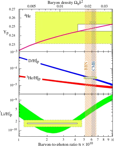
the calculation that are largely due to the uncertainty in the measurement of the neutron lifetime,τn= 885.7±0.8 s. For example, a ±0.16% uncertainty in the BBN calculation of

Yp can be derived from a ±2 s uncertainty in the neutron lifetime.

1.4.3 Limiting the Standard Model

The Standard Model includes Nν = 3 massless neutrinos. It has recently been

shown experimentally that an extension must be added to the Standard Model to account for a small neutrino mass and a right handed partner as the measured ﬂavor oscillation between neutrino species requires (see Eqn. (1.49)). One proposed remedy is the addition

3_He/H_p 4_He

2 3 4 5 6 7 8 9 10

1

0.01 0.02 0.03 0.005

CMB

BBN

Baryon-to-photon ratio η × 1010 Baryon density Ω_bh2

D ___

H 0.24

0.23 0.25 0.26 0.27

10−4 10−3

10−5

10−9

10−10 2 5

7_Li/H p

Yp

D/H p

Figure 1.5: Calculation of light element abundances as a function of baryon-photon ratio,

η, bands represent the 95% CL. The observed values are shown in boxes (smaller boxes:

(38)

small mass. The addition of such a species will not aﬀect the establishedNν = 2.92±0.05

[18] from the invisible Z width measured in e−e+ colliders that represents a number of

SU(2)L doublet neutrinos.

Additional neutrino species are not easily detectable through conventional meth-ods of measuring weakly interacting species. However, if they maintain a coupling to the universe (i.e. via gravitational interactions, etc.) during the epoch of the n/p decoupling, they will boost the relativistic energy density and therefore the expansion rate of the uni-verse. This will extend the freeze-out to occur at a lower temperature, resulting in an increase in the abundance of4_{He in the early universe. Using known abundances, a bound} can therefore be set on the number of neutrino species[38][39][40],

Nν = 3 +fB,F

X

i

gi

2

Ti

Tν 4

. (1.81)

Here gi are the number of weakly interacting helicity states, fB = 8/7 (bosons) and fF =

1 (fermions). The situation is further complicated by the matter-enhanced mixings of the sterile neutrino with the left-handed doublets and thereby equilibrating Ti/Tν ≃ 1.

Additionally such mixings can produce νe, ¯νe asymmetries that modify the interconversion

of neutrons and protons, further modifying the 4He abundance. Using aχ2 ﬁt to minimize uncertainties from both the BBN calculated and measured values of the abundances Y4,2,7 a limit of 2< Nν <4 can be set[39].

1.5 Summary

Theories included in the Standard Model of particle physics have been very suc-cessful. They have accurately described the weak interactions in terms of anSU(2)_⊗U(1) gauge theory. This includes a quantitative description of β-decay, and can thus be further used as a probe for additions to the Standard model such as new quark generations.

Similarly, the Big Bang Nucleosynthesis model is a highly successful model of the early universe. It accurately predicts abundances of light nuclei that span eight orders of magnitude. A more precise measurement of the neutron lifetime may allow the theory to provide even more predictive potential in areas such as the number of neutrino ﬂavors.

(39)

Chapter 2

Neutron Lifetime Measurement

Techniques

2.1 Neutron Sources

The lifetime of the neutron is short on the scale of the life of a typical observer, but long on the scale of nuclear processes. Therefore, there are no natural sources of free neutrons available with a sufficient density such that the number of decays are statistically significant for studies. The majority of neutrons in the universe are bound within nuclei, and thus to create a source one must liberate them from the nuclei. Two types of laboratory neutron sources commonly used for research are reactors and spallation sources. Through fission processes, reactors can provide useful quantities of neutrons for study. Secondly, when high energy particles are incident on heavy nuclei, the nuclei will fission, and one of the fragmentation products are neutrons.

Just as we classify the different types of electromagnetic radiation by wavelength or energy, so too can one classify neutron radiation. There are no distinct boundaries between the classifications, rather there are rough guidelines highlighting the boundaries between the classes of neutron energies. Neutrons freed from nuclei via fission processes are known as fast neutrons. These are neutrons with energies of_∼1 MeV, corresponding to velocities of 14,000 km/s.

(40)

N

e

u

tr

o

n

E

n

e

rg

y

(

e

V

) Neutr

on V

elocit

y (m/s)

Figure 2.1: Typical neutron energies span many orders of magnitude. As described in Chapter 3, neutrons entering the experimental cell have a peak energy near 1 meV and are subsequently downscattered in liquid helium to energies below 240 neV.

moderator are said to have been thermalized when they have reached equilibrium with the moderator. For room temperature moderators surrounding the source this corresponds to

kB·300 K, or 25.85 meV, orvth = 2224 m/s, where kB is the Boltzmann constant. Those

neutrons not fully thermalized by the room temperature moderator are known as epithermal neutrons.

(41)

2.2 Properties of Ultracold Neutrons

At very low energies the neutron’s wavelength is long enough that it samples many nuclei when it approaches a material surface. The neutron wavefunction can be represented by an incident wave and the sum of spherical scattered waves from the individual nuclei. As a consequence of the diﬀerence in scales between the neutron wavelength and the density of nuclear scatterers, the strong nuclear force may be represented as an eﬀective nuclear pseudo-potential[41],

V = 2π~ 2

mn

X

i

Niai. (2.1)

A linear combination of the nuclear number density,Ni, and the coherent neutron scattering

length, ai, of the full stoichiometry of the material, where mn is the neutron mass.

Since V is typically the same order of magnitude as cold neutrons, they may be reﬂected from surfaces at angles less than the critical angle (see Eqn. (1.2)). Similar to light transport through ﬁber optics, neutron scattering facilities utilize this property transporting neutrons long distances via neutron guides.

When neutron energies are sufficiently low such that their energies are equal to or lower than the material wall potential, total internal reflection occurs at normal incidence. Such neutrons are classified as ultracold (UCN) with kinetic energies of 300 neV or less. As such, UCN are slow moving particles. They have a maximum velocity of _∼7.6 m/s and travel on parabolic trajectories. UCN interact with gravity converting kinetic energy to potential energy at the level of 102 neV/m. The neutron is a neutral particle and to first order does not interact with electric fields. However, its small magnetic moment does interact with a magnetic field at the level of 60 neV/T. Therefore, an ultracold neutron is a class of particles that experience magnetic, gravitation, and nuclear forces with comparable strengths.

2.3 Neutron Beta-Decay

(42)

Measurement Year Measurement Year

Neu

tr

o

n

L

if

et

im

e (

s)

Neu

tr

o

n

L

if

et

im

e (

s)

1940 1950 1960 1970 1980 1990 2000 2010 1600

1400

1200

1000

800

PDG average

Beam

Material Bottle

Material Bottle, Serebrov '05

Figure 2.2: a.) A timeline of all neutron lifetime measurements[42], b.) A closer view of the 7 measurements included in the PDG average, as well as a recent measurement by Serebrov et al. that was not included in this average[43].

(43)

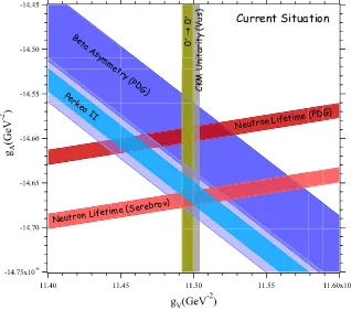
does however reiterate the need for additional measurements with similar precision to solve this discrepancy.

To understand how such a discrepancy eﬀects the unitarity of the CKM matrix, one can create exclusion plots from the diﬀering dependencies on the coupling constants using the most precisely determined decay correlation, the spin-electron correlation A, and the neutron lifetime. The value of A provides λ = ga/gv, while τn−1 ∝ (ga2+ 3gv2). This

exclusion plot is shown in Figure 2.3.

The PDG values of λ and τn are consistent, albeit with large error bars, with

the more precise determination of gv from both measurements of superallowed 0+ → 0+

nuclear beta decays and measurements of Vus and Vub when combined with the condition

that the CKM matrix is unitary. The newτnmeasurement [44] deviates from both of these

limits. Additionally a new measurement of theAcorrelation coeﬃcient by the Perkeo group in Heidelberg also modiﬁes the limits of gv away from those of the nuclear β-decays and

unitarity requirements[45]. It is interesting to note that the combination of both new values returns the agreement with the 0+_→ 0+ CKM unitarity limits.

A global analysis of neutron and nuclear decays further demonstrates the need to quantitatively address the discrepancies. The work of Severijns et al.[46] presents an analysis of the current situation in neutron and nuclear β-decay physics by relaxing the

V ₋A constraints toward the general Hamiltonian for β-decays presented by Jackson et al.[28] The authors have computed several ﬁts to all physically relevant data using several models of varying generality.

In the standard V ₋Aone-parameter ﬁt to λ, Severijns et al. computed a

χ2 _{= 74}_._{08 for the 25 degrees of freedom resulting in} _λ₌₋₁_._{27293(46). This fit includes} the most recent published value of the neutron lifetime[44]. If this value is excluded the χ2 for the fit is reduced to 25.86 for 24 degrees of freedom, and the resultingλ=₋1.26992(69). If the V ₋A assumption is relaxed to allow for scalar and tensor couplings through a fit to three free parameters, CA/CV,CS/CV, andCT/CA, the addition of the Serebrov value

of the neutron lifetime leads to a non-zero tensor component, CT/CA= 0.0086(31), albeit