Improved Internal Relief Valve Performance Through Study Of Reduced Cracking To Full By-Pass Pressure Using CFD Simulation

(1)

University of Windsor University of Windsor

Scholarship at UWindsor

Electronic Theses and Dissertations Theses, Dissertations, and Major Papers

7-11-2015

Improved Internal Relief Valve Performance Through Study Of

Reduced Cracking To Full By-Pass Pressure Using CFD Simulation

Yohance Bakari Henry

University of Windsor

Follow this and additional works at: https://scholar.uwindsor.ca/etd

Recommended Citation Recommended Citation

Henry, Yohance Bakari, "Improved Internal Relief Valve Performance Through Study Of Reduced Cracking To Full By-Pass Pressure Using CFD Simulation" (2015). Electronic Theses and Dissertations. 5325. https://scholar.uwindsor.ca/etd/5325

This online database contains the full-text of PhD dissertations and Masters’ theses of University of Windsor students from 1954 forward. These documents are made available for personal study and research purposes only, in accordance with the Canadian Copyright Act and the Creative Commons license—CC BY-NC-ND (Attribution, Non-Commercial, No Derivative Works). Under this license, works must always be attributed to the copyright holder (original author), cannot be used for any commercial purposes, and may not be altered. Any other use would require the permission of the copyright holder. Students may inquire about withdrawing their dissertation and/or thesis from this database. For additional inquiries, please contact the repository administrator via email

(2)

IMPROVED INTERNAL RELIEF VALVE

PERFORMANCE THROUGH STUDY OF REDUCED

CRACKING TO FULL BY-PASS PRESSURE USING CFD

SIMULATION

By

YOHANCE HENRY, M.Eng., P.Eng.

A Thesis

Submitted to the Faculty of Graduate Studies

through the Department of Mechanical, Automotive & Materials Engineering in Partial Fulfillment of the Requirements for

the Degree of Master of Applied Science at the University of Windsor

Windsor, Ontario, Canada 2015

(3)

IMPROVED INTERNAL RELIEF VALVE

PERFORMANCE THROUGH STUDY OF REDUCED

CRACKING TO FULL BY-PASS PRESSURE USING CFD

SIMULATION

by

Yohance Henry, M.Eng., P.Eng.

APPROVED BY:

______________________________________________ Dr. N. Biswas

Department of Civil and Environmental Engineering

______________________________________________ Dr. G.W. Rankin

Department of Mechanical, Automotive and Materials Engineering

______________________________________________ Dr. R.M. Barron, Co-Advisor

_____________________________________________________ Dr. R. Balachandar, Co-Advisor

(4)

iii

DECLARATION OF ORIGINALITY

I hereby certify that I am the sole author of this thesis and that no part of this thesis has been published or submitted for publication.

I certify that, to the best of my knowledge, my thesis does not infringe upon anyone’s copyright nor violate any proprietary rights and that any ideas, techniques, quotations, or any other material from the work of other people

included in my thesis, published or otherwise, are fully acknowledged in accordance with the standard referencing practices. Furthermore, to the extent that

I have included copyrighted material that surpasses the bounds of fair dealing within the meaning of the Canada Copyright Act, I certify that I have obtained a written permission from the copyright owner(s) to include such material(s) in my

thesis and have included copies of such copyright clearances in my appendix. I declare that this is a true copy of my thesis, including any final revisions,

(5)

iv

ABSTRACT

Relief valves are widely used in the process industry. Their ultimate role is to

mitigate adverse conditions that would jeopardize safety and incur catastrophic losses, especially with respect to human life. The primary focus of this research is to investigate the performance of relief valves, with the specific objective of

reducing the cracking to full by-pass pressure in internal relief valves of positive displacement pumps. Two and three-dimensional computational fluid dynamics (CFD) models of an external relief valve are developed and used to evaluate the

effects of the mesh, numerical parameters and boundary conditions on the results, including flow pressure and velocity field. Knowledge gained from the external

relief valve study has guided the internal relief valve simulations, particularly with regards to sensitivity of the results to the mesh and other numerical settings. Numerical simulations were performed utilizing the CFD codes: ANSYS Fluent

(6)

v

DEDICATION

To my wife Keisha Henry and our three wonderful boys Yohance Jr., Djimon and Ajani Henry

also

(7)

vi

ACKNOWLEDGEMENTS

This research is industry based through the company-Viking Pump Inc./Viking

Pump of Canada. I would like to thank Jim Mayer, Brian Comiskey, Patrick Taylor, Joe Thompson, Tony Dutcher, Mike Ramsey, Derrick Goddard, Joe Toy, Wayne Fortin and Chris Nantau, a combination of upper management and department

specific employees. They all contributed to my Thesis, by sharing their knowledge of the Internal Relief Valve being researched.

I would like to express my sincere thank you to my advisors: Dr. Barron

and Dr. Balachandar, for their continuous support, knowledge and valued input to my thesis work. Without their patience, resilience and understanding of the

difficulties of this research, I would not have been able to successfully complete it. I would also like to thank all my colleagues: Kohei Fukuda, Sudharsan Balasubramanian, Abbas Ghasemi, and Mehrdad Shademan, for their time,

consideration and knowledge that they shared during my research, especially Kohei Fukuda for lending his great input with respect to CFD modeling.

I would also like to extend my thank you to all faculty and staff members of the Department of Mechanical, Automotive and Materials Engineering and

(8)

vii

LIST OF TABLES

(11)

x

LIST OF FIGURES

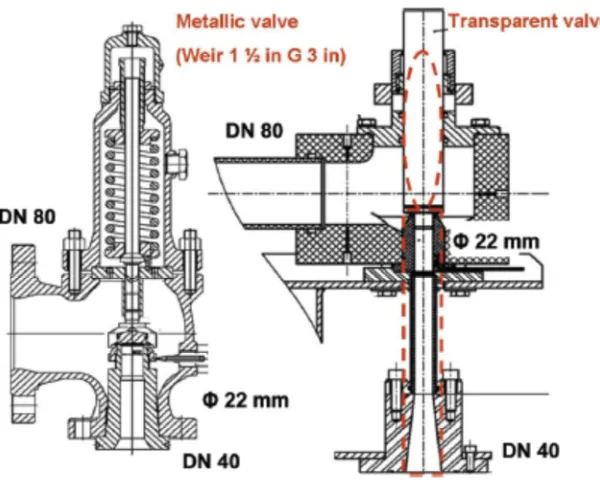
Fig. 2.1: Comparison of metallic and transparent valves ……….6

Fig. 2.2: Transparent valve used by Kourakos et al. [2]………...7

Fig. 2.3: Fig. 2.3: Metallic valve used by Kourakos et al. [2]...7

Fig. 2.4: Axisymmetric grid of metallic ERV for CFD simulations……….9

Fig. 3.1: Internal gear pump operation………17

Fig. 3.2: Internal gear pump with IRV mounted on top………..18

Fig. 3.3: Cutaway of Viking internal pressure relief valve……….19

Fig. 3.4: Detailed view of nozzle - valve disc……….20

Fig. 4.1: General design of a spring operated safety relief valve………23

Fig. 4.2: Clustered mesh with boundary conditions………....24

Fig. 4.3: Scaled residuals (Case A)……….26

Fig. 4.4: Contours of velocity magnitude (Case A)………27

Fig. 4.5: Contours of static pressure (Case A)………28

Fig. 4.6: Contours of dynamic pressure (Case A)………...28

Fig. 4.7: Re-designed ERV model with multi-block mesh (Case B)………..29

Fig. 4.8: Discharge nozzle extensions...………30, 46 Fig. 4.9: Scaled residuals (Case B)……….30

Fig. 4.10: Contours of velocity magnitude (Case B - 101.6 mm extension)……...31

Fig. 4.11: Comparison of velocity magnitude contours (Cases B and D)………...33

Fig. 4.12: Streamlines coloured by velocity magnitude (Cases B and C)………...35

Fig. 4.13: Y+on disc walls………...36

(12)

xi

Fig. 4.15: Check for back flow in the discharge line………..38

Fig. 4.16: Check for back flow in the discharge line………..39

Fig. 4.17: Pressure inlet/outlet BC’s vs inlet/outlet BC’s (Cases C and F)……….41

Fig. 4.18: Schematic of divergent-convergent model, incorrectly depicting an ERV……….43

Fig. 4.19: Schematic of convergent-divergent nozzle, correctly depicting a valve analogous to an ERV………..44

Fig. 4.20: Velocity magnitude contours (Cases G and H)……….…..45

Fig. 4.21: Outlet condition check – velocity vectors………...47

Fig. 4.22: Outlet condition check – dynamic pressure profiles………...48

Fig. 4.23: Mesh of 3D ERV………49

Fig. 4.24: Dynamic pressure contours of 3D Valve………....50

Fig. 5.1: Viking safety relief valve performance curve (K-LS size pump)……….52

Fig. 5.2: Relationship between cracking and full by-pass pressure ………...54

Fig. 5.3: Cross-section of the 3-795 series Viking IRV ……….………56

Fig. 5.4: 3D mathematical representation of 3-795 series IRV………...56

Fig. 5.5: Cross section of 3-795 series IRV………..57

Fig. 5.6: Cross-sections of complete IRV and modeled IRV with interior wetted surfaces……….58

Fig. 5.7: Poppet original and offset distance, 3D offset distance shown as well…59 Fig. 5.8: Surface and volume mesh……….61

Fig. 5.9: Performance curve - IRV set pressure setting = 565 kPa (82 psi)………64

(13)

xii

Fig. 5.11: Residuals for k-ω_{turbulence model (1}st_{-order upwind)……….66}

Fig. 5.12: IRV – Assembly clearance………..67 Fig. 5.13: Velocity vectors, coloured by velocity magnitude – k-ε_turbulence

model; 1st-order upwind scheme………68

Fig. 5.14: Velocity vectors, coloured by velocity magnitude – k-ω_turbulence

model; 1st-order upwind scheme………69

Fig. 5.15: Residuals for k-ε_{turbulence model (2}nd_{-order upwind)………..70}

Fig. 5.16: Residuals for k-ω_{turbulence model (2}nd_{-order upwind)………70}

Fig. 5.17: Velocity vectors, coloured by velocity magnitude – k-ω_turbulence

model; 2nd-order upwind scheme………...71

Fig. 5.18: Velocity magnitude contours – k-ω_{turbulence model;}

2nd-order upwind………....72

Fig. 5.19: Velocity magnitude contours and streamlines – k-ω_{turbulence model;}

2nd-order upwind scheme……….73

Fig. 5.20: Total absolute pressure – k-ω_{turbulence model; 2}nd_{-order upwind}

Scheme………...74

Fig. 5.21: Wall Y+ of IRV shell –k-ω_{turbulence model;}

2nd-order upwind scheme.………...74

Fig. 5.22: Wall Y+ of IRV cross-section (near-wall)………..75

(14)

xiii

Fig. 6.2: Added features for better flow distribution…...………...80

Fig. 6.3: Removal of assembly clearance and wall thickness……….81

Fig. 6.4: Adding convex curvature to front face of poppet and

(15)

xiv

LIST OF APPENDICES

APPENDIX A - Copyright Permission Documents

Figure A.1 – Permission for use of Viking Pump Inc. relief valve in thesis...88

Figure A.2 – Permission for use of Viking Pump figures in thesis [8], [9], [11]....89

Figure A.3 – Permission for use of figures 1, 2, 4 and 6 in reference [2]………...92

Figure A.4 – Permission for use of one figure on page 85 in reference [10]…...93

APPENDIX B - Calculations

Figure B.1 – Divergent-convergent model (3D), incorrectly depicting an ERV....94 Figure B.2 – Convergent-divergent nozzle (3D), correctly depicting a valve

(16)

xv

LIST OF ABBRREVIATIONS/SYMBOLS

ACSL Advanced Continuous Simulation Language

API American Petroleum Institute

ASME American Society of Mechanical Engineers CFD Computational fluid dynamics

CPRV Charge pressure relief valve ERV External relief valve

IRV Internal relief valve PMMA Polymethyl methacrylate

NPSHa Net positive suction head available

NPSHr Net positive suction head required NSE Navier-Stokes equation

(17)

xvi

NOMENCLATURE

k Kinetic energy of turbulence

ε _{Dissipation rate of turbulence}

ω _{Dissipation rate of turbulence (turbulent frequency)}

Cb Correction coefficient

CD Drag coefficient

(18)

1

CHAPTER 1. INTRODUCTION

Internal relief valves (IRV) are mounted as over-pressure protection devices on internal gear pumps. The IRV’s main role is to reduce the pressure if an over-pressure

situation occurs. The IRV can be viewed as a robust safety feature, but most internal/external gear pumps do not have them as part of a standard design. This is due to

a combination of cost and design criteria needed to implement the IRV on the gear pump. Very little research has been done towards improving the IRV’s performance. The IRV design specifically related to Viking Pump Inc. has been in existence for over 100 years

with very little change to the design. The major hurdles with researching these components are mainly the accessibility in viewing the flow pattern and understanding

how the flow pattern changes if components are modified within the IRV.

Internal gear pumps are a positive displacement pump, which means that the discharge head vs. flow characteristic is vertical, thus the flow is inherently independent

of the discharge head. Liquid is rotated from suction to discharge through cavities within the gear teeth and casing. If there is a blockage on the discharge side of the pump, such as

a valve being closed in the discharge line, there will be an immediate pressure build-up. This pressure build-up could be catastrophic if it is not mitigated immediately or at least within a suitable time. If this occurs, the pump will fail internally, or the motor will stall,

or the drive equipment will fail, or the process piping will fail catastrophically. It is because of these potential failures and the severe consequences that it is imperative that

some form of over-pressure protection be used in internal gear pump arrangements. This protection could be through the use of an internal relief valve, an external relief valve, a

(19)

2

There is great interest in improving the relief valve performance of internal gear pumps. There are many key advantages related to internal gear pumps that could be

gained from research carried out towards improving the IRV performance. These improvements could help pump companies be more competitive from an applications standpoint by reducing the customers’ operating costs while improving safety. A detailed

understanding of the liquid flow inside the IRV will also help to design more efficient internal gear pumps for applications involving thin liquids operating at high pressures.

Further details with regard to potential improvements will be discussed later in this thesis.

The internal relief valve is composed of three main components, the poppet, spring and adjusting screw. These three components are essential for setting the cracking

pressure (pressure at which the IRV begins to open) at which the poppet begins to lift, forming an orifice with the seat while pushing against the spring to create full by-pass in

an over-pressure situation. The concepts behind this full operation will be highlighted and explained later in this thesis.

A preliminary computational fluid dynamics (CFD) study was first performed on

a simple model of an external RV, primarily to get a feel for the main characteristics of the flow fields associated with RVs, such as: the pressure field, velocity field, regions of separation and flow streamlines. This exercise included preliminary validation of the

numerical models and the opportunity to become more familiar with the software and how results are affected by different parameter settings. Based on the experiences gained

(20)

3 The main goals/motivation of this thesis are:

1. to understand how CFD can be leveraged, in lieu of the availability of physical hardware and instrumentation typically reserved for laboratory research simulations;

2. to optimize the parameters that favour a reduced range of cracking to full by-pass pressure in internal and external relief valves and therefore improve their

(21)

4

CHAPTER 2. LITERATURE REVIEW

2.1. Introduction

Several journal articles, papers and reports produced by valve companies were reviewed to evaluate the performance status of relief valves. No research exists with

respect to internal relief valves. The following review of the available literature, however, highlights those results which offer some guidance and reflections on the goals of this

thesis.

2.2. Previous Studies Related to Internal/External Relief Valves

Mayer et al. [1] conducted a study to obtain information on the operation of the Viking Pump IRV. The main characteristics studied involved flow vs. pressure as well as

poppet lift (calculated and measured). The information obtained from the study was used to develop the governing mathematical equations and a FORTRAN computer program to model the flow through internal relief valves.

The steady-state flow force equation, spring force and drag force on poppet were used in the force analysis of the poppet. Drag coefficient (CD), discharge coefficient (Cd)

and velocity coefficient (Cv) were determined from performance tests and poppet lift measurements. From this analysis, the equation and computer program that was used to determine the flow area for a given poppet lift, poppet seat angle and poppet diameter

was highlighted. Graphical relationships of poppet lift (measured and calculated) and capacity vs. discharge were developed to predict relief valve performance at various

(22)

5

For specific relief valves in operation while the pump was running at speeds in the 500 RPM to 1200 RPM range, it was noted that the calculated and measured poppet lift

exhibited the same approximate relationship. These findings were documented in Viking’s Pump Internal Archive W.O. 4592 [1].

Kourakos et al. [2] investigated the external relief valve (ERV). The main focus

of their investigation was to determine the forces imposed on the valve disc for different inlet pressures and different disc positions using both experimental and CFD results.

They used a 40 mm (1.5 in.) ERV for the experimental setup. The ERV was modified by removing the spring. A force measuring device was mounted on top of the valve. With this experimental setup, they determined the forces applied on the disc at different inlet

pressures and disc positions. For each iteration, the disc was set at a new lift position (static position). Chosen set pressures and valve lift from preliminary dynamic valve

operation investigations were provided to analyze the forces imposed on the disc.

The experimental apparatus consisted of two ERV models, viz. a metallic model and a transparent model made of polymethyl methacrylate (PMMA), with slight design

differences. The metallic ERV model was used to analyze incompressible flow while the transparent model was used to analyze compressible flow. One notable difference

between the two models is that the plastic model had a longer inlet nozzle when compared to the actual metallic ERV. Another important difference was the ability for the original metallic ERV to handle higher pressures. The differences between these valves

(23)

6

Fig. 2.1: Comparison of metallic and transparent valves

(from Kourakos et al. [2], by permission of ASME)

Having a transparent valve allowed for complete optical visualization and

observation of the flow through the valve as well as cavitation and two-phase flow. Kourakos et al. [2] studied these effects in compressible and incompressible environments. Further highlights of how Kourakos et al. [2] analyzed the transparent and

(24)

7

Fig. 2.2: Transparent valve used by Kourakos et al. [2]

(by permission of ASME)

Fig. 2.3: Metallic valve used by Kourakos et al. [2] (by permission of ASME)

In the experimental setup involving the metallic valve, the back pressure affects

how the valve disc behaves. In the transparent model several pressure sensors were placed inside the valve. These allow for measurements of static pressure. In addition to measuring pressure inside the valve, additional pressure sensors were placed directly on

(25)

8

model is able to handle higher pressures compared to the transparent model. However, there is limited optical access with the metallic model and only the set pressure and back

pressure can be measured with this model.

Since our interest in the current research is to study the flow of water through a RV, only the incompressible environment of Kourakos et al. [2] will be discussed further.

In the experimental setup shown in Fig. 2.4, the metallic ERV is analyzed using water at ambient temperature as the test fluid. The calming reservoir is connected to a pump

capable of producing pressure up to 78 bars (1146 psi) and 250 m3/hr (1101 gpm) flow rate. The admission valve acts like a variable frequency drive (VFD) to control the flow entering the calming reservoir which leads to the long pipe connected to the test ERV.

The admission valve admits a certain percentage of flow into the calming reservoir. The author suggest that this is analogous to a variable frequency drive as it also acts as a flow

control device by reducing the motor speed of the pump which will only allow a certain percentage of the flow to leave the pump going into the process. Pressure on the free surface of the reservoir is fixed by compressed air. The flow rate entering the ERV is

measured by a flow meter. To obtain the best efficiency of the pump, the discharge valve operates as a by-pass. This setup permits the observation of opening pressure, closing

pressure and the discharge coefficient. Also, the approximate flow force on the disc is acquired as well with sensors mounted on top of the valve. The flow conditions analyzed in the ERV test setup are Pset = 0.7 - 11.0 bar (10.2-160 psi) and lift values at 0.5 to 7.2

mm (0.02 to 0.283 in.)

Computational Fluid Dynamics (CFD) simulations of the test ERV were also

(26)

9

for the simulations, with a 2D axisymmetric grid as shown in Fig. 2.4. The grid, which contained 1.45 x 106 cells, was designed with a particular focus on the disc region since

the primary interest was to determine the flow force on the disc. A steady-state case was assumed and the k-ω_{turbulence model was used with a second order discretization}

scheme. The pressure based solver of Fluent (pressure-velocity coupling) was used. The following set pressures and lift values were analyzed with the CFD model: Pset = 2, 3, 6 and 11 bar (29, 43.5, 87 and 159.5 psi) and lift values at 1.5, 3, 4.5 and 7.2 mm (0.06,

0.12, 0.18, 0.28 in.)

Fig. 2.4: Axisymmetric grid for the metallic ERV [2] (by permission of ASME)

To simplify the problem and to decrease computational time, the incompressible

flow was assumed to be steady and cavitation was neglected. From the CFD results, Kourakos et al. [2] concluded that the lowest lift produced the highest pressure concentration in the middle of the disc, whereas higher disk lift positions produced a

(27)

10

experimental and CFD results are compared, the measured and CFD computations provide reasonable predictions in flow force with CFD computations. Small deviations

existed between the tested and computational values. The adjustment ring location for the experiment created some experimental uncertainty.

The research conducted by Chabane et al. [3] concentrates on ERV’s subjected to

back pressure build up. They indicate that real world safety relief valves, having a back pressure that is 30% of the set pressure, generally use a balancing mechanism called a

bellows. The bellows helps to facilitate the reduction of the forces downstream, resulting in the balancing out of the downstream pressure. This helps to avoid vibration/chatter usually caused by back pressure. A poorly designed ERV can prove disastrous if back

pressure values are high. It is stated that a conventional ERV at 10% of the set pressure can be used without the balancing effects, however even with low values of back pressure

fluttering/chattering of the disc may still occur. Comparing the conventional ERV to the balanced bellows ERV, the balanced bellows ERV should be able to handle levels of back pressure in the vicinity of 40 - 50% of the set pressure, while maintaining its

approximate capacity.

Chabane et al. [3] looked at the ERV and the effects of back pressure from a

theoretical perspective. In theory, correction factors for back pressure can be obtained from the American Petroleum Institute (API) - API 520 Code. The code presents the correction coefficient (Cb) for back pressure values obtained from numerous ERV tests

(28)

11

effects caused by back pressure. According to the API 520 Code, experiments have shown that instabilities could occur with as little as 15% back pressure.

An experiment to evaluate this concept further was setup by Chabane et al. [3] using air with the ERV pressure set at 40 bar (580 psi). The air in the downstream reservoir was at 200 bar (2900 psi). Flow rates were measured using four Coriolis flow

meters. The flow meters were linked to a buffer tank where the ERVs were tested. Maximum pressure attainable was 40 bar (580 psi) and maximum mass flow rate was 13

kg/s (29 lb/s). The effects of pressure are detected when back pressure rises to about 10% of set pressure. When back pressure is higher, characteristics of the air flow change. Vibration and chattering occur when back pressure reaches values that are 25% to 30% of

set pressure.

A CFD model was also developed by Chabane et al. [3] for the numerical

simulation of the ERV and was validated with the experimental data. The CFX-11 code was used to solve the 3D Reynolds-Averaged Navier-Stokes equations. No symmetric considerations were assumed. A 3D unstructured mesh was used, comprised of

15,500,000 cells (3,000,000 nodes). Tetrahedral/prismatic elements were used close to the wall, at the nozzle and disc valve to ensure a Y+ value below 100. Unstructured

tetrahedral elements were used away from the walls. A steady flow approach was assumed, using the k-ε_{turbulence model with wall functions and 2}nd_{-order discretization} accuracy. Three cases were analyzed and compared to the experimental results; Case 1:

disc in almost closed position. Case 2: disc ½ way closed, and Case 3: disc at fully open position. Analysis of the flow patterns in these three cases confirms that the dynamics of

(29)

12

turbulence which causes load fluctuations. These fluctuations influence the movement of the blocking area (disc). Fluctuations also occur at lower disc lift. Due to stiffness of the

valve at smaller openings, the hydrodynamic forces vary between two and three times the value of the elastic force associated with the spring.

A thermodynamic model with test conditions was also developed by Chabane et

al. [3]. Due to compressibility of the air and gas the fast unsteady effects are normally considered insignificant and are not taken into account. Since there is a possibility that

equilibrium cannot reached due to pipe and control valve downstream creating back pressure, this could lead to chattering, which can be destructive to the safety valve depending on its frequency. This model was implemented to better understand the

dynamic behaviour during a test with and without back pressure. Equations of motion were developed to help understand these effects.

It was important to get an idea of how back pressure affects the ERV when at a certain percentage of the set pressure. In this Thesis the assumption is made that back pressure effects are accounted for in the calculation of the differential pressure. The pump

is sized at the differential pressure before the IRV setting is applied.

Follmer and Schnettler [4] proposed developing a series of new API ERVs by

investigating the fluid flow and looking into a new method to perform flow force measurements. They were able to analyze which components in contact with liquid could be removed or improved. This was done to implement a series of new API ERVs which

could meet industry certification standards.

With regards to approval testing, only combinations of flow force and spring

(30)

13

of measurement for flow force by API 526 Codes. This method permits the accurate evaluation of flow force readings over a large pressure range. Thus, forces on the disc can

be evaluated from the flow force for various opening and closing values. The following conditions have to be met. The interaction between flow force and spring force is essential. This will help to determine what type of spring characteristics are needed. Also

the flow coefficient needs to be large enough to stay within the +/-5% tolerance band while maintaining its consistency (constant) while subjected to a pressure of 1 bar (14.5

psi) and up.

Optimization of the components was carried out using gases, steam and liquids. The blow down ring was removed as it does not impact the flow physically. The blow

down ring is a component which controls how slowly and how fast the disc closes. The term blowdown defines the disc moving down to close. The position of the blowdown

ring will determine how slow or how fast the disc closes. Calculations (CFD) were performed for 3D compressible and incompressible flows. Based on the CFD analysis, which was confirmed experimentally, a special ERV was designed that provided a

proportional performance and consistent opening for 100 bar (1450 psi) pressure and hot

water at 265⁰C. This valve was designed to conform to all API 526 specifications along

with approvals by ASME. The valve also was improved and optimised to accommodate

equal flow geometry for liquids (incompressible), gases and steams and also incorporates the ability to handle two-phase flows if needed.

Bilanin and Teske [5] investigated spring-loaded safety ERVs. Their goal was to

(31)

14

from this model. Bilanin and Teske [5] implemented this model and developed the COUPLE predictive dynamic model to simulate flow through an ERV. The COUPLE

model was used to explain the test data of the ERV such as chatter, lift characteristics, etc. The COUPLE code incorporated the flow path of the valve by specifying spring rate and the ring settings. The valve models were validated through experiments.

Using CFD, the Navier-Stokes equations (NSE) were also used by Bilanin and Teske [5] to predict the flow field within the valve. The governing differential equations

used to model the flow field were the Reynolds-Averaged Navier-Stokes equations. A comparison of the Navier-Stokes solution and the predictions from the COUPLE code was performed. The NSE results replaced the experimental testing for validation purposes

with respect to the COUPLE code. Exit angle, mass flow through the valve, seat force reduction and stem force on lifted ERVs were compared at different valve stem positions.

Oravec [6] investigated pressure rise rate characteristics and flow force acting on a poppet in a charge pressure relief (CPRV). They are both direct acting poppet style relief valves, where in an over pressure situation the poppet is lifted and allows flow to

recirculate through the relief valve and back to the process or through the pump. The operation of the charge pressure relief valve is very similar to the internal relief valve.

However, it can also be used in the process line, unlike the IRV which can only be used directly on the pump. The CPRV was analyzed using CFD and subsequently verified with experimentation. Three stroke positions were considered with poppet lift values of 0.5

mm, 1.5 mm and 3 mm, while being subjected to a range of flow rates. ANSYS ICEM CFD was used with a combination of a hexahedral, tetrahedral and wedge mesh. Velocity

(32)

15

be steady and the fluid was taken to be incompressible (oil). Post-processing of the CFD results was completed using three strokes (lift values) and three flow rates. From this

data, a quadratic equation was used to solve for flow rate, highlighting the relationship between spring force and flow force. Graphs were generated from calculated points and trend lines were implemented to support the data points.

For validation purposes, an experimental setup of the CPRV was prepared. It is important to note that neither the CFD nor the experimental setup incorporated the

dynamic aspects. The CFD simulation was compared to the experimental simulation using flow rate and pressure drop across the CPRV [6].

Pressure vessels normally have spring-loaded safety valves (SLSV) in the event

of an over-pressure situation. Sethi and Lai [7] explored the dynamic behaviour of SLSVs. Generally, the forces acting on the moving parts of these valves are non-linear. A

differential equation model was developed to simulate the non-linear effects of the SLSV. This model was used to predict the valve response time. In solving these equations, the Advanced Continuous Simulation Language (ACSL) was used to facilitate solution of the

4th-order differential equations utilizing the Runge-Kutta method. Sample tests of the Farris 7000 valve were conducted to acquire pressure time history. The response to the

valve, related to the driving pressure, was illustrated graphically and compared to the simulated study. There was close agreement between the simulated and experimental data. In conclusion, the simulated results seemed to predict the actual results fairly well.

The articles reviewed above are mainly associated with the ERV. There is not much published literature on the IRV. One main difference between the IRV and ERV is

(33)

16

with the ERV. However, the flow fields are in general very similar and the operation in an over-pressure situation is identical when comparing the ERV to IRV. The similarity of

these concepts suggests a close relationship between the physics associated with ERVs and IRVs which has been exploited in this thesis.

The major research motivation in this thesis is to reduce the cracking to full by

(34)

17

CHAPTER 3. INTERNAL GEAR PUMP AND RELIEF VALVE

OPERATION

It is essential to understand the internal gear pump operation and how it relates to

relief valve operation. The pump operation is explained in this chapter, followed by a focus on the specifics behind the internal and external relief valve operation.

3.1. Internal Gear Pump Operation

The internal gear pump operates on a fairly simple concept. The term “positive

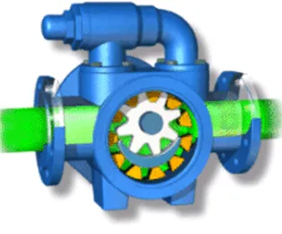
displacement” is a direct representation of how internal gear pumps operate. Referring to Fig. 3.1, at Step 1 the liquid enters the rotor and idler gear as the pump develops pressure.

The arrows indicate the direction of the flow. At Step 2 the liquid travels between the teeth of the rotor and idler gear teeth separately (gear within a gear principle). The moon shaped crescent helps to divide the liquid and acts as a seal between the suction and

discharge ports. At Step 3 the pump is nearly flooded and the gear teeth have a finite volume of fluid between them. In Step 4 the rotor and idler teeth are completely aligned

to form a seal. As the liquid now has nowhere else to go, it is forced out of the port into the discharge process line.

Fig. 3.1: Internal gear pump operation

(35)

18

3.2. Internal Relief Valve Operation

The IRV is the most important component on internal gear pumps with regards to safety. It is directly mounted on the pump and is the sole device that provides protection against over-pressure inside the pump. Figure 3.2 illustrates an IRV mounted on an

internal gear pump.

Fig. 3.2: Internal gear pump with IRV mounted on top

(from http://www.vikingpump.com [8], by permission of Viking Pump Inc.)

When an over-pressure situation occurs, the IRV allows the fluid to recirculate inside the pump until the pressure is brought down below the setpressure point. The

mechanism by which this occurs can be explained by referencing Fig. 3.3. The spring (A) holds the poppet in place. The poppet guide vanes rest on the internal wall of the IRV in

the valve body (C), while the spring (A) holds the poppet (B) against the valve seat. This position of the poppet is maintained by a force which is determined by the spring size as well as how tightly the spring is compressed by the adjusting screw (D). In an

(36)

19

exerted by the spring (set force or set pressure of the spring) and the poppet begins to lift. When the poppet lifts the liquid begins to flow through the IRV and return back into the

suction port of the pump. As the pressure keeps building up past the set pressure, all the liquid will eventually flow through the valve and back into the pump. At this point no

liquid will be leaving through pump discharge. This recirculation will continue until the force or pressure drops below the set force or pressure value at which the spring was originally set.

Fig. 3.3: Cutaway of Viking internal pressure relief valve [9]

(by permission of Viking Pump Inc.)

3.3. External Relief Valve Operation

(37)

20

Fig. 3.4: Detailed view of nozzle and valve disc [2]

(by permission of ASME)

The ERV operates on exactly the same principle as the IRV. When the spring force is overcome by the force of the liquid coming through the nozzle, the spring

compresses and the valve disc opens. The valve disc will not close until the force of the liquid drops below the spring force (set pressure of spring). It can be noted as well that the cross-sectional area of the valve disc (A2) is designed to be larger than that of the

nozzle (A1). For a constant system pressure, when the fluid exits the nozzle and enters a larger area the disc will experience a larger force that will prevail over the disc and thus

the spring force keeping the disc open. This could result in the valve subsequently opening too quickly. Flow velocity could cause changes in valve lift by changing the lift height. Due to this larger area, the valve disc will not close until the system pressure goes

(38)

21

in Fig. 3.4. Its geometry is one of the factors determining when the valve will close. The adjustment ring is used to control the opening or re-seating characteristics of the disc.

(39)

22

CHAPTER 4. CFD SIMULATION OF AN EXTERNAL RELIEF

VALVE

4.1. Introduction

As mentioned above, the external relief valve (ERV) exhibits flow features that

are similar to the internal relief valve (IRV), but the geometry of the ERV flow region is simpler than the IRV. In this research the ERV was used as a starting point to investigate meshing requirements, numerical parameter settings in the software and key features of

the flow field. Gambit and ANSYS Fluent [version 13] Computational Fluid Dynamics (CFD) software were used for mesh generation and to perform the CFD simulations,

respectively. A simplified ERV design was used to reduce difficulties associated with generation of the mesh. Both two-dimensional (2D) and three-dimensional (3D) ERV

simulations were carried out.

4.2. External Relief Valve (2D simulation)

A simplified 2D model of an external relief valve was utilized for the first stage of the CFD study. The simplified ERV model was developed by using a typical ERV as a reference, as shown in Fig. 4.1. The circled area of the ERV in Fig. 4.1 was used to

(40)

23

Fig. 4.1: General design of a spring operated safety relief valve (from Helleman [10], by permission of Elsevier)

The objective of this exercise was to model a flow field similar to, but less

complicated than the IRV. In doing so, the simplified 2D model of the ERV was used to determine appropriate settings that should be used for the 3D simulations of the ERV and

IRV. The simplified ERV analysis provides the necessary knowledge and tools needed to entertain the more complicated IRV design, which is the main focus of this thesis. Settings of particular interest are:

• turbulence model;

• type of upwinding, i.e., 1st or 2nd-order to achieve greater theoretical accuracy;

• the convergence criteria, which can be manipulated with a tighter tolerance band

to achieve better results;

• relaxation factors, which can be adjusted to help smooth out the oscillations of

(41)

24

With respect to the ERV model, certain assumptions were made to simplify the geometry and for the computational analysis. The ERV was initially modelled with a

simplified rectangular design as shown in Fig. 4.2. The diameters of the inlet and outlet were assumed to be the same. This was done to simulate the IRV, where the inlet and

outlet ports are the same size. The outlet was taken flush with the side wall.

The mesh employed for the ERV simulation was a structured quadrilateral mesh as shown in Fig. 4.2. Clustering was applied along the solid walls and at sharp corners to

capture boundary-layer effects and regions of flow separation. Cell aspect ratios ranged from 1.0 and 1.04.

Fig. 4.2: Clustered mesh with boundary conditions

An incompressible Newtonian fluid (water) with viscosity of 1 centipoise was

used in this analysis. The flow was taken to be steady, with an inlet velocity of 2.1 m/s (6.9 ft/s), approximately equivalent to 34 m3/hr (150 gpm). This is the typical flow rate

(42)

25

by-passed by a typical IRV during a complete by-pass situation. Fig. 4.2 also illustrates the boundary conditions that were implemented. It was further assumed that the ERV disc

would be at its maximum lift position of 76.2 mm (3 in.) in a complete by-pass situation. Turbulence intensity was set at 5% (medium turbulence). The hydraulic diameter was set to 76.2 mm (3 in.). The ERV walls were defined with no slip wall boundary conditions.

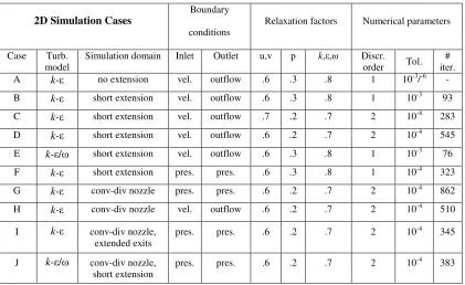
Several test cases were set up to evaluate the effect of the different settings of interest mentioned above. A summary of the main parameters in the simulations is

provided in Table 4.1.

2D Simulation Cases

Boundary

conditions

Relaxation factors Numerical parameters

Case Turb. model

Simulation domain Inlet Outlet u,v p k,ε,ω Discr. order Tol.

# iter. A k-ε no extension vel. outflow .6 .3 .8 1 10-3/-6 - B k-ε short extension vel. outflow .6 .3 .8 1 10-3 93 C k-ε short extension vel. outflow .7 .2 .7 2 10-4 283 D k-ε short extension vel. outflow .6 .2 .7 2 10-4 545 E k-ε_/ω short extension vel. outflow .6 .3 .8 1 10-3 ₇₆ F k-ε short extension pres. pres. .6 .3 .8 1 10-4 323 G k-ε conv-div nozzle pres. pres. .6 .2 .7 2 10-4 862 H k-ε conv-div nozzle vel. outflow .6 .2 .7 2 10-4 510

I k-ε _{conv-div nozzle,} extended exits

pres. pres. .6 .2 .7 2 10-4 345

J k-ε_/ω _{conv-div nozzle,} short extension

pres. pres. .6 .2 .7 2 10-4 383

Table 4.1: Test cases for 2D model of ERV

Case A: Initial simulations were performed using first order upwinding. The inlet

boundary conditions were set as a velocity inlet, with velocity of 2.1 m/s (6.9 ft/s). The outlet boundary condition was specified as outflow. The flow variables were initialized

(43)

26

convergence tolerance was set at 1.0x10-3 for the continuity and x- and y-momentum equations. The convergence tolerance for the turbulent kinetic energy and dissipation was

set at 1.0x10-6. These tolerances are the default values in ANSYS Fluent. The k-ε turbulence model with near-wall treatment was used since it gives fairly accurate results in the majority of uncomplicated fluid flows, and is the most popular model for industrial

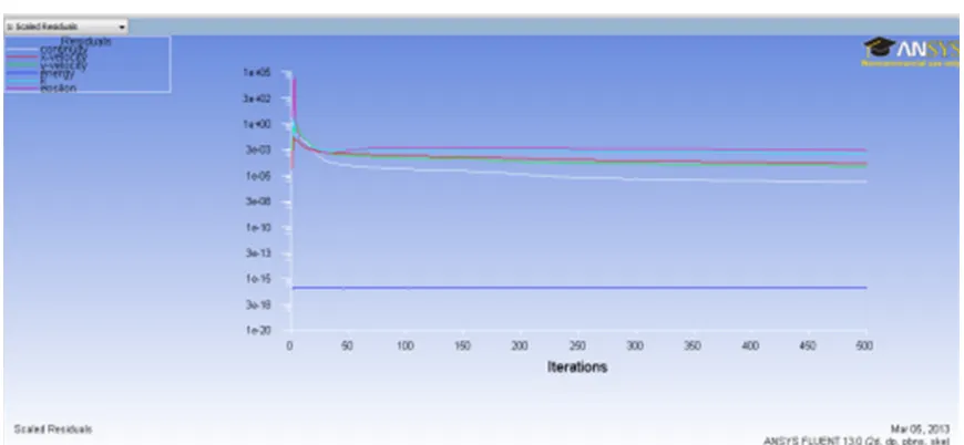
simulations. Under-relaxation factors are listed in Table 4.1. With these settings, the residuals stabilized after approximately 100 iterations, but did not fall below the specified

tolerance within 500 iterations, as seen in Fig. 4.3.

Fig. 4.3: Scaled residuals (Case A)

This simulation was initially carried out on a coarser mesh than shown in Fig. 4.2 and, although the solution did not converge, it suggested certain modifications to the

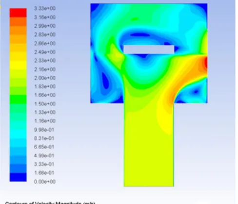
mesh. The mesh in Fig. 4.2 is the result of these modifications. The numerical set up was evaluated by examining: the contours of velocity magnitude; contours of the x- and y-components of velocity; velocity vectors and pressure contours. The velocity magnitude

(44)

27

valve. The acceleration of the fluid as it is deflected by the disc is also captured. However, this plot clearly suggests that the exiting flow is not aligned with the x-axis,

which is the fundamental assumption of the outflow boundary condition.

Fig. 4.4: Contours of velocity magnitude (Case A)

The static and dynamic pressure distributions, shown in Fig. 4.5 and Fig. 4.6 respectively, were also assessed. As expected, the static pressure is highest on the frontal

face of the disc. The contours in Fig. 4.6 show that the highest dynamic pressure occurs where the velocity is at its highest as it goes around the sharp corner before it exits the

(45)

28

Fig. 4.5: Contours of static pressure (Case A)

Fig. 4.6: Contours of dynamic pressure (Case A)

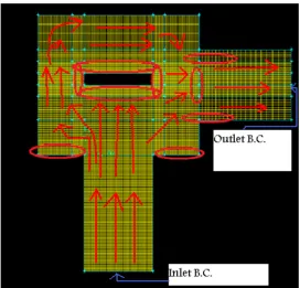
Case B: The analysis of case A indicates that there is a need to incorporate an outlet port on the discharge side of the valve to allow implementation of the outflow boundary

(46)

re-29

designed and the multi-block method was used to generate the mesh. A structured quadrilateral mesh was still utilized in this analysis. The re-designed ERV model is

shown in Fig. 4.7. The arrows schematically indicate flow direction and the elliptical curves identify regions where particular attention is required due to large gradients in the

flow variables.

Fig. 4.7: Re-designed ERV model with multi-block mesh (Case B)

If an outflow boundary condition is applied at the outlet, it is imperative that there is no back flow on the outlet plane. Therefore different outlet lengths, from 101.6 mm (4 in.) to 355.6 mm (14 in.), were investigated to determine the proper outlet length to

ensure a correct outflow condition was being investigated and to mitigate potential back flow. Schematics of the different nozzle lengths are illustrated in Fig. 4.8. For these

(47)

30

parameter settings in case A were retained, except that the tolerance for the turbulent kinetic energy and dissipation residuals was set at 1.0x10-3. For the domain with the short

discharge extension (101.6 mm), the solution converged in 93 iterations, as shown in Fig. 4.9. Other extended discharge lines also produced converged solutions.

Fig. 4.8: Discharge nozzle extensions

(48)

31

The velocity magnitude contours for the short extended nozzle are shown in Fig. 4.10. As the fluid enters the valve, some of the fluid particles accelerate to pass over the

sharp corner and move towards the discharge channel. Other fluid decelerates as it enters the larger valve region and encounters the disc. This flow behaviour is expected due to

the physical characteristics in the valve and the natural ability of the flow to take the path of least resistance.

Fig. 4.10: Contours of velocity magnitude (Case B - 101.6 mm extension)

Velocity vector plots and contours of turbulence (kinetic energy and dissipation),

turbulent intensity and static/dynamic pressure show that the change in valve geometry and mesh features using a multi-block method facilitate reduced computational time and improve accuracy in the CFD simulation. Although longer extensions to the discharge

(49)

32

negligible. Thus, the valve with the 101.6 mm discharge extension was retained for subsequent simulations.

Case C: Several parameters were changed to obtain more accurate results. The discretization of the convective terms was changed from first order upwind to second order upwind for momentum, turbulent kinetic energy and turbulent dissipation rate

equations. The relaxation factors for pressure, momentum and turbulent kinetic energy were changed as listed in Table 4.1. The convergence tolerances were also adjusted from

1.0x10-3 to 1.0x10-4 for continuity, x-velocity, y-velocity and turbulent parameters. The higher order upwinding and tighter tolerance produced more accurate results, with the

solution converging after 283 iterations.

Case D: To assess only the effect of under-relaxation factors, the momentum equations relaxation factor was reduced from 0.7 to 0.6 while others were kept the same as in case C. Under these conditions, the solution converged at 545 iterations. The solutions from

(50)

33 (Case B)

(Case D)

Fig. 4.11: Comparison of velocity magnitude contours (Cases B and D)

It can be observed that there is very little distinction in these contours in the region around the disc, although the discharge is modified. Pressure contours (dynamic and static) and velocity vectors were also compared for cases B and D (93 iteration

(51)

34

differences in these plots. Therefore it was concluded that these changes in the parameters did not make a significant difference.

Based on these preliminary investigations, it was decided to move forward with the following parameters, taking into account the desired accuracy and the computational time required for each simulation:

- convergence tolerances: 1.0 x10-4;

- relaxation factors: pressure = 0.2; default values for momentum, turbulent kinetic

energy, turbulent dissipation and turbulent viscosity;

- spatial discretization: second order upwinding for momentum, turbulent kinetic energy, turbulent dissipation; standard for gradient and pressure;

- turbulence model: k-ε_{with near-wall treatment.}

These parameters correspond to case C and yielded a solution after 283 iterations. The first order solution with tolerance 1.0x10-3 and convergence at 93 iterations and the

second order solution with tolerance 1.0x10-4 and convergence at 283 iterations are compared in Fig. 4.12. There appears to be no significant difference in the contours for

(52)

35 (Case B)

(Case C)

Fig. 4.12: Streamlines coloured by velocity magnitude (Cases B and C)

The wall Y+ value is usually used to determine whether the mesh is fine enough

(53)

36

bottom of the disc and increases from 30 to slightly above 50 on the side disc faces. The Y+ value at the top of the disc does not appear to be correct. The Y+ on the valve

boundary walls was also investigated and is illustrated in Fig. 4.14. Along the inlet section, the Y+ value ranges from slightly above zero at the entrance to almost 100 before

the fluid enters into the ERV body. The Y+ values on the ERV outer faces were also high, in the vicinity of 100 to 600. The separation, recirculation and reattachment occurring in the valve at these locations may be the cause of the high values of Y+. The

separation and recirculation make it more difficult to capture the boundary layer of the flow, where the velocity of the fluid increases from zero to some finite value across a

very short distance normal to the wall to form the boundary layer.

(54)

37

Fig. 4.14: Y+ on ERV boundary walls

(55)

38 (k-ε₎

(k-ω₎

Fig. 4.15: Streamlines coloured by velocity magnitude – k-ε_vs._k_-ω_{turbulence models}

Since the turbulence model has been changed, it is prudent to check the flow in the discharge section to ensure no back flow is present. To do this, five vertical

cross-sections were created in the outlet region of the ERV, as shown in Fig. 4.16. The velocity vectors on these vertical cross-sections were plotted and the findings show that near the

(56)

39

velocities) due to flow separation. However, at x = 9 the velocities are all positive giving a strong indication that no back flow is present near the exit of the outlet of the valve.

(a)

(b)

(57)

40

Case F: The velocity inlet and outflow outlet boundary conditions have been used in all the above simulations. However, it is important to check whether the velocity inlet

condition can be reproduced while imposing pressure inlet and pressure outlet conditions, since these are the type of boundary conditions that can be extracted for a typical industrial installation. A pressure inlet value of 2 kPa (0.3 psi) was estimated from the

velocity inlet profile and the dynamic pressure contours at the inlet. A pressure outlet condition was imposed at the outlet boundary and default values were used for the

various flow and numerical parameters except the tolerances which were set at 1.0x10-4. When comparing the velocity magnitude contours with case C, it was observed that the two sets of contours match fairly well, as demonstrated in Fig. 4.17. However, the

predicted velocity at the inlet was approximately 1.50 m/s (4.9 ft/s), which is less than original input value of 2.1 m/s used in Case C. Further investigation was conducted to

(58)

41 (Case C)

(Case F)

Fig. 4.17: Pressure inlet/outlet BC’s vs inlet/outlet BC’s (Cases C and F)

Case G: After further extensive investigation, it was apparent that the ERV should be viewed like a converging-diverging nozzle, where the seat and disc creates an orifice.

(59)

42

closed to a maximum, less than or equal to the inlet area, when fully opened. The valve geometry used in the above cases displays a divergent-convergent section. This indicates

that the orifice area, referred to as the throat or curtain area (area between bottom of the disc and the inlet nozzle seat), is larger than the inlet and outlet port areas. This completely defies the theory of valves. According to Bernoulli’s theorem, when a fluid

under pressure is accelerated through an orifice such as a valve, the static head is converted to the velocity head resulting in a pressure drop. If the area is smaller at the

inlet and outlet, the velocity will decrease as the flow enters the throat area. This could have an adverse effect on how the flow responds as it passes the valve throat, as shown in

(60)

43 (a)

(b)

Fig. 4.18: Schematic of divergent-convergent model, incorrectly depicting an ERV It would be beneficial if the throat or curtain area (orifice) were much smaller

than the inlet and outlet areas. To account for this, the curtain area has to be made smaller. This can be done by extending the valve nozzle seat as illustrated in Fig. 4.19. The distance between the bottom of the disc and the inlet into the ERV (curtain distance)

(61)

44 (a)

(b)

Fig. 4.19: Schematic of convergent-divergent nozzle, correctly depicting a valve analogous to an ERV

Following the same setup and procedure as in case F with the short extended outlet nozzle and using this new valve configuration which models the ERV as a convergent-divergent nozzle, the pressure inlet/outlet conditions reproduce the correct

(62)

45

Case H: The converging-diverging model that was used in case F was further investigated using velocity inlet and outflow boundary conditions, and the results are compared with

case F in Fig. 4.20.

(Case G)

(Case H)

(63)

46

Case I: With the new geometry it is necessary to check for possible back flow in the outlet nozzle and to see where the flow reattaches after it separates at the sharp corners in

the ERV. To verify that there is no backflow on the outlet plane, the discharge nozzle length was extended by 50.8 mm (2 in.), 127 mm (5in.) and 355.6 mm (14 in.), as shown in Fig. 4.8 and displayed below for convenience. However, the new configuration being

tested includes the curtain described above, which are not shown in Fig. 4.8.

Fig. 4.8: Discharge nozzle extensions

Pathlines, velocity magnitude contours and velocity vectors were plotted to determine where the recirculation occurs and where the flow reattaches. A vertical line

(64)

47

those shown Fig. 4.22 indicate that the recirculation and reattachment points are captured more effectively by extending the nozzle. However, this investigation was solely done to

ensure that no back flow was occurring and to determine if the outlet length of the valve needed to be longer to capture this feature. It was observed that by extending the discharge length, no back flow was present. This confirmed that the original outlet length

was adequate for further 2D and 3D analysis.

Determined their was

separation, thus back flow is occurring in nozzle

Extended nozzle an additional

14 inches which changed length to 18inches total

Re-attachment occurred at

approximately 9 to 10 inches in nozzle length

(65)

48

•

Does not capture recirculation

Does capture slight recirculation bubble

Dynamic pressure larger especially at 1.5 to 2” section of nozzle (Extended nozzle)-7000 Pa compared to 10000 Pa

Fig. 4.22: Outlet condition check – dynamic pressure profiles

Case J: The k-ε_{(standard and realizable) and} _k_-ω_{(standard) turbulent models were} investigated and compared using the new geometry described above. The results between

the models were not significantly different. However, for the 3D simulations, a model will be required that can handle adverse pressure gradients and give reasonably accurate

results with boundary layer flow. The k-ω_{turbulent model was selected for subsequent} simulations since the 3D ERV and the 3D IRV geometry (bends/corners/etc.) will be

more complicated.

4.3. Three-Dimensional Simulation of the ERV

A three dimensional model of the ERV was developed using the same parameters in Fluent with the k-ω_{turbulent model as in case J above. Figure 4.23 shows the hybrid} mesh that was used for the simulation, comprised of structured hexahedral and

(66)

49

cells. Dynamic pressure contours are shown in Fig. 4.24. This shows the surfaces on which the contours of dynamic pressure are plotted. Fig. 4.24 also displays a central

plane cross-section of the valve and shows that the high velocity fluid that is squeezed between the valve disc and the curtain contributes to the region of high dynamic pressure.

(67)

50 a)

b)

(68)

51

CHAPTER 5. INTERNAL RELIEF VALVE

5.1. Introduction

The internal relief valve (IRV) is a safety device which is essential in providing over-pressure protection to the internal gear pump. The IRV device not only protects the

pump from catastrophic failure but also serves as a protection measure for workers and the general public in the event of such a failure. In this chapter, a computational model

for the fluid flow through an IRV is developed and used to investigate the features of the flow through the valve at fully open condition. In particular, the CFD model provides detailed information on the velocity and pressure fields within the valve. Analysis of the

results leads to a fuller understanding of the valve operation and suggests potential modifications for improvement of the IRV.

5.2. Determining IRV pressure setting

The relationship between the internal gear pump and the IRV is based on the

differential pressure that the pump experiences and the capacity/flow that the pump produces. The IRV has a predetermined setting at which the valve will be fully open, thus

creating a full by–pass situation in the pump. In this scenario, the fluid will circulate within the pump and not leave through the discharge. The IRV setting is determined from an optimum point selected on a graph of the differential pressure vs. pump capacity, and

by a line intersecting the horizontal x-axis. For example, as shown in Fig. 5.1, the optimum point is generated by intersecting the pump capacity 14 m3/hr (60 gpm) and the

(69)

52

line on the graph. The full by-pass pressure is set at the point where this diagonal line intersects the horizontal axis. In practice, most pump internal relief valves are set at

approximately 172 kPa to 207 kPa (25 to 30 psi) above the differential pressure setting. However, the size of the pump, which influences capacity/flow capabilities, is often used as a measure to change this range to a higher value. It is important to note that the

differential pressure at which the pump is sized at is representative of the cracking pressure. Therefore in the example discussed above, 552 kPa (80 psi) which is the

differential pressure is the same value as the cracking pressure.

Fig. 5.1: Viking safety relief valve performance curve (K-LS size pump) [11]

(70)

53

5.3. Research Motivation

Advancement in product development is of utmost importance in the practical engineering world. Research plays a critical role in this type of engineering environment. In the present context, for companies like Viking Pumps Inc., exploring potential

techniques for improved IRV performance is key in moving forward with better products. The goal would be to reduce the range from cracking to full by-pass pressure of the IRV

as illustrated in Fig. 5.2. By achieving this goal, numerous direct benefits may be realized, as is further discussed.

To date very little is known about the poppet movement inside the internal

production relief valve. A couple of studies have been performed on prototypes for new designs, but these have not made it to production thus far. There have been no studies

done on production IRV’s to validate poppet movement. Once the IRV is subjected to an over-pressure situation, movement of the poppet cannot be confirmed precisely in a practical sense since the poppet is completely enclosed in the IRV. An experimental

study would require a transparent model and rather sophisticated measuring devices, thereby incurring considerable cost. A CFD analysis will provide detailed flow data from

(71)

54

Fig. 5.2: Relationship between cracking and full by-pass pressure [11]

(by permission of VikingPump Inc.)

By reducing the pressure range from cracking to full by-pass pressure, the fluid would by-pass earlier. This would lead to significant improvements in valve operation. It is anticipated that a reduction in the cracking to full by-pass range could be achieved by

modifying the IRV design, changing the functionality of a component, changing materials or through some other mechanism that improves the flow characteristics which

affect the forces acting on the poppet.