Article On the Noise Complexity in an Optical Motion Capture Facility

(1)

Article

On the Noise Complexity in an Optical Motion

Capture Facility

Przemysław Skurowski1* and Magdalena Pawlyta1,2

1

2

3

4

5

6

7

8

9

10

1 _Institute_of_Informatics,_Silesian_University_of_Technology,_Akademicka_16,_44-100_Gliwice,_Poland;

[email protected](P.S.);[email protected](M.P.)

2 _{Polish-Japanese}_Academy_of_Information_Technology,_Koszykowa_86,_02-008_Warsaw,_Poland;

[email protected]

* Correspondence:[email protected];Tel.:+48-32-2372151

Abstract: Optical motion capture systems are state-of-the-art in motion acquisition, however as

any measurement systemsthey arenoterrorfree – noiseis theirintrinsic feature. Theworks so

far mostly employ simple noise model, expressing the uncertainty as a simple variance. In the

workweprovetheexistenceofseveraltypesofnoiseanddemonstratehowtoquantifythemusing

Allanvariance. Fortheautomatedreadoutofthenoisecoefficientswesolvethemultidimensional

regressionproblemusingsophisticatedmetaheuristicsinexploration-exploitationscheme. Besides

classic types of noise weidentified thepresence of the correlated noises and periodic distortion

in ourfacility. We hadalso opportunity to observethe influenceof camerafailure tothe overall

performance.

Keywords: motion capture; evaluation; noise modelling; noise color; Allan variance; simulated

annealing;antcolonyoptimization

11

1. Introduction 12

Synthesis and analysis of human motion is an active research area having a plurality of

13

applications in biomechanics and entertainment. Contemporary technologies, allow to capture and

14

process the movement (Mocap) with high realism and accuracy, however, they are not error-proof.

15

Various methods were proposed for the motion acquisition, yet the optical motion capture (OMC)

16

technique, based on tracking of retro-reflective markers in IR images is considered as a gold standard

17

in this field of research. It outperforms other techniques and it has been used for verification of

18

the other technologies – inertial [1,2] or optical [3]. OMC is also considered as a reference motion

19

acquisition for the applications of other Mocap technologies in such demanding areas as medical

20

[4–6] or space research [7].

21

The uncertainty in optical motion capture systems depends on numerous factors, such as type

22

and amount of used cameras, their physical setup, and mounting, marker size, environmental

23

conditions such as air temperature or humidity, camera noise, and quality of the calibration of the

24

motion camera in the motion capture system. Though, almost all these factors can be controlled by

25

re-calibration of the system or ensuring constant environmental conditions, yet the noise present in

26

the cameras is an inevitable factor that cannot be easily neglected or removed.

27

In this article we characterize the types and levels of noise in three types of Vicon Motion

28

Capture Camera – MX-T40, Bonita10 and Vantage 5, we use Allan variance (AVAR) [8]n which

29

is a handy tool for identification and evaluation of noise types. We propose how to address the

30

non-trivial regression problem of ADEV curve, by matching it with the component functions using

31

(2)

metaheuristics – simulated annealing (SA) and ant colony optimization (ACO). Moreover, thanks

32

to the observed malfunction of one of the devices we were able to demonstrate, that the proposed

33

approach can be used for quite complex cases of correlated and periodic distortions.

34

The article is organized as follows – in the p. 2 we provide theoretical background and we

35

demonstrate, that simple variance-based noise quantification is not enough and we introduce Allan

36

variance as an alternative; in p. 3we describe experimental part – laboratory setup and procedure,

37

next it is followed with an algorithm for parameters estimation description and comments on

38

unexpected phenomena observed during the experiment; p.4discloses the experimental results and

39

their analysis followed by a discussion of results ; p.5summarizes the article and provides ideas for

40

future work.

41

2. Background 42

2.1. Previous works 43

The accuracy and precision in different OMCs were subject to analysis in several works [9–12]. In

44

those works, the most frequently studied OMCs are one of Vicon System (MX, Bonita, and V-series),

45

or OptiTrack system. Regardless of the system used, the authors of these studies agree that the

46

most important factor that influences the data is camera calibration. Camera calibration originates

47

from photogrammetry [13], it relies on positioning the cameras in a virtual 3D space so that they

48

correspond to the cameras positions in the laboratory. This position and several (minimum two)

49

2D camera projections of markers are used to reconstruct markers in 3D space [14]. The calibration

50

quality is determined using average re-projection error. This is the mean distance between the 2D

51

image of the markers on camera and 3D reconstructions of those markers projected back to the

52

camera’s sensor in pixels.

53

Windolf et al. [10] reported, that performance of OMC strongly depends on their individual

54

setup and that accuracy and precision should be determined for an individual laboratory installation.

55

They tested both accuracy as a root-mean-square (RMS) error from ground truth and precision as a

56

standard deviation of measured positions in four camera Vicon 460 system. As a ground truth they

57

employed custom-built robot mounted L-shaped template. They verified influence of changing the

58

camera setup, calibration volume, marker size and lens filter application. In the best case they report

59

63±5accuracyµm and 15µm precision.

60

In another study, Jensenius et al. [12] tested two OMC systems – Optitrack and Qualisys. They

61

used constancy of position as a quality criterion and identified marker position drifting over the

62

time. They measured drifting velocity (in mm/s) and drifting range (in mm) that identifies volume of

63

uncertainty for marker position. They also emphasize role of proper calibration for the performance

64

of OMC, and coverage of the area within calibration procedure.

65

In the work of Carse et al. [11], three optical 3D motion analysis systems were compared, one

66

of which was a new low-cost system (Optitrack), and two which were considerably more expensive

67

(Vicon 612 and Vicon MX). They used rigid cluster of markers and measured inter-marker distance

68

and its standard deviation (SD) as a quality criterion. They reached SD values between 0.11 - 3.7 mm

69

depending on the OMC system used.

70

Results confirming high quality position measurement, using Vicon MX with 5 Vicon F-40

71

cameras, were obtained in the work of Yang et al. [15]. They considered whether the OMC could

72

be used for the subtle bone deformation during exercises – the task required accuracy better than

73

20µm. As a test template they used markers mounted on the computer numerical controlled (CNC)

74

milling machine having 1µm spatial resolution. They tested influence of marker size for cameras

75

located very close to the observed, quite small, volume. They confirmed it is possible to achieve the

76

RMSE accuracy and precision to be 1.2–1.8µm and 1.5–2.5µm respectively.

(3)

Eichelberger et al. [9] investigated the influence of various recording parameters on the accuracy

78

using Vicon Bonita cameras. These are the number of cameras (6, 8 and 10), measurement height (foot,

79

knee and hip) and movement (static and dynamic). All these affected system accuracy significantly.

80

Another notable works were conducted by Merriaux et al. [16]. They performed two

81

experimental error estimations in 8 Vicon T40 camera OMC for static and dynamic (fast rotating

82

blade) cases. They used two sophisticated robotic templates. In the static case the estimated errors

83

are mean absolute error (MAE) 0.15 mm for accuracy and RMSE of 0.015 mm for precision. In the

84

dynamic case the observed accuracy was larger, yet still satisfying, it achieved values between 0.3mm

85

to <2 mm. They demonstrated also, that it depends on the object velocity and sampling frequency.

86

Slightly different, yet interesting study on noise [17] involved aquatic OMC based on Vicon T40

87

cameras, where the scene was a water-filled tank, cameras are located externally in dry locations

88

and the markers made of dedicated reflective tape (SOLAS) are submerged. They demonstrated no

89

significant difference in accuracy and precision due to various mediums in the optical path.

90

2.2. Simple Preliminary Gaussian Model 91

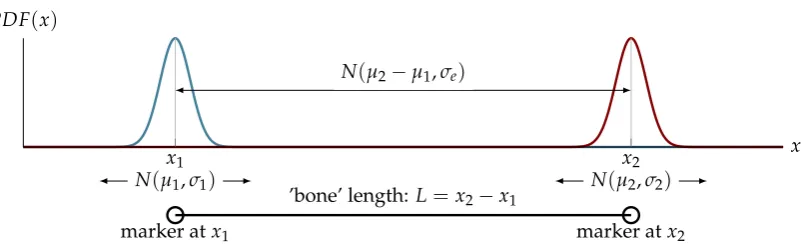
Locating markers in a scene is a continuous process occurring frame-by-frame at the requested sampling frequency. The measurement of the location of a marker can be presumed to be an actual location signal plus additive Gaussian white noise, consequently, locating of each marker location is

an independent statistical process. One dimensional case, as depicted in Fig.1, can be described with

normal probability density function:

loc(Mk)≈xk=N(µk,σk), (1)

where: loc(Mk)denotes actual location of kth marker in a scene. N(·) denotes normal (Gaussian)

92

distribution, which for real location atxk is estimated as a meanµk, and standard deviationσk, that

93

(at best) should be common for all the same markers (of a same size).

94

The typical uncertainty analysis in measurements employs two factors accuracy and precision

95

[18] – the accuracy that describes how close the estimateµkis to actual locationxkand describes the

96

systematic error, whereasσ_kreflects the precision of measurement and describes random part of the

97

error.

98

Extending the estimation of a marker model to the estimation of a length (L) of a bone, it

yields a difference of double marker location measurements, hence its probability density function is described:

length(x1,x2)≈PDF(L) =|N(µ2,σ)−N(µ1,σ)|=N(µe,σe), (2)

where: µe = |x2−x1| - expected (in common sense) mean value,σe - expected standard deviation,

99

which might take different forms, depending on the case:

100

A. σA=σ

√

2 – for two identical (σ1=σ2), independent variances (covarianceσ12 =0),

101

B. σB=

q

σ₁2+σ₁2– for two different (σ16=σ2), independent variances (σ12=0),

102

C. σC=

q

σ₁2+σ₂2−2σ12– for two different (σ16=σ2), correlated variances (σ12 6=0).

103

In this paragraph, we would like to refer in advance to the experimental part described in p.

104

3.1-4. Just to introduce it briefly – the recorded model were two markers of a T-frame template,

105

that was laying steadily on the floor for several hours. T-frame (Fig. 7) is a reference rigid tool for

106

calibrating the OMC systems, where markers are mounted permanently in known locations. The

107

location of two markers and their distance (a bone) were measured with three different types of IR

108

cameras. For the detailed description of the experimental setup please refer to the p.3.

109

The brief results – markers location and their distance are gathered in Tab. 1. It contains

110

estimated parameters for locations and lengths, we provide also theoretically calculated values for

111

length. These are: locations mean values and their standard deviations, covariance, and correlation

(4)

N(µ1,σ1) N(µ2,σ2)

N(µ2−µ1,σe)

marker atx1

’bone’ length:L=x2−x1

marker atx2

x1 x2 x

PDF(x)

Figure 1.Schematic of situation and corresponding theoretic probability - two markers atx1andx2

identifying a single rigid body (bone) of lengthl,

(ρ12) as well, furthermore it contains mean value(µL) and standard deviation (σL) for length as it was

113

reported by the Vicon software. Calculated statistical descriptors are the length (µe) and standard

114

deviation in four variants – σA..C as listed above, with two A variants assuming either markers as

115

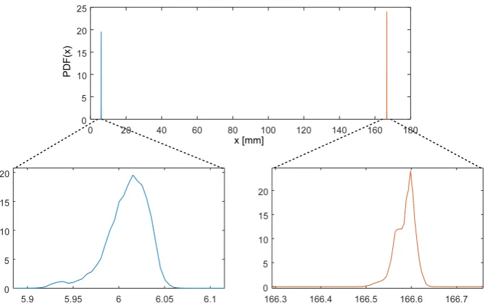
a potential source of variance value. Figure2demonstrates exemplary kernel estimates of location

116

PDFs for one of the camera sets.

117

Table 1.Stats

Measured [mm] Theoretic [mm]

µ1 σ1 µ2 σ2 σ12 ρ12 µL σL µe σA1 σA2 σB σC

T40 166.5863 0.0217 6.0088 0.0234 0.0004 0.8006 160.5818 0.0143 160.5774 0.0307 0.0331 0.0319 0.0143

Bonita 165.9766 0.1635 5.6644 0.1032 0.0011 0.0670 160.3168 0.1870 160.3121 0.2312 0.1459 0.1933 0.1874

Vantage 166.1736 0.0721 5.7363 0.0942 0.0034 0.4980 160.4388 0.0852 160.4374 0.1020 0.1332 0.1186 0.0855

All 166.4613 0.0157 5.9478 0.0176 0.0001 0.4257 160.5176 0.0178 160.5136 0.0222 0.0249 0.0236 0.0179

Generally, the measurement results conform to the theoretic considerations for correlated

118

random variables – obviously the length measurement results confirmed (not included in the paper)

119

in Chi-squared statistical tests their origin in Gaussian distribution with σC. In the considered

120

measurements it is visible in the dispersion of measurements, which is considered as noise. For

121

the low-cost Bonita cameras, the location variance is relatively large, moreover, it is non-correlated

122

to each other (low correlation and covariance), therefore it can be considered as noise. On the other

123

hand, overall dispersion for the high-end T40 cameras is small but highly correlated.

(5)

x [mm]

PDF(

x)

Figure 2.PDF kernel estimation of location forM1andM2using Vicon T40 cameras

159.5 160 160.5 161 161.5

L [mm]

0 5 10 15 20 25 30

PDF(

L)

T40 Bonita Vantage All

Figure 3. Variable PDF estimation of the same length measurement in OMC with different sets of

cameras

The other issue of the error quantification is the lack of reliable ground truth. The Vicon systems

125

return their results with 1/100 mm resolution. It is difficult to obtain a physical template (like the

126

T-frame) manufactured with precision and accuracy comparable or better. For this reason, it is

127

hardly feasible to evaluate the accuracy (bias) of the length estimation with mean values without

128

sophisticated equipment. Fortunately, this aspect is of lesser concern as it describes the systematic

129

error, which is easy to compensate. Moreover, each of the camera sets reports slightly different mean

130

value (see Fig.3), though the discrepancies between the camera sets are on the level rather satisfactory

131

for the most applications – tenth part of a millimeter.

132

The number of cameras used for position reconstruction is another factor, that has a significant influence on the uncertainty of measured position – increasing the number of cameras could be considered as an increasing number of measurements. Multiple measurements of the real value reduce an error of measured value, which is described as a standard error calculated based on the standard deviation for observed value:

σx¯= √σ

(6)

where: N is a number of observations, σ - standard deviation of observed value. This theoretic,

133

quasi-hyperbolic relationship is depicted in Fig. 4. One can denote clearly visible similarity (with

134

some fluctuations) to the real observed decrease in variations for increasing number of cameras

135

shown in Fig.5a.

136

1 2 3 4 5 6 7 8 9 10

.. . 1/√4 1/√3 1/√2 1

N

σx¯

Figure 4.Standard error for estimating actual position with increasing number of measurements

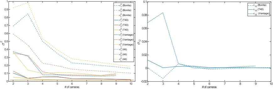
However, as it is depicted in Fig.5b, the covariance is rather constant regardless of the number

137

of cameras (except very low numbers of cameras), whereas the overall variance decreases as the

138

number of cameras grows. It suggests the presence of a process of unknown origin, that is rather

139

common to the markers and affects their registration then physical devices – e.g. it could be either

140

signal processing or a common mechanic micro trembling of cameras. Hence, according to metrology

141

guidelines [18], if the input quantities are correlated in time, then simple experimental mean or

142

standard deviation might be not enough to describe the uncertainty in the system. In such a situation

143

a dedicated tool, namely Allan variance, is recommended.

144

2 3 4 5 6 7 8 9 10 # of cameras

0 0.1 0.2 0.3 0.4 0.5 0.6 0.7 0.8 0.9 1

2

1 2_(Bonita)

2 2_(Bonita)

L 2_(Bonita)

1 2_(T40)

2 2_(T40)

L 2_(T40)

1 2_(Vantage)

2 2_(Vantage)

L 2_(Vantage)

1 2_(All)

2 2_(All)

L 2_(All)

2 3 4 5 6 7 8 9 10

# of cameras -0.02

0 0.02 0.04 0.06 0.08 0.1

12

12(Bonita)

12(T40)

12(Vantage)

Figure 5.Variances (a) and covariances (b) for variable numbers of cameras of different types

2.3. Allan variance 145

Allan variance (AVAR) a two-sample variance and its square root – Allan deviation (ADEV) are

146

statistical descriptors that were developed for the evaluation of the stability of the time and oscillation

147

in clocks. A notable advantage of this approach that there is no need to provide reference value –

148

ground truth.

149

Nowadays, the measure is effectively used for quantifying the noises in the measurement of

150

other quantities [19,20], but particularly for inertial motion capture sensors [21,22].

(7)

Allan variance [8] is defined as:

σy2(τ) =1₂(y(t+τ)−y(t))2, (4)

whereτis the time intersample spacing,h·idenotes expected value.

152

The AVAR analysis consists of identifying the linear parts of certain slopes of the log-log plot of

153

τsteps versus ADEV (square root of AVAR). It is demonstrated in schematic ADEV plot in Fig.6. It is

154

a highly beneficial advantage of the AVAR noise quantification over the power spectral density (PSD)

155

– capability not to clutter different noise processes and to precise discriminate several types at once.

156

However, there is also a disadvantage, AVAR is sensitive to the outliers and requires considering

157

outlier cleaning to obtain reliable results.

158

The conventional types of noise can be identified by their PSD distribution with the power law.

The ’color’ is given as power relation with respect to frequency (S(f) ∝ 1/fα_{). Therefore, overall}

noise characteristics, comprising different basic noise types are:

S(f) =

∑

α

hαfα. (5)

It corresponds to:

σ_y2(τ)≈

∑

τ

hαKατµ, (6)

which for a conventional set of noises yields:

σ_y2(τ)≈Ah−2τ+Bh−1+Ch0τ−1+ (Dh1+Eh2)τ−2. (7)

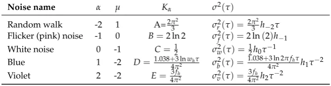
Conventional (color) noise types are gathered in Tab.2,

159

Table 2.Power-law noise types and their Allan variance representation

Noise name α µ Kα σ2(τ)

Random walk -2 1 A=2π2

3 σr2(τ) = 2π

2

3 h−2τ

Flicker (pink) noise -1 0 B=2 ln 2 σ2_f(τ) =2 ln(2)h−1

White noise 0 -1 C= 1₂ σw2(τ) = 1₂h0τ−1

Blue 1 -2 D= 1.038+3 lnwhτ

4π2 σ

2

b(τ) =

1.038+3 ln 2πfhτ 4π2 h1τ

−2

Violet 2 -2 E= 3fh

4π2 σ

2

v(τ) = ₄3fh

π2h2τ

−2

where fhis bandwidth limit for the measurement system.A..Erespective scaling factorsKα.

160

Additionally, two complex distortions can be identified using Allan variance – exponentially

161

correlated (Markovian) and sinusoidal. The Markovian noise is visible in the Allan deviation plot as

162

a single ’bump’ with slopes±1

2. Periodic (sinusoidal) distortion is represented in respective plot as a

163

decaying series of bumps with left-sided slope 1 and right side bump series with constant envelope

164

of a slope−1, however, it is the only case, which is more convenient to be observed and to analyze

165

the distortion in Fourier spectral domain.

166

Correlated noise PSD is given as:

Sc(f) =

(qcTc)2

1+ (2πf Tc)2, (8)

and corresponding Allan variance has a form:

σ_c2(τ) = (qcTc)

2

τ

1− Tc

2τ

3−4e−Tcτ ₊_e−2Tcτ

(8)

where:qcis the noise amplitude,Tcis the correlation time.

167

Sinusoidal noise PSD has a form of two peaks, modeled with Dirac delta:

Ss(f) = 1

2A

2

s(δ(f− f0) +δ(f +f0)), (10)

and respective Allan variance form:

σ_s2(τ) =A2_s sin

2₍

πf0τ)

πf0τ

!

, (11)

where:Asis the amplitude, f0is the frequency,δ(·)is Dirac delta peak.

168

10-3 10-2 10-1 100 101 102 103 104 105

10-6

10-5

10-4

10-3

10-2

-1/2

0

1/2 -1

correlated noise

sinusoidal noise violet/blue noise

white noise

ﬂicker noise

random walk

τ [s]

σy

(

τ

) [mm/s]

Figure 6. Schematic view on Allan Deviation log-log plot (axis values are for illustrative proposes)

3. Materials and Methods 169

3.1. Environment 170

The experimental setup was employed in the Human Motion Laboratory (HML) at the Research

171

and Development Centre of Polish-Japanese Academy of Information Technology in Bytom1. Motion

172

system used in this laboratory consists of a total of 30 Vicon Motion cameras of three different types:

173

• 10 Vicon MX-T40,

174

• 10 Vicon Bonita10,

175

• 10 Vicon Vantage V5.

176

These cameras can record data independently or can be integrated into one larger system with

177

capture volume 9 m x 5 m x 3 m. In order to minimize the impact of external interference like infrared

178

interference from sunlight or vibrations, all windows are permanently darkened and cameras are

179

mounted on scaffolding instead of tripods (as is shown in Fig. 8) The basic information and main

180

differences between used cameras are shown in Table3.

181

(9)

Table 3.Vicon camera difference

Camera model MX-T40 Bonita10 Vantage V5

Resolution [MP] 4 1 5

Max Frame Rate [HZ] 370 @ 4 MP 250 @ 1 MP 420 @ 5 MP

Focal length [mm] 18 4 8.5

Sensor type CMOS CMOSIS CMOS

Type of,LEDs 180 nm NIR 780 nm NIR 850 nm (IR)

Number of LEDs 252 68 22

AOV (HxV) 49.15 x 37.14 70,29 x 70,29 63.5 x 55.1 Dimensions [mm],(HxWxD) 207 x 130 x 75 122 x 80 x 79 166.2 x 125 x 134.1

Weight [kg] 1,8 1 1,6

3.2. Data capture 182

For the noise analysis needs, a special, nine-hour recording of the two 14 mm markers from the

183

calibration T-frame template (wand) was made. The wand (demonstrated in Fig. 7) was placed in

184

the center of motion capture volume. The three other markers were removed. Data was recorded

185

simultaneously by all the 30 cameras at 120 Hz in standard Vicon software (Vicon Blade version

186

3.3.1). The XYZ coordinate system was by default oriented according to the T-frame as it is depicted

187

in Fig.7. Camera calibration was made once with all thirty cameras according to the standard Vicon

188

procedure. The reprojection error for this session, for all the cameras was less than 0.2 pix – mean

189

error for Bonita - 0,1946 pix; Vantage - 0,1891 pix; T40 - 0,1535 pix as reported by the software after

190

the calibration procedure. Additionally, in order to minimize the environmental noise, laboratory

191

technicians were not present in the room during this recording - after the system calibration, all the

192

necessary operations and supervision (start and stop record, system status verification, etc.) were

193

done remotely.

194

Figure 7. Vicon calibration wand schema (T-frame)

3.3. Data processing 195

In the post-processing stage in Vicon Blade (Version 3.3.1) software, markers were reconstructed

196

and labeled only, no other filtering or processing was used. This stage was done several times

197

– separately for each camera configuration (including different numbers of cameras of each type).

198

Reconstruction settings were set to the default, for each camera type except the initial set of 2 cameras

199

of each type, where it required to override the demand of marker visibility by three cameras at least.

200

In this trial, the parameter -’Minimum Cameras to Start Trajectory’had to be set to 2. All those data

201

were used to create the few datasets, containing several realizations of the same sequence:

202

• Data set 1: based on all cameras

203

• Data set 2: based on T40 cameras

(10)

• Data set 3: based on Bonita cameras

205

• Data set 4: based on Vantage cameras

206

The data sets 2-4 consists of 7 trials, in which a different number of cameras used for 3D markers

207

reconstruction (Table4). The location of each camera is shown in the Fig.8. To characterize the noise

208

in different camera type, in all datasets the x,y,z trajectories of both markers and their Euclidean (Eq.

209

12) distance were analyzed.

210

L=d(M1,M2) = p

(x1+x2)2+ (y1+y2)2+ (z1+z2)2 (12)

Table 4.Number and (incrementally) IDs of cameras used for 3D marker reconstruction

Cameras MX-T40 Bonita10 Vantage V5

2 21,26 2,17 3,4

3 +28 +19 +10

4 +22 +16 +11

5 +27 +18 +7

6 +20 +15 +30

8 +24,29 +13,14 +9,8

ALL +23,25 +1,12 +5

Figure 8.Camera locations:a) Schematic view in Vicon Blade software,b) actual setup in HML. Color

denotes camera series: violet – Vantage, green – Bonita, red – T40

Processing operations in Vicon Blade were limited to 3D reconstruction of marker trajectories

211

and exporting the data to the .c3d file format. Further filtering, analysis, and processing of data were

212

done with Matlab (Version R2016b).

213

3.4. Noise parameters estimation 214

For the computing of AVAR from the experimental data we used an implementation by

215

Czerwinski [20]. It implements various AVAR versions, including overlapping estimator, that we

216

chose to use as it is more stable and boundary error prone than conventional one.

(11)

The notable advantage of Allan deviation plots is their simple visual interpretation. Moreover,

218

identification of complex – sinusoidal or correlated – distortions is possible just by visual inspection

219

[21] for the presence of bumps in the plot. Another beneficial feature is the ability to estimate the

220

parameters by simple line or poly-line matching to log-log plot [22]. However, straightforward

221

distinguishing between blue and violet noises is not possible in such a case – to obtain these phase

222

dependant noises it would be necessary to employ much slower variant – modified AVAR estimation.

223

The method for the noise parameters readout from the ADEV curve, used in this research was

224

proposed by Vernotte et al. in [23] – the model employs minimization of weighted least squares

225

(WLS). As it was demonstrated in [19], such an LS model allows even to identify blue and violet

226

noises which are represented jointly byτ−2component.

227

The weighted LS is represented as following minimization problem that reduces the weighted

error between measured AVAR values ˆσ_y2(τ)and a sum of estimated componentsσ_i2(τ)-s :

ˆ

H= arg min

h−2,...,h2,qc,Tc,As,fo≥0



 



∑

τ



  

1 ˆ

σ_y2(τ)



   ˆ

σy2(τ) −

∑

i={v,b,w,_f_,r,c,s}

σ_i2(τ)



   

  

2

  

. (13)

Obtaining reasonable results for such a complexand multideimensional non-linear model is

228

a challenging issue. Therefore, we followed roughly a multi-start hybrid algorithm proposed in

229

[24] – multi-start simulated annealing followed by local minimum search, where multiple starts

230

prevent dependence on the initialization. It follows exploration-exploitation scheme, in the first stage

231

simulated annealing (SA), known for avoiding of getting stuck in local minimum, finds solution close

232

to global optimum, which is then refined by local pattern search – for the latter we propose to use

233

ant colony optimization (ACO), specifically the ACO_R variant for continuous domains [25]. Our

234

additional modification is in the initialization stage of the ACO solver, which is at start populated

235

with values jittered around the solution returned by the SA stage. Exemplary regression results

236

are visually demonstrated in Fig. 9, compared with ordinary (non-weighted) LS obtained with

237

Levenberg-Marquardt algorithm.

238

10-3 10-2 10-1 100 101 102 103 104

[s]

3 4 5 6 7 8 9 10

y

(

) [mm/s]

10-3

allan deviation

LS (Levenberg-Marquardt):135389 WLS (SA+ACO)1:0.0045466 WLS (SA+ACO)2:0.0049994 WLS (SA+ACO)3:0.0048763 WLS (SA+ACO)4:0.0050471 WLS (SA+ACO)5:0.0047075 WLS (SA+ACO)6:0.0049197 WLS (SA+ACO)7:0.004868 WLS (SA+ACO)8:0.0050131 WLS (SA+ACO)9:0.0045466 WLS (SA+ACO)10:0.0046885

Figure 9.Regression results for an excerpt from the experimental data, demonstrates complex ADEV

(12)

As it was mentioned in the p. 2.3 it is necessary to remove the outliers before the AVAR

239

estimation. For that purpose Hampel filter [26] was employed. It checks the signal whether it is

240

larger than the 3 sigma rule threshold computed robustly on the median absolute deviation (MAD)

241

within a sliding window (in our case 1 second of the past and future values) and replaces outlying

242

values with the local median.

243

3.5. Remarks on the results 244

During the data analysis, two issues emerged, its worth to mention them in advance as they

245

could contaminate the results or cause confusion during the interpretation. First, that while recording

246

there occurred a slight seismic crump. The second issue was the failure of one of the cameras (IR LED

247

emitter) during the recording.

248

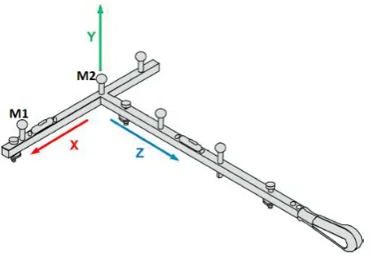
The crump can be observed in the trajectories of the markers (Fig.10a) as a heavy outlier. It has

249

a significant effect on the Allan variance results (see Fig. 10b). That fact draws attention to the need

250

for the careful screening of the measurements for the outliers and proper filtering if necessary – such

251

as the aforementioned Hampel filter.

252

(a)

10-2 10-1 100 101 102 103

10-4

10-3

10-2

10-1

y

All cameras with crump All cameras without crump

(b)

Figure 10. Position X,Y,Z of marker M1 based on data set 1 (a) with crump present, (b) ADEV of

marker distance based on data with and without crump.

The second issue was identified because of the noise levels for data set 4 (Vantage cameras).

253

They were aberrant, for some camera combination the noise levels were increasing when taking more

254

cameras into the reconstruction process. It appeared that one of the cameras was out of order and it

255

would have broken soon after our recordings. Therefore, we excluded it from our analyses and we

256

used up to 9 cameras in the reconstruction for the Vantage data set. Fig. 11illustrates, how such a

(13)

10-2 100 102 104 10-2

10-1

y

x₁

10-2 100 102 104

10-2 10-1

x₂

10-2 100 102 104

10-2 10-1

L

3 9 10

Number of cameras

Figure 11. ADEV for Vantage cameras demonstrating the performance loss due to one damaged

camera (tenth).

failing device, increases the noise in the results forxdimension – the most contributing to the length

258

(L). It is visible in the figure, that we observe larger ADEV values for 10 cameras than for 9, another

259

noteworthy fact is that markers positions are affected to different extents, and the distance is therefore

260

affected to an intermediate extent. The reason for such an observation remains unclear as the internal

261

details of triangulation in Vicon software are kind of a black box. We suspect the inner quality control

262

procedure, that could, for example, select just some subset of cameras.

263

There were also indirect consequences of the failing camera. We could observe slight cross-talk

264

of distortions to the other cameras mounted at similar heights (Vantage and T40), resulting in the

265

presence of short term correlated noise (verified in p4.5). Fortunately-or-not it resulted finally in

266

much more complex ADEV curves we had to analyze, proving that the proposed method is capable

267

to adapt to all the noise types known from the Allan variance literature. The exeplary ADEV curve,

268

obtained for the data after changing the failing camera is included in AppendixBfor comparison. It

269

demonstrates ADEV of the whole system in the facility free of the distortions caused the failing IR

270

LEDs.

271

4. Results and discussion 272

4.1. Overview 273

Using the single long sequence recorded with a regime as described in sections3.1-3.3, we have

274

obtained a pool of sequences obtained with different camera sets. The results were analyzed with an

275

overlapping Allan variance estimator. These results are grouped by camera type and presented as

276

families of Allan deviation plots in Fig.12with a varying number of cameras used in the process.

277

Next, Allan variance noise component parameters were estimated with the procedure described

278

in p. 3.4. The presence and number of correlated and periodic components were examined visually,

279

the verification, whether they are not coming from the periodic distortion, was done by examination

280

of the PSD estimator. The noise parameter estimation results are demonstrated in Figs. 14and15,

281

in logarithmic and linear scales to adapt to large range of values. Numerical values are attached in

282

AppendixAin TablesA1–A3.

283

Finally, the less conventional noises were considered in p.4.5. These are multiple occurrences of

284

correlated noise and periodic distortion.

285

4.2. Overall ADEV characteristics 286

Overall ADEV characteristics for all camera types – T40, Bonita and Vantage are shown in Fig.12.

287

They reveal that theσyvalues gradually decrease with the increasing number of cameras, however,

288

there are some ’drops’ along the camera number axis. That suggest, that certain camera setup is

289

notably better suited for the recorded object – these setups are: 3 cameras for T40, 5 cameras for

290

Bonita, and 4 cameras for Vantage.

291

Another interesting observation in the overall plots can be denoted when analyzing ADEV plots

292

for measured values along the temporal axis. Theσyvalues for the distanceLare larger than for the

(14)

(15)

contributing locationsx1andx2within the range of short-time noisesτ≈ 10−2. . . 101, although for

294

the longer time ranges these values are on par or even ADEV values are smaller for the distance than

295

for contributing locations. Apparently, flicker and random walk noises do not add in the system.

296

We can also observe all the slopes (-1, -1/2, 0, 1/2) from the Tab.2in the characteristics plots. The

297

presence of random walk could be a bit confusing at first, if we omit the results of Jensenius [12], one

298

could expect such distortion not to appear. The triangulation process is done frame-by-frame in the

299

system, therefore the position of a marker should be steady, with flicker, white and higher frequency

300

color noises present. However, there might be implicit denoising present in the system done by low

301

pass filtering, such filters act as integrators, therefore they could introduce some low-frequency noises

302

from the higher noise components.

303

4.3. Comparing the camera types 304

The logical corollary of results demonstrated in the previous paragraph is a direct comparison of

305

camera types. In Fig.13we demonstrate the ADEV plots for each of the camera types at its maximum

306

performance configuration (all cameras). It shows length (L) and marker positions inxas the most

307

important dimension. Comparing the camera types by visual plot inspection confirms the expected

308

outcome, that low-cost Bonita cameras have much higher ADEV values (are more noise affected) than

309

two other camera types. However, ADEV values of up-to-date Vantage cameras indicate that they are

310

more noise affected than relatively old T40s.

311

10-2 10-1 100 101 102 103

10-3 10-2 10-1

x₁ x₂ L

10-2 10-1 100 101 102 103

10-3 10-2 10-1

10-2 10-1 100 101 102 103

10-3 10-2 10-1

T40 (10 cameras) Vantage (9 cameras) Bonita (10 cameras) all (29 cameras)

y

Figure 13. ADEV for maximal numbers of cameras of each type separately and altogether.

4.4. Estimation of basic noise coefficients 312

Several remarks on the noise colors present in the system, that are based on the noise estimated

313

coefficients (Figs.14and15):

314

• Random walk and white noise diminishing with the increasing number of cameras, roughly

315

follow quasi-hyperbolic characteristics described with Eq.3,h≈10−5

316

• Flicker and blue noise levels orders of magnitude are relatively constant with low-moderate

317

valuesh≈10−10

318

• Violet noise levels are negligibly smallh≈10−20..10−300

319

We could also observe intense peak fluctuations in plots ofh coefficient characteristics. They

320

could originate from two potential sources – numerical errors in the optimization process, and/or

321

very specific camera geometric configuration, that could improve or degrade the results. However,

322

the general rule (Eq.3) of decreasing uncertainty with an increasing number of measurements could

323

be observed to some extent for all the noise coefficients (h), but violet one, where it rather seems to be

324

random fluctuations.

325

4.5. Unconventional distortions 326

Regarding the less conventional, correlated noises, a series of interesting observation relates to

327

their presence. In Fig. 16a one can observe, that they are mostly independent of the number of

(16)

2 3 4 5 6 7 8 9 10

No of cameras

10-50

100

h-1

[flicker coef]

2 3 4 5 6 7 8 9 10

No of cameras

10-8

10-6

10-4

h0

[white noise coef]

2 3 4 5 6 7 8 9 10

No of cameras

10-50

100

h1

[blue noise coef]

2 3 4 5 6 7 8 9 10

10-300

10-200

10-100

100

h2

[violet noise coef]

No of cameras

2 3 4 5 6 7 8 9 10

No of cameras

10-40

10-30

10-20

10-10

100

2 3 4 5 6 7 8 9 10

No of cameras

10-5

10-4

10-3

10-2

2 3 4 5 6 7 8 9 10

No of cameras

10-20

10-15

10-10

10-5

2 3 4 5 6 7 8 9 10

10-300

10-200

10-100

100

No of cameras

2 3 4 5 6 7 8 9

No of cameras

10-25

10-20

10-15

10-10

10-5

2 3 4 5 6 7 8 9

No of cameras

10-5

10-4

10-3

10-2

2 3 4 5 6 7 8 9

No of cameras

10-30

10-20

10-10

2 3 4 5 6 7 8 9

No of cameras

10-200

10-150

10-100

10-50

100

2 3 4 5 6 7 8 9 10

No of cameras

10-100

10-50

100

h-2

[random walk coef]

T40

x₁

x₂ y₁

y2

z1

z2

L

2 3 4 5 6 7 8 9 10

No of cameras

10-15

10-10

10-5

Bonita

2 3 4 5 6 7 8 9

No of cameras

10-60

10-40

10-20

100 Vantage

Figure 14. Color noises (h−2..h2) coefficients in logarithmic scale; in columns left to right: T40, Bonita,

(17)

2 3 4 5 6 7 8 9 10 No of cameras

0 0.5 1 1.5 2 2.5 h-1 [flicker coef] 10-9

2 3 4 5 6 7 8 9 10

No of cameras 0 0.5 1 1.5 2 h0

[white noise coef]

10-5

2 3 4 5 6 7 8 9 10

No of cameras 0 1 2 3 4 5 6 h1

[blue noise coef]

10-8

2 3 4 5 6 7 8 9 10

No of cameras 0 0.2 0.4 0.6 0.8 1 1.2 h2

[violet noise coef]

10-11

2 3 4 5 6 7 8 9 10

No of cameras 0

2 4 6

8 10-4

2 3 4 5 6 7 8 9 10

No of cameras 0

1 2 3 4

5 10-3

2 3 4 5 6 7 8 9 10

No of cameras 0

1 2 3

4 10-6

2 3 4 5 6 7 8 9 10

No of cameras 0

0.5 1 1.5 2

2.5 10-10

2 3 4 5 6 7 8 9

No of cameras 0

0.2 0.4 0.6 0.8

1 10-5

2 3 4 5 6 7 8 9

No of cameras 0 1 2 3 4 5

6 10-3

2 3 4 5 6 7 8 9

No of cameras 0

1 2 3

4 10-6

2 3 4 5 6 7 8 9

No of cameras 0

0.5 1 1.5 2

2.5 10-8

2 3 4 5 6 7 8 9 10

No of cameras 0 0.5 1 1.5 2 2.5 h-2

[random walk coef]

10-7 T40

x₁ x₂ y1 y2 z1 z₂ L

2 3 4 5 6 7 8 9 10

No of cameras 0

0.5 1 1.5

2 10-5 Bonita

2 3 4 5 6 7 8 9

No of cameras 0

0.5 1 1.5 2

2.5 10-6 Vantage

Figure 15. Color noises (h−2..h2) coefficients in linear scale; in columns left to right: T40, Bonita,

(18)

cameras –Tcandqcparameters remain relatively constant. Moreover, one could note from Fig.16b,

329

that for correlated noises in the system the longer the time constant the lower amplitude. We could

330

also identify three correlated noise ’classes’ of a different correlation time constants. Their sources

331

remain unknown, however, at least we could speculate about their origins based onTc. Removing

332

the failed camera made the first two of them (see App.B) disappear. Hence our guesses are:

333

• 10−2−100s– due to failed camera, though we considered signal processing based first,

334

• 100−101s– due to failed camera, at first we suspected mechanical based microtrembling of

335

camera support,

336

• 102−103s– environmental based such as changes in room temperature.

337

2

4

no of cameras

6 10-4

10-14

10-12 8

10-10

qc

10-8 10-6 10-2

10-4

10 10-2

100 100

Tc

[s]

102 104

T40 Bonita Vantage x y z

10-14 10-12 10-10 10-8 10-6 10-4 10-2 100

qc

10-3 10-2 10-1 100 101 102 103 104

Tc

[s]

Figure 16. Distribution of correlated noisesqcversusTc.

Finally, the occurrences of periodic noise of f0 ≈ 15Hz frequency had to be checked as it was

338

an unexpected outcome. The verification was done using Welch estimator of PSD (see Fig. 17),

339

and it is present in each of the reconstructions using T40 and Vantage cameras. However, it is

340

usually negligibly small phenomenon, barely observable in most of ADEV plots. Its origin cannot

341

be connected with a recording of any specific camera, but since all the cameras were recording

342

concurrently, it is probably due to some environmental source. Cameras appeared sensitive to a

343

different extent, surprisingly vertical dimensions obtained from the T40 cameras were the most

344

sensitive to this distortion. In case of the Vantage or Bonita cameras it is negligibly small. It requires

345

very large zoom to observe appearance of respective bumps in either PSD or ADEV plots.

346

0 10 20 30 40 50 60

Frequency (Hz) -60

-50 -40 -30 -20 -10 0 10 20 30

PSD (dB/Hz)

T40 Vantage Bonita

Figure 17. Exemplary verification of periodic distortion using PSD forz1reconstructed with maximal

(19)

5. Summary 347

In the article, we demonstrated how to evaluate with Allan variance a compound structure of

348

noise present in the optical Mocap system. The proposed tool was invented for situations when the

349

reliable ground truth is inaccessible. We demonstrated, that it provides outcomes convenient for

350

visual inspection to identify qualitatively noise types actually present in the system or to compare

351

two systems. We have also demonstrated how to employ sophisticated solvers to read the noise

352

parameters from the characteristic ADEV curve, even when it gets quite complicated form.

353

For our facility, we proved that the main contribution to the imprecision comes from the random

354

walk and white noise, whereas flicker noise and blue noise contributions are several orders of

355

magnitude smaller. The influence of violet noise is negligibly small. We have identified also the

356

presence of quite a long term (tens of minutes) correlated noise, probably due to environmental

357

influence. The registration of the noise connected with camera failure was an additional and

358

unforeseen outcome.

359

Future works might include extending the basic approach by analysis of AVAR for bone

360

orientation, though it would require preparing quaternionic AVAR. Other interesting aspects are the

361

variability of AVAR depending on the location in the scene, or how much the results are affected

362

by the presence and activities of staff in the lab. The experiments could be also repeated in different

363

Mocap facilities or laboratories of a different kind, but including Mocap as a feature such as interactive

364

rehabilitation platform Motek CAREN2.

365

Acknowledgments:Grant number goes here - will be provided later.

366

Author Contributions: P.S. conceived the idea, provided the theory, and prepared the analysis tools; M.P

367

conducted the experiments and performed the computations; both authors analyzed and discussed the concepts 368

and results; both authors wrote the paper. 369

Conflicts of Interest:The authors declare no conflict of interest. 370

Abbreviations 371

The following abbreviations are used in this manuscript:

372

ACO: ant colony optimization

373

AVAR: Allan variance

374

ADEV: Allan deviation

375

LS: least squares

376

Mocap: motion capture

377

OMC: optical motion capture

378

RMSE: root mean square error

379

PSD: power spectral density

380

SA: simulated annealing

381

SD: standard deviation

382

WLS: weighted least squares.

383

Appendix A. Estimated noise coefficients 384

Allan variance numerical values for noise component parameters, estimated with the procedure

385

described in p. 3.4. Tables A1-A3 demonstrate results for T40, Bonita, and Vantage cameras

386

respectively.

387

(20)

Table A1.Estimated noise parameters of T40 cameras type for 2..10 devices

a)x1

h−2 h−1 h0 h1 h2 qc1 Tc1 qc2 Tc2 qc3 T3 qc4 Tc4

All 1.55e-10 2.37e-13 9.26e-07 1.35e-13 5.59e-106 5.00e-02 1.00e-02 1.33e-02 2.25e-01 2.04e-03 5.89e+00 3.06e-04 2.00e+03

8 2.99e-09 1.33e-12 1.12e-06 2.91e-09 2.01e-15 5.56e-03 1.62e-01 9.80e-03 3.00e-01 1.92e-03 6.36e+00 2.39e-04 2.00e+03

6 2.82e-09 4.50e-12 1.27e-06 5.42e-09 4.54e-136 4.93e-03 5.48e-01 1.21e-02 2.05e-01 2.13e-03 7.03e+00 3.20e-04 2.00e+03

5 1.03e-08 3.62e-12 2.09e-06 9.57e-09 3.92e-226 5.38e-03 5.63e-01 1.43e-02 2.42e-01 3.02e-03 6.30e+00 3.66e-04 2.00e+03

4 3.96e-09 3.24e-12 2.63e-06 1.39e-08 2.40e-16 1.99e-02 1.99e-01 7.45e-03 6.35e-01 3.12e-03 7.22e+00 6.01e-04 2.00e+03

3 9.57e-09 9.04e-12 3.83e-06 9.82e-09 3.15e-32 2.09e-02 1.95e-01 5.62e-03 5.68e-01 4.60e-03 6.57e+00 6.51e-04 1.41e+03

2 7.65e-08 3.26e-18 5.09e-06 4.60e-09 1.96e-21 9.28e-03 4.54e+00 2.46e-02 1.79e-01 7.63e-10 5.74e+01 5.36e-10 1.55e+03 b)y1

h−2 h−1 h0 h1 h2 qc1 Tc1 qc2 Tc2 qc3 Tc3 As f0

All 4.59e-08 6.11e-22 1.40e-06 3.91e-22 1.47e-157 1.58e-02 1.00e-01 4.72e-03 1.00e+00 6.36e-12 6.21e+02 1.75e-03 5.00e-02

8 4.62e-08 2.45e-20 1.29e-06 1.55e-08 3.73e-172 1.41e-02 1.00e-01 3.78e-03 1.93e+00 6.78e-11 6.73e+02 1.22e-03 2.98e-01

6 4.56e-08 3.32e-19 1.72e-06 2.21e-08 6.14e-265 1.71e-02 1.00e-01 4.26e-03 2.72e+00 4.65e-11 3.65e+02 1.75e-03 2.98e-01

5 5.04e-08 1.59e-19 1.73e-06 2.43e-08 1.50e-69 1.76e-02 1.00e-01 4.62e-03 2.70e+00 5.84e-11 8.47e+02 1.72e-03 2.98e-01

4 5.53e-08 3.88e-19 1.58e-06 2.35e-08 2.12e-70 1.99e-02 1.00e-01 5.84e-03 2.54e+00 8.04e-11 6.60e+02 1.51e-03 2.98e-01

3 6.34e-08 5.93e-19 2.06e-06 2.56e-08 8.38e-187 2.03e-02 1.00e-01 5.74e-03 3.62e+00 9.94e-11 3.88e+02 1.38e-03 2.98e-01

2 7.30e-08 1.29e-14 3.58e-08 7.00e-10 1.29e-51 2.91e-01 1.76e-03 8.38e-03 3.72e+00 2.22e-08 9.20e+02 2.99e-03 5.00e-02 c)z1

h−2 h−1 h0 h1 h2 qc1 Tc1 qc2 Tc2 qc3 Tc3 qc4 Tc4 As f0

All 3.23e-09 4.20e-12 1.26e-06 1.04e-13 3.12e-198 1.87e-02 1.00e-01 6.76e-03 5.10e-01 1.69e-03 7.75e+00 1.70e-04 4.43e+02 3.56e-03 1.44e+01

8 5.04e-09 3.53e-13 1.83e-06 9.68e-09 1.36e-105 3.15e-06 5.29e-02 1.23e-02 3.22e-01 2.29e-03 7.66e+00 2.48e-04 6.75e+02 4.19e-03 1.44e+01

2 1.39e-07 1.44e-15 6.49e-06 6.02e-08 2.54e-114 6.43e-07 8.02e-02 3.32e-02 1.53e-01 1.33e-02 3.87e+00 1.19e-08 5.01e+02 6.25e-03 1.41e+01 d)x2

All 3.87e-09 2.76e-49 1.13e-06 1.48e-49 1.15e-233 1.16e-02 1.20e-01 7.82e-03 3.20e-01 1.84e-03 6.67e+00 1.58e-04 2.00e+03

8 7.28e-09 5.06e-13 1.21e-06 3.81e-09 7.99e-16 8.67e-03 2.00e-01 7.56e-03 3.00e-01 2.11e-03 5.85e+00 2.68e-07 6.23e+02

6 8.11e-09 4.65e-12 1.40e-06 5.46e-09 1.46e-14 1.17e-02 1.95e-01 6.44e-03 3.68e-01 2.34e-03 6.27e+00 8.61e-05 2.00e+03

5 1.28e-08 6.62e-13 1.89e-06 9.90e-09 7.36e-175 1.36e-02 2.00e-01 7.82e-03 4.21e-01 3.06e-03 5.69e+00 2.65e-04 2.00e+03

4 1.06e-08 7.01e-13 2.36e-06 9.55e-09 6.19e-43 2.02e-02 1.94e-01 7.42e-03 5.61e-01 3.27e-03 6.42e+00 4.45e-04 2.00e+03

3 5.84e-14 1.90e-13 4.40e-06 5.61e-09 1.75e-50 2.38e-02 1.79e-01 7.00e-03 6.40e-01 4.99e-03 6.26e+00 7.95e-04 1.59e+03

2 1.17e-07 6.66e-18 6.11e-06 2.10e-17 1.25e-33 2.83e-02 1.85e-01 2.75e-03 8.07e-01 1.12e-02 4.24e+00 1.54e-10 1.25e+03 e)y2

h−2 h−1 h0 h₁ h2 qc1 Tc1 qc2 Tc2 qc3 Tc3 As f0

All 4.60e-08 1.19e-22 1.29e-06 2.56e-23 1.83e-163 1.55e-02 1.00e-01 4.85e-03 1.00e+00 1.78e-12 6.32e+02 1.34e-03 3.69e-02

8 4.87e-08 2.22e-20 9.29e-07 1.79e-08 3.87e-23 1.55e-02 1.00e-01 4.86e-03 1.37e+00 3.11e-13 5.27e+01 3.82e-03 1.37e+01

6 4.97e-08 4.97e-22 1.69e-06 1.10e-08 9.16e-25 1.68e-02 1.00e-01 6.71e-03 1.00e+00 1.71e-12 4.53e+02 2.51e-03 2.68e-02

5 6.18e-08 3.91e-21 1.99e-06 1.49e-08 4.88e-23 1.76e-02 1.00e-01 7.23e-03 1.03e+00 7.33e-11 1.42e+03 3.50e-03 2.35e-02

4 7.04e-08 1.11e-19 1.62e-06 1.40e-08 8.68e-23 2.07e-02 1.00e-01 7.57e-03 1.45e+00 5.02e-11 5.73e+02 3.77e-03 2.40e-02

3 7.77e-08 1.15e-18 1.67e-06 2.28e-08 2.64e-309 2.12e-02 1.00e-01 7.22e-03 3.65e+00 1.15e-10 1.20e+03 3.66e-03 1.41e+01

2 9.83e-08 5.57e-12 8.11e-09 3.93e-09 1.25e-15 2.75e-01 2.30e-03 9.90e-03 2.74e+00 6.15e-07 9.29e+02 6.39e-03 1.95e-02 f)z2

h−2 h−1 h0 h1 h2 qc1 Tc1 qc2 Tc2 qc3 Tc3 qc4 Tc4 As f0

All 6.01e-09 2.51e-19 1.11e-06 1.10e-19 1.56e-25 7.49e-02 1.00e-02 1.56e-02 1.98e-01 2.20e-03 5.61e+00 5.15e-11 4.07e+02 1.08e-03 1.70e-01

8 1.13e-08 1.98e-18 2.22e-06 1.29e-09 2.76e-21 5.57e-08 1.03e-02 1.31e-02 2.67e-01 2.63e-03 6.34e+00 1.09e-10 2.01e+02 1.11e-03 1.81e-01

2 2.14e-07 8.77e-18 9.50e-06 1.65e-08 8.49e-49 3.99e-08 5.36e-02 3.34e-02 1.65e-01 1.52e-02 3.96e+00 6.98e-10 1.16e+02 5.07e-09 3.21e-01 g) distance -L

h−2 h−1 h0 h1 h2 qc1 Tc1 qc2 Tc2 qc3 T3 qc4 Tc4 As f0

All 1.11e-09 3.69e-16 2.13e-06 3.64e-17 1.37e-20 1.63e-02 1.63e-01 1.77e-03 4.95e+00 2.78e-04 2.18e+02 6.50e-10 7.88e+02 1.56e-03 3.14e+00

8 1.28e-09 2.73e-16 2.21e-06 8.55e-09 1.08e-64 1.32e-02 2.20e-01 1.84e-03 5.04e+00 1.30e-08 1.93e+02 3.28e-04 2.20e+02 1.81e-03 1.44e+01

Appendix B. Supplementary measurement Allan deviation 388

For the verification, because of the camera failure, we repeated the testing steady sequence

389

capture after replacing the failing camera. In Fig. A1we demonstrate ’z’ dimension of M1 marker

390

for maximal numbers (10) of each camera type and all the cameras together. We could observe that

391

short term correlated noises disappeared, whereas the bumps representing periodic and long-term

392

correlated noises remain.

393

Bibliography 394

1. Szcz˛esna, A.; Skurowski, P.; Pruszowski, P.; P˛eszor, D.; Paszkuta, M.; Wojciechowski, K. Reference Data 395

(21)

Table A2.Estimated noise parameters of Bonita cameras type for 2..10 devices

a)x1

h−2 h−1 h0 h1 h2 qc1 Tc1 qc2 Tc2 qc3 T3

All 1.51e-07 5.10e-14 1.08e-04 4.69e-07 9.44e-24 2.03e-01 4.23e-02 8.49e-07 4.32e+02 5.23e-03 5.84e+02

8 4.22e-07 6.06e-14 2.57e-04 4.45e-15 7.44e-154 8.85e-02 1.24e-01 1.43e-06 2.88e+02 6.70e-03 3.63e+02

6 6.41e-07 3.29e-13 2.79e-04 1.87e-14 1.63e-16 7.32e-02 1.78e-01 3.56e-04 3.66e+02 8.14e-03 3.66e+02

5 1.73e-06 2.04e-06 4.87e-04 1.92e-14 1.63e-74 4.14e-02 1.11e+00 1.25e-02 3.32e+02 3.48e-06 4.75e+02

4 2.15e-06 1.44e-14 7.99e-04 5.05e-14 1.11e-16 6.25e-02 4.36e-01 1.40e-05 3.46e+02 1.35e-02 3.41e+02

3 8.61e-06 1.74e-04 3.22e-03 4.35e-15 1.68e-70 3.23e-01 1.00e-01 6.61e-06 2.56e+02 3.23e-02 2.84e+02

2 4.81e-06 8.80e-05 2.09e-03 8.38e-19 4.38e-52 2.74e-01 1.00e-01 3.18e-05 2.90e+02 2.59e-02 2.81e+02 b)y1

All 3.05e-07 3.40e-15 5.03e-05 5.84e-08 1.16e-34 6.69e-02 4.23e-02 8.00e-03 1.00e+00 1.89e-03 2.80e+02

8 5.37e-07 1.13e-12 5.22e-05 8.25e-07 3.69e-15 4.38e-01 1.05e-02 1.14e-02 1.27e+00 2.08e-03 2.13e+02

6 5.89e-07 1.64e-14 7.07e-05 3.66e-07 6.40e-15 2.39e-01 1.53e-02 1.43e-02 1.43e+00 3.84e-03 2.13e+02

5 3.05e-07 1.87e-14 1.10e-04 1.24e-13 3.13e-73 7.00e-02 1.00e-02 2.04e-02 1.96e+00 7.53e-03 2.39e+02

4 1.52e-06 2.15e-14 1.15e-04 1.73e-06 4.07e-16 7.00e-01 1.00e-02 2.75e-02 1.75e+00 8.78e-03 2.19e+02

3 1.67e-06 4.26e-12 6.83e-04 2.03e-12 1.82e-15 1.00e+00 1.44e-02 3.97e-02 1.26e+00 2.01e-02 3.82e+02

2 3.83e-06 1.16e-12 1.04e-03 2.15e-13 1.69e-31 1.00e+00 1.89e-02 3.84e-02 1.30e+00 2.08e-02 3.72e+02 c)z1

All 1.58e-07 1.14e-14 8.87e-05 2.07e-14 2.67e-231 1.12e-01 6.35e-02 7.39e-08 2.01e+00 2.59e-05 4.44e+02 4.81e-03 4.44e+02

8 2.24e-07 5.38e-13 1.37e-04 3.07e-07 4.51e-135 1.82e-01 3.85e-02 1.50e-02 1.00e+00 5.96e-03 3.46e+02 2.46e-07 1.39e+03

6 1.79e-07 5.87e-14 7.45e-05 1.30e-13 1.02e-53 9.75e-02 7.88e-02 1.40e-07 4.62e+00 1.01e-03 5.00e+02 4.86e-03 5.00e+02

5 2.14e-07 1.81e-14 8.08e-05 4.81e-14 1.17e-16 1.13e-01 6.13e-02 3.04e-03 1.00e+00 2.75e-07 2.72e+02 5.66e-03 3.04e+02

4 8.68e-07 1.47e-14 1.47e-04 1.39e-13 1.26e-75 1.68e-01 4.97e-02 1.40e-02 1.00e+00 6.90e-06 3.58e+02 8.86e-03 3.41e+02

3 1.11e-06 5.33e-19 4.60e-04 7.17e-18 4.83e-55 1.00e+00 1.74e-02 4.29e-07 3.33e+00 3.79e-06 3.46e+02 1.15e-02 3.42e+02

2 1.63e-06 2.21e-13 8.59e-04 1.76e-13 1.46e-124 1.00e+00 1.91e-02 2.25e-07 3.42e+00 1.18e-06 9.87e+02 1.49e-02 3.08e+02 d)x2

All 2.84e-08 1.72e-15 3.75e-05 4.99e-16 6.55e-278 6.39e-02 9.30e-02 2.06e-07 1.96e+02 3.80e-03 2.89e+02

8 2.60e-08 2.22e-21 6.59e-05 2.49e-17 5.03e-136 8.46e-02 9.43e-02 5.75e-07 1.93e+02 5.32e-03 2.34e+02

6 1.26e-07 2.89e-06 9.24e-05 6.32e-17 7.76e-23 1.01e-01 1.18e-01 5.15e-06 1.86e+02 7.25e-03 1.82e+02

5 2.56e-07 5.80e-16 8.06e-05 3.26e-13 2.45e-10 2.02e-01 4.48e-02 4.89e-08 1.96e+02 3.50e-03 2.22e+02

4 2.28e-07 1.87e-13 1.97e-04 1.48e-15 1.24e-29 1.48e-01 1.07e-01 2.77e-07 1.78e+02 9.28e-03 1.85e+02

3 2.84e-07 3.01e-04 7.19e-04 1.58e-12 2.72e-20 4.52e-01 5.79e-02 3.65e-02 5.95e+01 7.31e-03 9.28e+02

2 1.23e-06 7.34e-04 7.60e-04 3.99e-06 9.54e-48 7.65e-01 2.94e-02 6.96e-02 3.21e+01 1.87e-02 2.63e+02 e)y2

All 2.49e-07 8.04e-16 2.97e-05 1.15e-16 9.63e-203 6.98e-02 9.21e-02 4.87e-03 5.87e+01 6.49e-10 7.55e+02

8 3.58e-07 1.49e-15 4.00e-05 5.21e-17 1.23e-19 6.87e-02 9.73e-02 3.83e-03 5.96e+01 1.26e-09 5.54e+02

6 3.55e-07 3.23e-16 6.27e-05 8.38e-17 1.34e-84 1.01e-01 9.35e-02 7.53e-03 5.43e+01 1.51e-08 6.63e+02

5 6.67e-08 7.32e-35 4.09e-05 4.11e-14 8.14e-56 9.46e-02 5.76e-02 2.30e-07 2.40e+02 2.46e-03 8.78e+02

4 4.91e-07 1.26e-15 9.85e-05 4.51e-17 1.74e-80 1.39e-01 8.15e-02 7.58e-03 6.38e+01 4.36e-09 4.58e+02

3 1.17e-07 2.90e-13 2.36e-04 8.80e-14 2.58e-64 2.10e-01 8.00e-02 1.28e-02 6.35e+01 2.52e-03 1.00e+03

2 2.75e-07 5.17e-05 3.92e-04 4.11e-13 1.22e-16 2.50e-01 7.43e-02 2.18e-02 5.30e+01 3.78e-03 6.58e+02 f)z2

All 1.09e-07 2.60e-16 2.66e-05 5.01e-15 1.27e-17 6.71e-02 7.44e-02 1.92e-08 3.79e+00 2.06e-07 3.26e+02 4.26e-03 2.72e+02

8 7.80e-08 4.66e-16 4.29e-05 2.39e-14 6.73e-17 8.26e-02 6.47e-02 9.21e-08 1.90e+00 5.16e-07 2.99e+02 4.56e-03 3.49e+02

6 9.31e-08 8.69e-32 3.32e-05 8.88e-19 1.54e-41 5.64e-02 8.44e-02 1.41e-07 2.41e+00 3.86e-07 3.71e+02 3.98e-03 3.56e+02

5 1.25e-17 5.20e-14 2.47e-05 3.35e-07 1.92e-15 1.90e-01 2.02e-02 2.22e-07 2.62e+00 6.31e-07 9.16e+02 2.85e-03 1.39e+03

4 2.27e-07 1.22e-27 6.65e-05 7.89e-08 2.24e-16 8.96e-02 6.13e-02 1.72e-08 6.01e+00 4.84e-03 2.41e+02 8.49e-08 1.32e+03

3 3.29e-07 2.29e-14 2.18e-04 1.37e-14 1.90e-17 1.06e-01 1.26e-01 1.84e-07 2.95e+00 1.04e-07 3.77e+01 9.09e-03 1.83e+02

2 5.91e-07 6.08e-12 4.52e-04 5.51e-13 1.14e-80 1.93e-01 9.98e-02 1.97e-02 1.00e+00 6.15e-03 2.67e+02 1.72e-02 1.00e+02 g) distance -L

All 3.66e-07 1.07e-14 1.42e-04 9.68e-07 1.64e-57 2.71e-01 3.80e-02 3.60e-06 5.77e+02 4.54e-03 6.29e+02

8 4.76e-07 1.65e-14 3.66e-04 6.23e-07 7.35e-134 2.54e-01 4.96e-02 6.34e-08 7.52e+02 5.71e-03 5.66e+02

6 8.36e-07 2.17e-14 4.73e-04 4.08e-14 1.44e-281 2.32e-01 7.01e-02 4.49e-07 6.75e+02 7.86e-03 3.67e+02

5 1.67e-06 6.51e-13 1.09e-03 9.42e-14 8.56e-85 1.23e-01 1.65e-01 1.35e-06 4.90e+02 1.09e-02 3.77e+02

4 2.13e-06 7.89e-14 1.29e-03 4.91e-13 7.31e-101 3.31e-01 7.02e-02 9.45e-06 5.40e+02 1.21e-02 5.22e+02

3 1.78e-05 2.76e-04 4.52e-03 2.25e-14 5.49e-79 1.00e+00 4.68e-02 3.76e-02 8.31e+01 2.27e-02 2.00e+02

2 1.10e-05 4.28e-04 4.09e-03 1.84e-13 1.29e-38 1.00e+00 4.81e-02 6.18e-02 2.92e+01 3.17e-02 2.00e+02

In Computer Vision and Graphics; Chmielewski, L.J.; Datta, A.; Kozera, R.; Wojciechowski, K., Eds.; 397

Springer International Publishing: Cham, 2016; Vol. 9972, LNCS, pp. 509–520. 398

2. Szcz˛esna, A.; Skurowski, P.; Lach, E.; Pruszowski, P.; P˛eszor, D.; Paszkuta, M.; Słupik, J.; Lebek, K.; Janiak, 399

M.; Pola ´nski, A.; Wojciechowski, K. Inertial Motion Capture Costume Design Study. Sensors2017, 17, 612. 400

3. Nichols, J.K.; Sena, M.P.; Hu, J.L.; O’Reilly, O.M.; Feeley, B.T.; Lotz, J.C. A Kinect-based movement 401

assessment system: marker position comparison to Vicon. Computer Methods in Biomechanics and 402

Biomedical Engineering2017, 20, 1289–1298. 403

4. Al-Amri, M.; Nicholas, K.; Button, K.; Sparkes, V.; Sheeran, L.; Davies, J.L. Inertial Measurement Units 404