Abstract: In multi-objective optimization problems, the optimization target is to obtain a set of

Article

A Weakly Pareto Compliant Quality Indicator

Emanuele Dilettoso, Santi Agatino Rizzo, Nunzio Salerno

Department of Electrical, Electronics and Computer Engineering, University of Catania, Catania 95125, Italy * Correspondence: [email protected].

Abstract: In multi-objective optimization problems, the optimization target is to obtain a set of non-dominated solutions. Comparing solution sets is crucial in evaluating the performances of different optimization algorithms. The use of performance indicators is common in comparing those sets and, subsequently, optimization algorithms. A good solution set must be close to the Pareto-optimal front, well-distributed, maximally extended and fully filled. Therefore, an effective performance indicator must encompass these features as a whole and must be Pareto dominance compliant. Unfortunately, some of the known indicators often fail to properly reflect the quality of a solution set or cost a lot to compute. This paper demonstrates that the Degree of Approximation (DOA) quality indicator, is a weakly Pareto compliant unary indicator that gives a good estimation of the match between the approximated front and the Pareto-optimal front. Moreover, DOA computation is easy and fast.

Keywords: multiple criteria analysis; algorithms performance; Pareto optimality; quality indicator

1. Introduction

The optimized design of industrial applications is often problematic because of the simultaneous occurrence of many conflicting targets [1-3]. In real-world optimization problems, the decision maker needs to have a wide range of solutions to choose from [4]. Some optimization methods solve a single multi-objective function by aggregating different objective functions [5-7]. The choice of weights is the major weakness to this approach [5]. Other multi-objective optimization algorithms (MOOAs) search for a non-dominated solution set [8-10], i.e. a set of multiple alternative solutions. This set is the Approximation Set in the decision space and the Approximated Pareto Front (APF) in the objective functions space. The main goal of such algorithms is to provide an APF matching the Pareto-optimal one. The problem is to assess how well the approximated front fits the optimal one [11]. The notion of optimization algorithms performance involves evaluating the quality of the solution and the required computational effort [12]. This proves troublesome in the case of multi-objective optimization problems: a good approach would be to use a quality indicator (QI), i.e. a function of the APF that simplifies the quantitative performance comparison of different optimization algorithms. The simplest comparison method would be to check whether one APF is better than another with respect to the Pareto dominance relations [11]. Thus, a QI must be able to account for Pareto dominance to properly compare two different algorithms. This is known as “completeness” with respect to Pareto dominance relations, and is the most desired property of a QI. Moreover, when APFs are incomparable with respect to Pareto dominance relations, more information is needed to compare the APFs provided by different MOOAs. In particular, a good MOOA should [13-15]:

1. minimize the APF distance from the Pareto-optimal front;

2. obtain a good (usually uniform) distribution of the solutions found;

3. maximize the APF extension i.e., for each objective the non-dominated solutions should cover a wide range of values (best case: the global optimum of each objective function must be found);

non–dominated solutions set quality by means of a real number [16]; then it is useful to estimate the effectiveness of a MOOA.

Several known UQIs have no or limited completeness as regards Pareto dominance relations and are unable to take into account all the features listed previously. Few UQIs overcome these limitations despite needing much computational effort.

This paper demonstrates the ≻-completeness of the UQI called Degree of Approximation (DOA) [17]. Moreover it is proved its ability to take into account all the four goals as a whole.

To our knowledge, hypervolume is the only ⊳-complete UQI, and for this reason is considered the best UQI for comparing optimization algorithms. Nevertheless, the relation "⊲" differs from "≺" since the former accounts for the case in which an APF contains some solutions of another one but the probability of this specific event is very low, and it can be considered null when the objective functions’ space belongs to the set of real numbers. Therefore, DOA can be used to evaluate the performance of optimization algorithms instead of the Hypervolume since it is proved that DOA is

≻-complete. Note that the calculation of hypervolume is difficult as the number of objective functions increases, while the calculation of DOA is usually very simple and fast even in the case of many-objective optimization.

The paper is organized as follows. Section 2 recalls the definitions and terminology typically used in multi-objective optimization related to the Pareto dominance concept. Section 3 outlines the characteristics of a quality indicator and presents a review of the most common UQIs. Section 4 describes DOA in detail, while Sections 5 and 6 mathematically demonstrate its ≻≻-completeness

≻-completeness, respectively. Section 7 proves DOA compatibility with respect to the “not better” dominance relation. Finally, Section 8 validates DOA with some examples to highlight its accounting for closeness, distribution, extension and cardinality. Conclusions are drawn in Section 9 and minor details of the proof in Section 6 have been reported in Appendices.

2. Definition and Terminology

2.1. Multi-objective optimization problem

Solving a multi-objective optimization problem means finding the optimal and feasible parameter configurations. A feasible solution (configuration) is called a decision vector (x=x1,x2,...,xm)

and is a point in the decision space (X). An objective vector (y=y1,y2,...,ym), a point in the objective space

(Y), is linked to each decision vector by means of evaluating function f. So, a multi-objective optimization problem, with m decision variables (parameters to be set), n targets (objective functions to be optimized), and c constraints (ℓ equality and c-ℓ are inequality constraints), can be mathematically represented as follows.

Maximize or minimize:

( )

x

(

f

( ) ( )

x f x f

( )

x

)

f

y= = ₁ , ₂ ,..., _n (1)

subject to:

( )

( )

x i c

g

i x g

i i

,..., 2 , 1 0

,..., 2 , 1 0

+ + = ≥

= =

 



(2)

where:

(

)

(

)

( )

x i n f

y

Y y y y y

X x x x x

i i

n m

,..., 2 , 1 ,..., ,

,..., ,

2 1

2 1

= =

∈ =

∈ =

(3)

Without loss of generality, in the following it is assumed that each objective function has to be minimized.

Usually, in real-world multi-objective optimization problems, there is no single parameter configuration that simultaneously optimizes all objective functions, i.e. a point does not exist in the decision space that is a global optimum. Thus, solving a real-world optimization problem means offering the designer a set of alternative optimal solutions in the “Pareto dominance” sense.

Pareto dominance - A decision vector x1 _{dominates another decision vector x}2 _iff:

( ) ( )

_x1 _{f x}2 _{i 1,2,...,n and i: f}

( ) ( )

_x1 _{f x}2

f_i ≤ _i = ∃ _i < _i (4)

This relation is denoted as x1≺_x2_{. When one or more of these relations are not satisfied, x}1_does

not dominate x2_{, this condition is denoted as x}1⊀_x2_{. It is worth noticing that, for a single objective}

function, the standard relation ‘less than’ is generally used to define the corresponding minimization problem, while the symbol ‘≺’ represents a natural extension of ‘<’ in the case of multi-objective functions [18].

Pareto optimality - A decision vector x’ is said to be Pareto-optimal iff: '

: x x

X

x∈ 

∃/ (5)

The set that groups this kind of solutions is known as a Pareto-optimal set, and all the solutions of this set are alternative, no one being dominated by the other solutions.

In addition to dominance, other types of relation between the solutions can be defined:

• strictly dominance: a decision vector x1 _{strictly dominates another decision vector x}2 _{(denoted as x}1 ≺≺x2_{) iff:}

( ) ( )

x f x i n

fi 1 < i 2 =1,2,..., (6)

• weakly dominance: a decision vector x1 _{weakly dominates the decision vector x}2 _{(denoted as x}1≼_x2₎

iff:

( ) ( )

x f x i n

fi 1 ≤ i 2 =1,2,..., (7)

Finally, when x1 _{is better than x}2 _{with respect to a subset of objective functions but x}2 _{is better}

than x1 _{with respect to another subset, the two solutions are said incomparable, denoted as x}1 _{|| x}2 _(or x2 _{|| x}1_):

x1⋠_x2 _{∧ x}2⋠_x1

(

2 1

)

2

1_{||x or x ||x}

x

 (8)

Table 1 resumes the dominance relations. It is worth to note that a relation may imply other relations:

x1≺≺_x2_x1≺_x2_x1≼_x2 ₍₉₎

x1⋠_x2_x1⊀_x2_x1⊀⊀_x2 ₍₁₀₎

By relating the solutions of one APF A to those of another APF B it is possible to extend the dominance relations between two solutions to two APFs. Table 2 shows the relations between two APFs.

Table 1. Dominance relations between two solutions [11].

Symbol Relation Description

x1_{≺≺ x}2 strictly dominance

x1 _{strictly dominates x}2 x

1 _{is better than x}2 _{with respect to each objective function}

x1_{≺ x}2 dominance x1 _{dominates x}2

x1 _{is not worse than x}2 _{with respect to each objective function and x}1 _is

better than x2 _{by at least one objective function}

x1 _{weakly dominates x}2

x1 _{|| x}2 Incomparability

x1 _{and x}2 _{are incomparable} x

1 _{and x}2 _{do not weakly dominate each other}

Table 2. Dominance Relations between two APFs [11].

Symbol Relation Description

A ≺≺ B A strictly dominates B each solution belonging to B is strictly dominated by a solution belonging to A A≺ B A dominates B each solution belonging to B is dominated by a solution belonging to A

A⊲ B A is better than B each solution belonging to B is weakly dominated by a solution belonging to A,and A ≠B

A≼ B A weakly dominates B each solution belonging to B is weakly dominated by a solution belonging to A

A || B A and B are incomparable A and B do not weakly dominate each other

3. Quality Indicator

3.1. Definitions

A quality indicator QI is a function q: S →ℝ, where S is the objective functions space, that assigns a real value to a set of APFs belonging to S related to a multi-objective optimization problem. When the function q has just one argument (i.e. one APF), the quality indicator is called “unary”, when it has two arguments (i.e. two APFs) it is called “binary”, and so on.

The aim of a QI is to compare APFs and so QIs are mainly used to indicate if a multi-objective optimization algorithm works any better than others. Some QIs can also be applied as the acceptance criterion to the selection operator of the stochastic search algorithms [19], but DOA is not devised for such a scope.

3.2 Comparison Methods

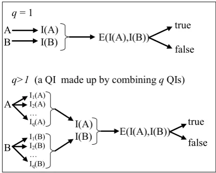
This paper focuses on the use of QIs for evaluating the performances of different optimization algorithms. To do this the QI results must be interpreted by means of an interpretation function E :

ℝq→ _{Bool, where q depends on the size of the QI set. Figure1 shows some examples of interpretation} functions (A and B are two APFs).

Finally, the combination of a quality indicator, I, and an interpretation function, E, is called a comparison method [11], and is referred to as CI,E: CI,E(A,B)=E(I(A),I(B)).

3.3 Compatibility and Completeness

Usually, one or a set of QIs can be useful to compare different optimization algorithms to figure out which works better on a particular class of problems.

Non–dominated solutions are preferred to the dominated ones from the designer’s point of view. Then, when a comparison method shows that APF A is preferable to APF B, A must be better than B. In a similar way, when A is better than B, a comparison method must indicate that A is preferable to B. Such features are known as ⊳-compatibility and ⊳-completeness [11].

Let ► be an arbitrary dominance relation among those defined in Table 2 (≻≻ or ≻ or ⊳). A comparison method CI,E is said ►-compatible if for each possible pair of APFs A and B:

(

AB

)

istrue

CI,E ,

A◄B

(11)

A comparison method CI,E is said ►-complete if for each possible pair of APFs A and B:

A◄B

(

A B

)

istrue CI,E ,

It has been demonstrated [11] that a comparison method based on a UQI (or on a finite combination of UQIs) that is both ⊳-compatible and ⊳-complete cannot exist. Moreover, Pareto dominance is sufficient but not necessary to consider an APF preferable to another: there are pairs of APFs with considerable quality difference which are considered, by Pareto dominance relations, as not comparable [16]. Hence, if a comparison method based on UQI were ⊳-compatible, the indicator could not provide any preference in the case of two incomparable APFs. Therefore, it would be better if the UQI were only compatible with ⋫ [20] and it should take into account all the features (closeness, distribution, extension, cardinality) that are desirable for an APF.

Finally, while a comparison method ⊳-complete is necessary (i.e. when APF A is better than APF B the comparison method must highlight it), when a comparison method shows that A is preferable to B, one of the following two cases must hold:

• A is “better” than B (A ⊲ B);

• A and B are incomparable and A outperforms B with respect to closeness, distribution, extension and cardinality.

q = 1

q>1 (a QI made up by combining q QIs) A

B

I(A)

I(B) E(I(A),I(B))

true

false

A

B

I(A)

I(B) E(I(A),I(B)) true

false

I1(A)

I2(A)

… Iq(A)

I1(B)

I2(B)

… Iq(B)

Figure 1. Comparison method.

3.4 Closeness, distribution, extension and cardinality

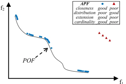
The main target of an optimization algorithm to solve a multi-objective optimization problem is to find an APF as similar as possible to the POF. Hence, as said before, the APF must be:

• close to the POF; Figure 2 represents the extreme cases: an APF exhibiting good closeness only, and an APF with all good features but not close to the POF;

• well distributed (usually uniform); Figure 3 shows an APF exhibiting a uniform distribution only and an APF with all good features but not uniformly distributed;

• very extended (in the best case the global optimum of each objective function belongs to the APF); Figure 4 shows an APF with only a good extension and one with all good features but not extended;

POF

f2

f1

APF ● ▲

closeness poor good distribution good poor extension good poor cardinality good poor

Figure 2. An APF (●) with all good features but not close to the POF and another (▲) that is only close to the POF.

POF

APF ● ▲

closeness good poor distribution poor good extension good poor cardinality good poor f2

f1

Figure 3. An APF (●) with all good features but not uniformly distributed and another (▲) that is only uniformly distributed.

f2

f1

POF

APF ● ▲

closeness good poor distribution good poor extension poor good cardinality good poor

Figure 4. An APF (●) with all good features but not extended and another (▲) that is only extended.

POF f2

f1

f2

f1

APF ● ▲

closeness good poor distribution good poor extension good poor cardinality poor good

Figure 6 shows an APF with all the desired features. A good QI must take into account all these features to give a correct measure of APF quality.

APF

POF

closeness good distribution good extension good cardinality good f2

f1

Figure 6. An APF with all the desired features.

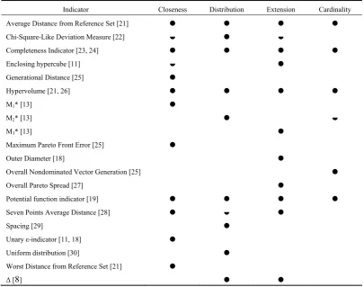
Table 3 points out if a specific feature partially  or totally  affects the value of some UQIs. A heuristic approach has been applied to determine whether a feature (closeness, distribution, extension, cardinality) affects the QI value. In particular, an APF B obtained by improving a given feature of another APF A is expected to have an indicator value better than that of A when the indicator is sensitive to this feature. For example, if an APF is gradually moved towards the POF and the indicator increasingly improves, then the indicator is influenced by the closeness feature. An indicator is “partially” affected by a feature when it sometimes improves and other times it does not change.

The Average Distance from Reference Set indicator [21] (also called Inverted Generational Distance), the Completeness indicator [23,24], the Potential function indicator [19] and the Hypervolume indicator [21, 26] account for all the features but they present some drawbacks.

Table 3. Summary of selected UQIs and features that influence their value.

Indicator Closeness Distribution Extension Cardinality

Average Distance from Reference Set [21]    

Chi-Square-Like Deviation Measure [22]    

Completeness Indicator [23, 24]    

Enclosing hypercube [11]  

Generational Distance [25] 

Hypervolume [21, 26]    

M1* [13] 

M2* [13]  

M3* [13] 

Maximum Pareto Front Error [25] 

Outer Diameter [18]  

Overall Nondominated Vector Generation [25] 

Overall Pareto Spread [27]    

Potential function indicator [19]    

Seven Points Average Distance [28]   

Spacing [29]   

Unary ε-indicator [11, 18] 

Uniform distribution [30]  

Worst Distance from Reference Set [21]  

The Average Distance from Reference Set indicator has the same complexity of DOA, but it is

≻≻-complete only [11].

The Completeness and Potential function indicators are as ≻-complete as the DOA indicator. Nevertheless, the Completeness indicator cannot be directly computed, but can be estimated by drawing samples from the feasible set and computing completeness for these samples. The confidence interval for the true value can be evaluated with any reliability value, given sufficiently large samples [18]. For the Potential function indicator similar considerations hold. Hence, the drawback of both indicators is the high computational cost.

To our knowledge, Hypervolume is the only ⊳-complete UQI, and so is considered the best UQI for comparing optimization algorithms. Nevertheless, the relation A ⊲ B differs from A ≺ B since the former accounts for the case in which B contains some solutions of A but the probability of this specific event is very low, and it can be considered null when the objective functions’ space belongs to the set of real numbers.

Moreover, Hypervolume running time grows exponentially with the number of objective functions [31-34]. The most obvious method for calculating Hypervolume is the inclusion-exclusion algorithm, with complexity O(n2m_{), where n is the number of objectives and m is the number of APF}

points. The fastest methods for calculating Hypervolume (e.g. LebMeasure [35], HSO [36]) lead to a

O(m2_n3_{) complexity. The DOA indicator has a lower computational cost, presenting a O(nMm)}

complexity, where M is the number of POF points.

4. The weakly Pareto compliant quality indicator

The comparison method based on DOA and its associated interpretation function is

≻-complete. While the Hypervolume indicator needs to know the reference point, the DOA calculation needs the knowledge of the POF, like the Average Distance from Reference Set indicator. This is not a drawback in multi-objective algorithm benchmarking which is usually carried out for problems with known POF.

In detail, for an APF A, DOA is computed as follows.

First, given a solution i belonging to the POF, Di,A, is determined from the sub-set of A

containing the solutions dominated by i (Figure 7). Hence, if the number of components belonging to

Di,A is not null (i.e. |Di,A|>0), for each approximated solution a ∈ Di,A the Euclidean distance dfi,a

between a and i is computed as:

[

]



= − =

n

k

i k a k a

i f f

df

1

2 , ,

, (13)

with:

n number of objective functions,

fk,a value of k-th objective function of the approximated solution a, fk,i value of k-th objective function of optimal solution i.

Euclidean distance di,A (Figure 8) between i and the nearest approximated solution belonging to

Di,A is computed in the objective function space as:

( )

   

= ∞

> ∈

=

0 0 min

, , ,

, ,

A i

A i A i a

i A

i

D if

D if D a df

d ₍₁₄₎

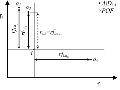
Another quantity ri,A (similarly to di,A) is computed for i considering the solutions of A not dominated by i (i.e. A\Di,A):

( )

   

= ∞

> ∈

=

0 \

0 \ \

min

, , ,

, ,

A i

A i A

i a

i A

i _{if A D}

D A if D A a rf

r ₍₁₅₎

where rfi,a is a ‘reduced’ distance (Figure 9) between i and a non dominated solution a of A (i.e. ∀a ∈

(

)

[

]



=

− =

n

k

i k a k a

i f f

rf

1

2 , ,

, max 0, (16)

Note that, rfi,a is equal to dfi,a when a ∈Di,A. Moreover, defining na (na < n) as the number of functions for which the fk,a-fk,i ≥ 0 (fk,a ≥ fk,i, k=1,..,na and fk,a < fk,i, k= na+1,..,n) expression (16) can be rewritten as:

( )

( )

[

]





= = +

+ −

= a

a n

k

n

n k i a a

i f k f k

rf

1 1

2

, 0 (17)

Finally, defining

si,A = min(di,A,ri,A) (18)

the DOA indicator for the APF A is computed as:



= =

POF

i A i s POF A DOA

1 ,

1 )

( ₍₁₉₎

f2

f1

A POF Di,A

i a1 _a

2

a9

a3

a4 _a 5

a6

a7_a 8

Figure 7. Di,A of a point i belonging to the POF (example with n=2).

f2

f1

Di,A

POF

i

di,A=dfi,a4 a3

a4 _a 5

a6

a7_a 8

a2

a1

f2

rfi,a

1

f1

A\Di,A

POF

i

ri,A=rfi,a₂

rfi,a

2

a9

rfi,a₉

Figure 9. ri,A of a point i belonging to the POF.

Considering two APFs A and B, the proposed quality indicator needs interpreting [11] to affirm either that “A is preferable to B” or “B is preferable to A” or “A and B are equivalent”: the proposed obvious interpretation function is illustrated in Figure 10. Moreover, DOA changes with arbitrary scaling of the objective functions, since the DOA indicator is a distance-based metric, while the relationship between DOA (A) and DOA (B) does not change.

In the following, it is demonstrated that A ≺ B implies “A is preferable to B”, that is DOA (A) < DOA (B), in order to affirm that DOA is a ≻-complete quality indicator.

For the sake of clarity, the ≻≻-completeness of DOA is demonstrated before proving its

≻-completeness.

E(I(A);I(B))

true when DOA(A) < DOA(B)

false otherwise

Figure 10. Interpretation function: pseudo-code to compare A and B by means of DOA(A) and DOA(B).

5. ≻≻-completeness

DOAis a ≻≻-complete quality indicator if DOA(A) <DOA(B) for any pair of APF A and B, with A ≺≺ B.

In the hypothesis that A ≺≺ B, each solution of B is strictly dominated by, at least, one solution of A. To demonstrate that DOA(A) <DOA(B) is sufficient to prove that si,Ais always lesser than si,B

for each point i ∈ POF. In other words, if

si,A< si,B ∀i ∈ POF (20)

then

) ( 1

1 ) (

1 , 1

, _POF s DOA B

s POF A DOA

POF

i B i POF

i A

i < =

=





= =

(21)

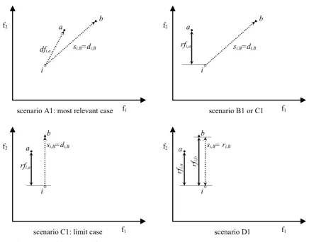
Considering a point i ∈ POF, in the following, b indicates the solution belonging to B which provides si,B and a a solution of A that strictly dominates b (a≺≺b); only four scenarios are possible (see Figure 11):

scenario A1: most relevant case f2

f1

i dfi,a

a b

si,B=di,B

b f2

f1

i a

rfi,a s_i,B=d_i,B

scenario B1 or C1

f2

f1

i a

b si,B=di,B

rfi,a

scenario C1: limit case

f2

f1

i b

si,B= ri,B

rfi,a

scenario D1

rfi,b a

Figure 11. Possible scenarios for A≻≻B.

Note that the other scenarios i≼bΛ i≼a and i || bΛ i≼a are not possible because a≺≺b: in fact, from either i≼bΛa≺≺b and i||bΛa≺≺b follows i⋠a.

Moreover, it is worth to put in evidence the following remarks:

Rmk.1 i ≼a implies that si,A≤dfi,a, in detail: • si,A = dfi,a iff si,A = di,AΛ di,A = dfi,a;

• si,A< dfi,a either if si,A= di,AΛ di,A = dfi,a* < dfi,a (where a*∈A and a*≠ a) or if si,A= ri,A (this implies that ri,A < di,A≤dfi,a).

Rmk.2 i || a implies that si,A≤rfi,a, in detail: • si,A= rfi,a iff si,A= ri,AΛri,A = rfi,a;

• si,A < rfi,a either if si,A = ri,AΛ ri,A = rfi,a* < rfi,a (where a*∈A and a* ≠ a) or if si,A = di,A (this implies that

di,A < ri,A≤rfi,a).

Finally, the inequality si,A < si,B will be proved for the four scenarios A1-D1: this inequality naturally implies the ≻≻-completeness of the DOA indicator.

A1. i ≺≺ b Λ i ≼ a

In this case, i strictly dominates b then si,B = di,B = dfi,b, because b is the solution which provides si,B. Moreover, i ≼a implies that si,A≤dfi,a (see Rmk.1).

So, in order to demonstrate that si,A< si,Bit is sufficient to demonstrate that dfi,a< dfi,b.

Recalling that:

i≼a fk,i≤fk,a, ∀ k=1,..,n

a ≺≺b fk,a < fk,b, ∀ k=1,..,n

[

]

[

]

B i b i a i A i b i n k i k b k n k i k a k a i i k b k i k a k s df df s df f f f f df n k f f f f , , , , , 1 2 , , 1 2 , , , , , ,

, 1,..,

0 = < ≤  = − < − =  = ∀ − < − ≤





= = (22) □

B1. i ≺≺ b Λ i || a

In this case, i strictly dominates b then si,B = di,B = dfi,b, because b is the solution which provides si,B. Moreover, i || a implies that si,A≤rfi,a (see Rmk.2).

So, in order to demonstrate that si,A< si,Bitis sufficient to demonstrate that rfi,a < dfi,b. Proof is

given in the next section because scenario C encompasses scenario B.

C1. i ≺ b Λ i || a

In this case, i dominates b then si,B = di,B = dfi,b, because b is the solution which provides si,B.

Moreover, i || a implies that si,A ≤rfi,a (see Rmk.2).

So, in order to demonstrate that si,A< si,Bis sufficient to demonstrate that rfi,a< dfi,b.

Ordering the n objective functions of solution a in such a way that the first na (with na<n) are

greater than those of i and recalling that:

i || a fk,i < fk,a, ∀ k=1,..,na fk,i≥fk,a, ∀ k=na+1,..,n i ≺b fk,i≤fk,b, ∀ k=1,..,n a ≺≺b fk,a < fk,b, ∀ k=1,..,n

then the following inequalities hold:

[

]

[

]

[

]

B i b i a i A i b i n n k i k b k n k i k b k n k n n k i k a k a i a i k b k a i k b k i k a k s df rf s df f f f f f f rf n n k f f n k f f f f a a a a , , , , , 1 2 , , 1 2 , , 1 1 2 , , , , , , , , , 0 ,.., 1 0 ,.., 1 0 = < ≤  = − + − < + − =  + = ∀ − ≤ = ∀ − < − <









+ = =

= = + ₍₂₃₎

□

D1. i || b Λ i || a

In this case, i and b are incomparable then si,B = ri,B = rfi,b, because b is the solution which provides

si,B. Moreover, i || a implies that si,A≤rfi,a (see Rmk.2).

So, in order to demonstrate that si,A< si,Bit is sufficient to demonstrate that rfi,a< rfi,b.

Ordering the n objective functions of solution a in such a way that the first na are greater than those of i, ordering the n objective functions of solution b in such a way that the first nb are greater than those of i (with na≤nb< n, since a≻≻bΛi || a implies na≤nb, while i || b implies nb < n) and

recalling that:

i || a fk,i < fk,a, ∀ k =1,..,na

fk,i≥fk,b, ∀ k =nb+1,..,n a ≺≺b fk,a < fk,b, ∀ k =1,..,n

then the following inequalities hold:

[

]

[

]

[

]

B i b i a i A i b i n n k n n k i k b k n k i k b k n k n n k n n k i k a k a i b i k b k b a i k b k a i k b k i k a k s rf rf s rf f f f f f f rf n n k f f n n k f f n k f f f f b a b a a b b a , , , , , 1 1 2 , , 1 2 , ,

1 1 1

2 , , , , , , , , , , , 0 0 0 ,.., 1 0 ,.., 1 0 ,.., 1 0 = < ≤  = + − + − < + + − =  + = ∀ − ≥ + = ∀ − < = ∀ − < − <













+ = = + = = = + = + (24) □

6. ≻-completeness

In this section is proved that DOAis a ≻-complete quality indicator. Consider any pair of APF A and B, with A≺B, the ≻-completeness of DOAis demonstrated by proving that si,Ais never greater

than si,B (for each point i ∈ POF) and always exists a point i* ∈ POF for which si*,A is lesser than si*,B:

if

si,A ≤ si,B ∀ i ∈ POF Λ∃ i* ∈ POF : si*,A < si*,B (25) then ) ( 1 1 ) ( 2 , *, 2 ,

*, s s DOA B

POF s s POF A DOA POF i B i B i POF i A i A

i _=

      + <         + =





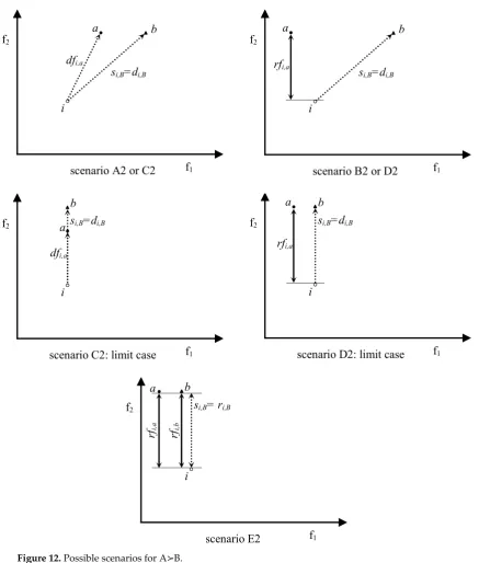
= = (26)

In the following, b indicates the solution belonging to B which provides si,B for a point i ∈ POF and a a solution of A that dominates b (a≺b). Moreover, the ≻-completeness of DOAis proved in the worst and most general case, i.e. when ∀ b∈B ∄a∈A : a≺≺b (i.e. a≺b Λ a⊀⊀b, limit case); only five scenarios are possible (see Figure12):

A2.i≺≺bΛi≺a B2. i≺≺b Λi || a C2.i≺bΛ i ≼ a D2.i≺bΛ i || a E2. i || bΛ i || a

Note that the scenario i || bΛ i≼a is not possible because a≺b: in fact, from i||bΛa≺b

follows i⋠a. Moreover, scenario A2 does not include i=a,differently from section V, because in this case i≺≺b while a≺b Λ a⊀⊀b. Analogously, differently from section V, when i≺b the scenario i ≼

a is possible. Finally, the scenario i ≼ b is not considered becauseA ≺ B, in fact i = b would lead to the absurd a≺b = i.

In order to demonstrate the ≻-completeness of DOA,it is proved that the inequality si,A < si,B is verified ∀i for the three scenarios A2, B2 and C2. While for the remaining two scenarios D2 and E2 we will prove that the following two sufficient conditions hold:

α. si,A ≤si,B

β. ∃i* ∈ POF : si*,A< si*,B.

scenario A2 or C2 f2

f1

i dfi,a

a b

si,B=di,B

b f2

f1

i a

rfi,a

si,B=di,B

scenario B2 or D2

f2

f1

i b si,B=di,B

dfi,a a

scenario C2: limit case

f2

f1

i

a b

si,B=di,B

rfi,a

scenario D2: limit case

f2

f1

i

a b

si,B= ri,B

rfi,a

scenario E2

rfi,b

Figure 12. Possible scenarios for A≻B.

A2. i ≺≺ b Λ i ≺ a

In this case, i strictly dominates b then si,B = di,B = dfi,b, because b is the solution which provides si,B.

Moreover, i ≺a implies that si,A ≤dfi,a (see Rmk.1).

So, in order to demonstrate that si,A < si,B it is sufficient to demonstrate that dfi,a < dfi,b.

Recalling that:

i≺a fk,i≤fk,a, ∀ k=1,..,n

[

]

[

]

[

]

[

]

B i b i a i A i b i n j k k i j b j i k b k n j k k i j a j i k a k a i i k b k i k a k i k b k i k a k s df df s df f f f f f f f f df j k f f f f n k f f f f , , , , , 1 2 , , 2 , , 1 2 , , 2 , , , , , , , , , , , 0 ,.., 1 0 = < ≤  = − + − < − + − =  = − < − ≤ = ∀ − ≤ − ≤





≠ = ≠ = (27) □

B2. i ≺≺b Λ i || a

In this case, i strictly dominates b then si,B = di,B = dfi,b, because b is the solution which provides si,B.

Moreover, i || a implies that si,A ≤rfi,a (see Rmk.2).

So, in order to demonstrate that si,A< si,Bit is sufficient to demonstrate that rfi,a< dfi,b.

Ordering the n objectives f of solution a in such a way that the first na (with na<n) are greater

than those of i and recalling that:

i || a fk,i < fk,a, ∀ k=1,..,na fk,i≥fk,a, ∀ k=na+1,..,n i ≺≺b fk,i < fk,b, ∀ k=1,..,n a ≺b fk,a≤fk,b, ∀ k=1,..,n

then the following inequalities hold:

[

]

[

]

[

]

B i b i a i A i b i n n k i k b k n k i k b k n k n n k i k a k a i a i k b k a i k b k i k a k s df rf s df f f f f f f rf n n k f f n k f f f f a a a a , , , , , 1 2 , , 1 2 , , 1 1 2 , , , , , , , , , 0 ,.., 1 0 ,.., 1 0 = < ≤  = − + − < + − =  + = ∀ − < = ∀ − ≤ − <









+ = =

= = + ₍₂₈₎

□

C2. i ≺ b Λ i ≼ a

In this case, i dominates b then si,B = di,B = dfi,b, because b is the solution which provides si,B. Moreover, i ≼a implies that si,A≤dfi,a (see Rmk.1).

So, in order to demonstrate that si,A< si,Bit is sufficient to demonstrate that dfi,a< dfi,b.

Recalling that:

i≼a fk,i≤fk,a, ∀ k=1,..,n

a ≺b fk,a≤fk,b, ∀ k=1,..,nΛ∃j : fj,a < fj,b

[

]

[

]

[

]

[

]

B i b i a i A i b i n j k k i j b j i k b k n j k k i j a j i k a k a i i k b k i k a k i k b k i k a k s df df s df f f f f f f f f df j k f f f f n k f f f f , , , , , 1 2 , , 2 , , 1 2 , , 2 , , , , , , , , , , , 0 ,.., 1 0 = < ≤  = − + − < − + − =  = ∀ − < − ≤ = ∀ − ≤ − ≤





≠ = ≠ = (29) □

D2. i ≺ b Λ i || a

In this case, i dominates b then si,B = di,B = dfi,b, because b is the solution which provides si,B.

Moreover, i || a implies that si,A≤rfi,a (see Rmk.2).

So, in order to demonstrate that si,A≤si,Bit is sufficient to demonstrate that rfi,a≤dfi,b.

Ordering the n objectives f of solution a in such a way that the first na (with na<n) are greater than those of i and recalling that:

i||a fk,i < fk,a, ∀ k=1,..,na fk,i≥fk,a, ∀ k=na+1,..,n

i ≺b fk,i≤fk,b, ∀ k=1,..,nΛ∃h : fh,i < fh,b a ≺b fk,a≤fk,b, ∀ k=1,..,nΛ∃j : fj,a < fj,b

then the following inequalities hold:

[

]

[

]

[

]

B i b i a i A i b i n n k i k b k n k i k b k n n k n k i k a k a i a i k b k a i k b k i k a k s df rf s df f f f f f f rf n n k f f n k f f f f a a a a , , , , , 1 2 , , 1 2 , , 1 1 2 , , , , , , , , , 0 ,.., 1 0 ,.., 1 0 = ≤ ≤  = − + − ≤ + − =  + = ∀ − ≤ = ∀ − ≤ − <









+ = = + = = ₍₃₀₎ □

Note that rfi,a is strictly lesser than dfi,b when 1 ≤ j ≤na, since:

[

]

_

[

]



= = − < − a a n k i k b k n k i k a

k f f f

f 1 2 , , 1 2 , , (31)

Otherwise si,A≤si,B. In particular, rfi,a = dfi,b iff fk,a = fk,b∀ k=1,..,naΛfk,i = fk,b∀ k= na+1,..,n. In this case,

obviously, fh,i < fh,a = fh,b with 1 ≤ h≤na and fj,a < fj,i = fj,b with j > na. As said before, the proof that∃i* ∈

POF : si*,A< si*,B has been reported in Appendix A. E2. i || b Λ i || a

In this case, i and b are incomparable then si,B = ri,B = rfi,b, because b is the solution which provides si,B. Moreover, i || a implies that si,A ≤rfi,a (see Rmk.2).

Ordering the n objectives f of solution a in such a way that the first na are greater than those of i, ordering the n objectives f of solution b in such a way that the first nb are greater than those of i (with na≤nb< n, since a≺bΛi || a implies na≤nb, while i || b implies nb < n) and recalling that:

i || a fk,i < fk,a, ∀ k=1,..,na fk,i≥fk,a, ∀ k=na+1,..,n

i || b fk,i < fk,b, ∀ k =1,..,nb fk,i≥fk,b, ∀ k =nb+1,..,n

a ≺b fk,a≤fk,b, ∀ k=1,..,nΛ∃j : fj,a < fj,b

then the following inequalities hold:

[

]

[

]

[

]

B i b i a i A i

b i n

n k

n

n k i k b k n

k

i k b k

n

k

n

n k n

n k i k a k a

i

b i

k b k

b a i

k b k

a i

k b k i k a k

s rf rf s

rf f

f f

f

f f rf

n n k f

f

n n k f

f

n k f f f f

b

a b

a a

b b

a

, , , ,

,

1 1

2 , , 1

2 , ,

1 1 1

2 , , ,

, ,

, ,

, , , ,

0 0 0

,.., 1 0

,.., 1 0

,.., 1 0

= ≤ ≤



= + − +

−

≤ + + − =



+ = ∀ −

≥

+ = ∀ −

<

= ∀ − ≤ − <













+

= = +

=

= = + = + (32)

□

It is worth to note that:

rfi,a < rfi,b if nb≠na;

rfi,a≤rfi,b if nb = na.

In the last case, rfi,a = rfi,b iff fk,a = fk,b∀ k=1,..,na. In this case, obviously, fj,a < fj,b≤fj,i whit j > na.

As said before, the proof that∃i* ∈ POF : si*,A< si*,B has been reported in Appendix A. 7. ⋫-compatibility

In this section it is proved that DOA is a ⋫-compatible quality indicator. The following remarks are necessary.

Rmk.3

A solution a’ belonging to A does not influence DOA(A) if, ∀i∈ POF:

• si,A < dfi,a’ when a’ is dominated by i;

• si,A < rfi,a’ when a’ is not dominated by i.

In fact, in this case si,A≠dfi,a’ and si,A≠rfi,a’, by which follows that DOA(A) does not change its value if a’ is moved off from A. These means that an APF B = A\{a’} has the same quality indicator value, i.e. DOA(A) =DOA(B). Using DOA seems B equivalent to A while A, having one more solution, is better than B [11]. Then the proposed method is not a ⊳-complete quality indicator. On the other hand, DOA together with its interpretation function is a ≻-complete comparison method, as it is demonstrated before.

Rmk.4

The relation A ⊲ B is equivalent to assume that B = C ⋃ D, where C ⊊ A, D ⋂ A = Ø and ∀b∈D ∃

a∈A : a ≺b. Note that, when C = Ø then A ≺ B. Hence, the difference between case A ≺ B and A ⊲ B is that in the latter B could contains some solutions of A. Moreover, obviously, only the last case includes B ⊊ A (i.e. D = Ø). For these reasons when A ⊲ B, DOA (A) is never greater than DOA (B).

Rmk.5

The relation A || B involves that DOA (A) can be greater or less than or equal to DOA (B). For two generic APF A and B, the ≻-completeness of DOA, together with Rmks 3-5, imply that if DOA (A) < DOA (B) then A ≺ B or A ⊲ B or A || B, i.e. it is sure that B ⋪ A. Then DOA is a

8. DOA validation

To demonstrate that DOA takes into account all features (closeness, distribution, extension, cardinality) three typical POFs have been considered:

• convex and connected;

• non-convex and connected;

• convex and disconnected.

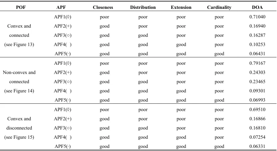
In particular, the DOA unary quality indicator has been computed for different examples of APFs. Both POFs and APFs are drawn in Figure 13-15. Table 4 shows the values of DOA for the APFs considered.

Let's examine the strategy adopted to choose the examples of APF for each POF: the APF B obtained by improving a given feature of APF A is expected to have a better indicator value than that of A if the indicator is sensitive to this feature. For example, if an APF is gradually moved towards the POF and the indicator increasingly improves, then the indicator is influenced by the “closeness” feature. The validation was performed according to these considerations. Hence, from an APF (APF1, indicated in the figures by symbol ) with only poor features, the second APF (APF2, indicated by + ) is created by improving APF1 “closeness” that is by converging APF1 on the POF. Therefore, APF2 has better closeness than APF1 but the same distribution, extension and cardinality. The third APF (APF3, indicated by ○) is obtained by improving the “distribution” of APF2 by uniformly distributing the solutions of APF2. APF3 has better distribution than APF2 but the same closeness, extension and cardinality. The fourth APF (APF4, indicated by □) is created by improving the extension of APF3, preserving the other features. Finally, the fifth APF (APF5, indicated by •) is created by adding new points to APF4, and hence improving the cardinality of APF5 with respect to the fourth APF. It is worth noting that it does not matter in which order the different features are added to the initial APF1, and the order used in Table 4 simply follows the features’ description given in the Introduction.

Whatever the characteristics of the POF, such a strategy highlights that the value of DOA decreases when one feature improves.

The results in Table 4 highlight the ≻-completeness of DOA too. In fact, the first APF is dominated by the others and it has an DOA value worse than those of the other APFs.

Table 4. DOA Evaluation for some typical POF

(symbol in brackets is the marker associated to the APF in figure 13,14,15)

POF APF Closeness Distribution Extension Cardinality DOA

Convex and

connected

(see Figure 13)

APF1() poor poor poor poor 0.71040

APF2(+) good poor poor poor 0.16940

APF3(○) good good poor poor 0.16287

APF4( ) good good good poor 0.10253

APF5(·) good good good good 0.06431

Non-convex and

connected

(see Figure 14)

APF1() poor poor poor poor 0.79167

APF2(+) good poor poor poor 0.24303

APF3(○) good good poor poor 0.23465

APF4( ) good good good poor 0.09301

APF5(·) good good good good 0.06993

Convex and

disconnected

(see Figure 15)

APF1() poor poor poor poor 0.69510

APF2(+) good poor poor poor 0.16866

APF3(○) good good poor poor 0.16810

APF4( ) good good good poor 0.07254

Figure 13. Convex and connected POF (solid line).

Figure 15. Convex and disconnected POF (solid line)..

9. Conclusion

Evaluating the performance of multi-objective optimization algorithms (MOOAs) is very difficult because their comparison involves comparing APFs. QIs are used to measure the goodness of the APF provided by different optimization algorithms to highlight which works better.

Therefore, a QI must be able to account for Pareto dominance to properly compare two different algorithms. Moreover, when APFs are incomparable, further data (closeness, distribution, extension and cardinality) must be taken into account to compare the APFs provided by different MOOAs. Few UQIs are ≻-complete and able to account for the aforementioned features but they need much computational effort.

This paper has described the DOA unary quality indicator that could be very useful in assessing the performance of an MOOA by estimating the match between the approximation front found by the MOOA and the optimal one. It has been proved that it is ≻-complete, ⋫-compatible and requires little computational cost. Moreover, a numerical validation was carried out to demonstrate that it accounts for closeness, distribution, extension and cardinality. An implementation of the DOA indicator is available online: http://wwwelfin.diees.unict.it/esg/DOA.html.

Appendix A

Hypothesis: A ≺ B.

Thesis:

∃i*∈ POF : si*,A = di*,A < si*,B.

Reductio ad absurdum:

In this proof some remarks must be taken into account: I. dfi*,a* = di*,Adfi*,a* ≤dfi*,a’∀a’ ∈ Di*,A

II. dfi*,a* < ri*,Adfi*,a*< rfi*,a’’∀a’’ ∈A\ Di*,A

III. when i ≼ a ≺ b dfi,a < dfi,b (see Section C2)

IV. when i || a ∧ i ≺ b ∧ a ≺ brfi,a≤dfi,b (see Section D2)

V. when i || a ∧ i || b ∧ a ≺ brfi,a≤rfi,b (see Section E2)

VI. ∃i*∈ POF and ∃a*∈A : si*,A = di*,A = dfi*,a*< ri*,A (proved in Appendix B).

Assume the opposite of the thesis:

si*,B≤si*,A (33)

by (33) and Rmks. (VI), follows:

∃ b’∈ Di*,B : si*,B = dfi*,b’ (≤ dfi*,a* = si*,A) (34)

or

∃ b’’∈ B\Di*,B : si*,B = rfi*,b’’ (≤ dfi*,a* = si*,A) (35)

Considering inequality (34), three scenarios are to be analyzed: (a) a* ≺ b’

(b) a’≺ b’, where a’ ∈ Di*,A

(c) a’’≺ b’, where a’’ ∈A\Di*,A

In scenario (a), from Rmk. (III), follows:

A i B i B i b i a i A i A

i d df df s s s

s_*, = _*, = _*,* < _*,'= _*,  _*, > _{*, (36)}

that is in contradiction with (33).

In scenario (b), by considering Rmks. (I) and (III), follows:

A i B i B i b i a i a i A i A

i d df df df s s s

s_*, = _*, = _*,*≤ _*,'< _{*, '}= _*,  _*, > _{*, (37)}

that is in contradiction with (33).

In scenario (c), by considering Rmks. (II) and (IV), follows:

A i B i B i b i a i a i A i A

i d df rf df s s s

s*, = *, = *,*< *, ''≤ *,'= *,  *, > *, (38)

that is in contradiction with (33).

Considering (35), si*,B = rfi*,b’’ implies i* || b’’, i.e. ∄a∈ Di*,A : a≺ b’’. Hence only one scenario

have to be analyzed, in particular a’’≺b’’ , where a’’ ∈A\Di*,A.

By considering Rmks. (II) and (V), follows:

A i B i B i b i a i a i A i A

i d df rf rf s s s

s*, = *, = *,*< *, ''≤ *, ''= *,  *, > *, (39)

that is in contradiction with (33).

Appendix B

Hypothesis: A is a generic APF

Thesis:

∃i∈ POF and ∃a∈A : si,A = di,A = dfi,a< ri,A.

Proof

The proof is given by induction, starting from |A| = 1 and adding to A other solutions recursively. First, only two objective functions (n=2) are considered, then the same procedure is used for the general case (n > 2).

Proof by induction with n=2.

Hypothesis |A| = 1

Proof.

Being A={a} and recalling that POF ≼ A, follows that there exist a solution i∈ POF for which i≼ a, then a∈ Di,A and |A\Di,A| = 0. This implies that:

A i a i A i A i A i a i A i r df d s r df d , , , , , , , < = =  ∞ = ∞ < = (40) □

Hypothesis |A| = 2

Proof.

Being A={a1,a2}, if ∃i∈ POF : i≼a1∧ i≼a2, then a1 and a2 belong to Di,A and |A\Di,A| = 0:

A i a i A i A i A i a i a i a i A i r df d s r df df df d , , , , , 2 , 1 , ,

, min( , )

< = =  ∞ = ∞ < = = (41)

where a is equal to the solution which provides si,A between a1 and a2.

On the other hand, when there not exists such solution i, recalling that POF ≼ A, then exist two solutions i1, i2∈ POF for which i1≼a1 and i2≼a2. Obviously, i1 || a2 and i2 || a1. Hence, without loss of generality it is assumed that:

2 , 2 2 , 2 1 , 2 1 , 2 1 , 1 1 , 1 2 , 1 2 , 1 a i a i a i a i f f f f f f f f ≤ < ≤ ≤ < ≤ (42)

The thesis is proved if si1,A = di1,A = dfi1,a1 < rfi1,a2 = ri1,A∨ si2,A = di2,A = dfi2,a2 < rfi2,a1 = ri2,A. The proof is by reductio ad absurdum. Supposing that:

si1,A=ri1,A=rfi1,a2<dfi1,a1=di1,A∧si2,A=ri2,A=rfi2,a1<dfi2,a2=di2,A (43)

in which:

[

] [

]

[

] [

]

2

2 , 2 2 , 2 2 2 , 1 2 , 1 2 , 2 2 , 1 1 , 1 1 , 2 2 1 , 2 1 , 2 2 1 , 1 1 , 1 1 , 1 1 , 2 2 , 2 2 , 1 i a i a a i i a a i i a i a a i i a a i f f f f df f f rf f f f f df f f rf − + − = − = − + − = − = (44) Note that:

[

] [

]

because the quantities in the brackets are not negative. By (43) and (45) follows: 2 , 2 2 , 2 2 , 1 2 , 1 2 , 1 1 , 1 1 , 2 1 , 2 1 , 1 1 , 1 1 , 2 2 , 2 2 , 2 2 , 2 2 , 1 2 , 1 2 , 2 1 , 2 2 , 1 1 , 1 1 , 2 1 , 2 1 , 1 1 , 1 1 , 1 2 , 1 1 , 2 2 , 2 0 0 i a i a i a i a i a i a i a i a a i a i i a i a i a a i a i i a f f f f f f f f f f f f f f f f df rf f f f f f f df rf f f − + − + + − < − + − + + − <  − + − < < = − − + − < < = − (46) then

[

]

[

]

2 , 2 1 , 2 1 , 1 2 , 1 2 , 2 2 , 2 1 , 2 1 , 2 1 , 2 2 , 2 2 , 1 2 , 1 1 , 1 1 , 1 2 , 1 1 , 1 0 i a i a i a i a i a i a i a i a f f f f f f f f f f f f f f f f − + − = = − + − + + − + + − + − + + − < (47)

that leads to an absurdity because, by (42), it is:

0 0 2 , 2 1 , 2 1 , 1 2 , 1 < − < − i a i a f f f f (48) □

Adding to A other solutions recursively, the previous procedure can be applied to demonstrate that the thesis is always true whatever |A| is.

Proof by induction with n=3.

Hypothesis |A| = 1

Proof. The proof is the same provided for n=2 in (40).

Hypothesis |A| = 2

Proof.

Being A={a1,a2}, if ∃i∈ POF : i≼a1Λ i≼a2, then a1 and a2 belong to Di,A and |A\Di,A| = 0  The proof is the same provided in (41).

On the other hand, when there not exists such solution i, recalling that POF ≼ A then exist two solutions i1, i2∈ POF for which i1≼a1 and i2≼a2. Obviously, i1 || a2 and i2 || a1. Hence, without loss

of generality it is assumed that:

2 , 3 2 , 3 1 , 3 1 , 3 2 , 2 2 , 2 1 , 2 1 , 2 1 , 1 1 , 1 2 , 1 2 , 1 a i a i a i a i a i a i f f f f f f f f f f f f ≤ < ≤ ≤ < ≤ ≤ < ≤ (49)

Likewise for the case of two objective functions the thesis it will be proved that si1,A = di1,A = dfi1,a1

< rfi1,a2 = ri1,A∨ si2,A = di2,A = dfi2,a2 < rfi2,a1 = ri2,A.

The proof is by reductio ad absurdum. Assuming that:

si1,A=ri1,A=rfi1,a2<dfi1,a1=di1,A∧ si2,A=ri2,A=rfi2,a1<dfi2,a2=di2,A

(50)

which imply:

[

] [

]

[

] [

] [

]

[

] [

]

[

] [

] [

]

2