ARBTools: A tricubic spline interpolator for three-dimensional scalar or vector fields.

ARBTools: A tricubic spline interpolator for three-dimensional

scalar or vector fields.

Walker, Paul1,*, Krohn, Ulrich1, Carty, David2

1 Department of Physics, Durham University, South Road, Durham, DH1 3LE, United Kingdom.

2 Department of Chemistry, Durham University, South Road, Durham, DH1 3LE, United Kingdom

* [email protected]

Abstract

ARBTools is a Python library containing a Lekien-Marsden type tricubic spline method for interpolating three-dimensional scalar or vector fields presented as a set of discrete data points on a regular cuboid grid. ARBTools was developed for simulations of magnetic molecular traps, in which the magnitude, gradient and vector components of a magnetic field are required. Numerical integrators for solving particle trajectories are included, but the core interpolator can be used for any scalar or vector field. The only additional system requirements are NumPy.

Keywords

ARBTools, Python, three-dimensional interpolation, spline, vector field, scalar field, smoothing

Introduction

It is often necessary to smoothly interpolate vector or scalar fields known as a set of discrete 2

data points across a grid. For one- and two-dimensional problems cubic and bicubic spline 3

implementations exist (for example, in the SciPy interpolate library [1]), but 4

three-dimensional problems are more difficult. This software was developed for use in 5

modelling the three-dimensional motion of paramagnetic neutral particles through Zeeman 6

decelerators [2] and magnetic traps [3]. These fields are produced by combinations of 7

permanent magnetic and electromagnetic elements with generally no analytic solution. The 8

potentials are calculated, for example using finite element analysis methods, as a series of 9

data points on a grid, which must be interpolated to return the required values for an 10

arbitrary point within the region of interest. 11

The tricubic method described by Lekien and Marsden [4] implements cubic spline 12

interpolation in three dimensions, in an efficient and accurate way. The method was 13

originally motivated by studies of current flow in ocean dynamics [5]; high-frequency radar 14

data give a two-dimensional vector map of the surface of the ocean as a series of discrete 15

points, measured at regular intervals in time. The authors developed their method to 16

smoothly interpolate the time evolution of this velocity field, and note it can equivalently 17

operate on time-independent three-dimensional fields. 18

There are several commonly available implementations of this interpolator in a variety of 19

programming languages, but none were suitable for the specific requirements of our work. 20

ARBTools was written in Python [8], allowing easy modification of the software if needed. 21

Unlike many tools with complex software dependencies the only additional requirement for 22

ARBTools is NumPy [9]. The careful use of NumPy libraries has also allowed the package to 23

be efficient, and in tests it is only moderately slower than an equivalent C implementation. 24

The main difference in ARBTools, however, is the direct availability of the derivatives of an 25

interpolated scalar field, knowledge of these derivatives being a prerequisite for calculating 26

the force arising due to a potential gradient. (Unlike other interpolation methods in which 27

the gradients are recovered via finite-differences, in the tricubic scheme the approximating 28

polynomial function can be analytically differentiated). The software can also directly work 29

with a vector field; for example, in the context of molecular and atomic traps this is needed 30

when calculating the probabilities of non-adiabatic spin transitions [6], or simulating 31

laser-cooling interactions [7]. 32

Interpolation coefficients are calculated on-the-fly and subsequently reused where 33

required to reduce processor time. For arbitrary points inside the interpolation volume the 34

field magnitude, partial derivatives and vector components are readily accessible from a 35

single query. Separate query methods are included for dealing with interpolation of a single 36

point, or for multiple simultaneous coordinates. A fourth-order Runge-Kutta [10] algorithm 37

is implemented for numerically solving particle motion. 38

Although produced for the specific application of modelling low-field-seeking neutral 39

particles, this software has been developed to be more general. It can work directly with 40

either a scalar or vector field input, and is suitable for a variety of applications with any 41

field supplied across a regular, cuboid grid. 42

Implementation and architecture

ARBTools is written in Python [8], with extensive use of NumPy [9]. ‘ARBInterp’ contains 44

the tricubic interpolator and query methods. Any source data presented across a regular 45

grid as either a scalar or vector field can be input into the interpolator, allowing the values 46

of the data to be calculated for arbitrary points within the set. For scalar data the 47

derivatives are directly accessible. Although designed for magnetic fields this software could 48

be used with a wide variety of systems, such as modelling heat flow, or in data processing to 49

smooth contour plots or heatmaps. Example magnetic fields, as both magnitudes and 50

vectors, are available to download along with scripts illustrating the use of the interpolator. 51

These example files also illustrate the expected input format of the data. 52

The ‘ARBTraj’ module contains functions to create a random sample of argon atoms 53

and solve its motion through a quadrupole field. By simply changing mass and magnetic 54

moment values this can be adapted for different atomic species, or a differently shaped 55

magnetic potential could be specified. The included Runge-Kutta integrator can be easily 56

modified to solve particle motion in alternative systems - for example, we have recently 57

discussed simulating the operation of an atomic tweezer apparatus with a colleague. 58

Installation

To install on Linux run ‘sudo python setup.py install’. The interpolator is contained in a file 60

called ‘ARBInterp.py’ and the command ‘from ARBTools.ARBInterp import tricubic’ will 61

import the interpolation class. 62

Usage

To instantiate the class, pass it a source field -e.g. ‘interp = tricubic(sourcefield)’ will 64

create an instance called ‘interp’. Input can be either a scalar field U(x,y,z) as an N x 4 65

(x,y,z,U) array or a vector field B(x,y,z) as an N x 6 (x, y, z, Bx, By, Bz) array. If an N x 4 66

field is passed, the interpolator will automatically default to return the magnitude and 67

gradient of the field. If an N x 6 field is passed it will accept an optional ‘mode’ keyword 68

argument to select one of three modes, (e.g. interp = tricubic(sourcefield, mode=‘kw’)): 69

• Norm: takes the norm of the vector field and return the magnitude and gradient (as 70

three partial derivatives) 71

• Vector: returns the interpolated vector components 72

• Both: takes vector norm, and returns the magnitude and norm of the vector plus the 73

vector components at the interpolation point 74

If no keyword is passed, the interpolator defaults to vector mode. Two query modes are 75

implemented: ‘sQuery’ interpolates a single point within the volume, accepting an input in 76

the form ([x, y, z]). ‘rQuery’ accepts a range of coordinates for simultaneous interpolation, 77

as an array ([x1, y1, z1]...[xn, yn, zn]). For multiple queries rQuery is much more efficient 78

than running sQuery in a loop. 79

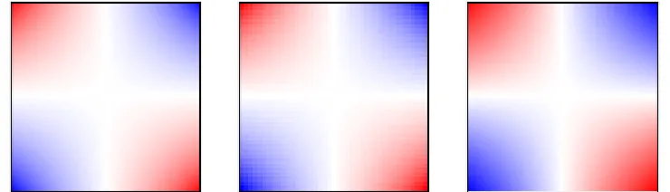
Figure 1. The magnitude of a quadrupole electric field, left, 400 x 400 pixel analytic

solution, centre, 40 x 40 pixel exported subset, right, 400 x 400 pixel interpolation of the subset.

Figure 1 shows an interpolation example. The quadrupole electric field produced by four 80

point charges was calculated as a grid of 4003_{data points; the left plot is a 2D slice through}

81

the central plane. A less dense grid of 403_{points was then calculated, and the middle image}

82

shows a plot through the centre. Lastly, the sparse grid was interpolated to reproduce the 83

4003 _{data, and is shown on the right.}

84

Quality control

ARBTools was written with Python 2.7.12 and NumPy 1.13.3 on Linux Mint 18.3, and has 86

been tested with Python 3.5.2 on the same platform. It has also been tested on Enthought 87

Canopy v2.1.9 on Microsoft Windows 7 and 10. 88

Example input fields and query scripts are available to download from the source 89

repository. Performance benchmarking on 64-bit Linux with an Intel Core i7 CPU shows 90

100 unique interpolations for a given data set take between 20 and 50 ms, depending on 91

which components are being returned. As expected, there is a linear relationship between 92

number of queries and run time. 93

The main constraint when using ARBTools is the amount of memory required to load 94

20 mm on a side with a grid spacing of 0.5 mm contains 413= 68921 grid points, which will 96

load in less than a second with negligible memory usage. The same data sampled at 97

0.25 mm intervals contains 531441 points, this may take several seconds to load and 98

consume≈500 MB memory. At 0.125 mm intervals we have 4173281 points, this may take 99

up to a minute to load and consume over 5 GB of memory. Once loaded, however, querying 100

these different datasets takes almost exactly the same amount of time. 101

The tricubic interpolation method values smoothness of the interpolated function and its 102

first derivatives over absolute accuracy [4]. In order to quantify the errors in this method 103

two types of model were considered; the quadrupole electric field produced by a series of 104

point charges, which can be solved analytically (figure 1), and a magnetic field produced by 105

a permanent magnet, calculated using finite-element analysis with the ‘FEMM’ [11] software 106

package (see figure 2). (Of course, if an analytic solution is available there is no need to 107

interpolate - this is simply a useful calibration tool!) 108

Figure 2. The magnitude of the magnetic field around a ring magnet, left, 400 x 400 pixel

finite-element analysis model, centre, 40 x 40 pixel exported subset, right, 400 x 400 pixel interpolation of the subset.

For both cases a high-resolution source dataset was created, and then a sparse subset of 109

this data was interpolated and compared with it. Figure 3 shows the root-mean-squared 110

errors between the interpolated and ‘true’ values of the calculated fields for a variety of grid 111

intervals. It can be seen that for a given level of accuracy the analytic solution can tolerate a 112

larger grid spacing - this is due to the high gradients at the interface between two materials 113

in finite-element (or boundary volume integral [12]) analysis. In general, consideration of 114

the nature of the data set being interpolated and its structure will inform the grid spacing 115

chosen, which is a compromise between inaccuracy and unwieldiness. These tests were 116

repeated with the interpolator in the ‘EQ Tools’ library; although it does not provide the 117

field derivatives, the magnitudes were found to be the same to within 1×10−6 _%.

118

Figure 3. Root-mean-square error in interpolated data as compared to ‘true’ values from

either a finite-element analysis model or an analytic solution.

(2) Availability

Operating system

ARBTools was developed on Linux Mint 18.3, and has been tested on Windows 7 and 10. 121

Programming language

ARBTools was developed in Python 2.7.12 and has been tested on 3.5.2. Any version of 123

Python from 2.7 upwards should be suitable. 124

Additional system requirements

Several GB of RAM should be suitable for most applications. ARBTools has been used with 126

large datasets on the Durham university supercomputer. 127

Dependencies

Written using NumPy 1.13.3. Earlier versions may work. 129

Software location:

• Name: ARBTools 131

• Persistent identifier: https://doi.org/10.5281/zenodo.2548609 132

• Publisher: Paul A. Walker 133

• Version published: v1.3 134

• Repository: GitHub 135

• Persistent identifier: https://github.com/DurhamDecLab/ARBInterp 136

• Licence: GPL-3.0 137

• Date published: 15/02/2019 138

Language

English 140

(3) Reuse potential

The core of ARBTools is the tricubic interpolator, which can be used with any 142

suitably-formatted input field, for many possible tasks - for example, visualising the shape 143

of a three-dimensional potential or extracting coherent Lagrangian structures from a 144

time-dependent two-dimensional flow. The interpolator has been designed to be imported as 145

a library in Python, and the output from the evaluation methods can easily be passed into 146

third-party code, or output to file for use in non-Python systems. 147

As is, ARBTools can be used to model the trajectories of low-field-seeking argon atoms 148

in a magnetic field. Simply altering the mass and magnetic moment parameters would allow 149

other species to be modelled. If the functions defining the acceleration due to a potential are 150

replaced, trajectories in alternative systems could easily be modelled, for example, the 151

motion of charges in electric fields, or masses moving under gravity. 152

Support may be requested through the project GitHub page: 153

(https://github.com/DurhamDecLab/ARBInterp). The source code is available and may 154

be reused or modified at will subject to the details of the GPL-3.0 licence. 155

Acknowledgements

Many thanks to Dr. Lewis McArd for his invaluable advice on this and other projects. 157

Funding statement

This software was developed as part of research funded by EPSRC grant number 159

EP/N509462/1. 160

Competing interests

“The authors declare that they have no competing interests.” 162

References

1. ‘Interpolation (scipy.interpolate) - SciPy v0.19.0 Reference Guide’, (2017),SciPy.org . 164

Available at: https://docs.scipy.org/doc/scipy/reference/interpolate.html 165

2. McArd, L. M. (2017) ‘A Travelling Wave Zeeman Decelerator For Atoms and 166

Molecules’, PhD thesis, Durham University. 167

3. Walker, P. A. (2019) ‘MT-MOT: a Hybrid Magnetic Trap / Magneto-Optical Trap’, 168

MSci thesis, Durham University. 169

4. Lekien, F. and Marsden, J. (2005) ‘Tricubic interpolation in three dimensions’, 170

International Journal for Numerical Methods in Engineering, Vol. 63, No. 3, pp. 455–471 171

. DOI: 10.1002/nme.1296 172

5. Lekien, F., Coulliette, J. and Marsden, J. (2003) ‘Lagrangian Structures in Very 173

High-Frequency Radar Data and Optimal Pollution Timing’,AIP Conference 174

Proceedings 676, Vol. 162. DOI: 10.1063/1.1612209 175

6. Majorana, E. (1932) ‘Atomi orientati in campo magnetico variabile’,Nuovo Cimento, 176

Vol. 9, pp. 43–50. 177

7. Hanley, R. K., Huillery, P., Keegan, N. C., Bounds, A. D., Boddy, D., Faoro, R., and 178

Jones, M. P. A. (2018) ‘Quantitative simulation of a magneto- optical trap operating 179

near the photon recoil limit’,Journal of Modern Optics, Vol. 65, pp. 667-676, 180

DOI:10.1080/09500340.2017.1401679 181

8. van Rossum, G. (1995) Python tutorial, Technical Report CS-R9526, Centrum voor 182

Wiskunde en Informatica (CWI), Amsterdam 183

9. van der Walt, S., Colbert, S. C., and Varoquaux, G. (2011) ‘The NumPy array: a 184

structure for efficient numerical computation’,Computing in Science and Engineering, 185

Vol. 13, pp. 22-30, DOI:10.1109/MCSE.2011.37 186

10. ‘Runge-Kutta methods’, (2017)Wikipedia . Available at: 187

https://en.wikipedia.org/wiki/Runge-Kutta methods [Accessed April 2017]. 188

11. ‘Finite Element Method Magnetics’ (2019),Meeker, D.. Available at: 189

http://www.femm.info/wiki/HomePage 190

12. Elleaume, P., Chubar, O., Chavanne, J. (1997) ‘Computing 3D Magnetic Field from 191

Insertion Devices’,proc. of the PAC97 Conference, pp. 3509-3511. 192

13. Chilenski, M.A., Faust, I.C. and Walk, J.R. (2017) ‘eqtools: Modular, extensible, 193

open-source, cross-machine Python tools for working with magnetic equilibria’, 194

Computer Physics Communications, Vol. 210, pp. 155-162, 195

DOI:10.1016/j.cpc.2016.09.011. 196