An Approximate Markov Model for the Wright–Fisher Diffusion and Its Application to Time Series Data

| INVESTIGATION

An Approximate Markov Model for the Wright

–

Fisher

Diffusion and Its Application to Time

Series Data

Anna Ferrer-Admetlla,*,†,‡_{Christoph Leuenberger,}§_{Jeffrey D. Jensen,}†,‡_{and Daniel Wegmann*},‡,1

*Department of Biology and§Department of Mathematics, University, of Fribourg, 1700 Fribourg Switzerland,†Department of Life Science, Ecole Polytechnique Federal de Lausanne, 1015 Lausanne, Switzerland, and‡Swiss Institute of Bioinformatics, 1700 Fribourg, Switzerland

ABSTRACTThe joint and accurate inference of selection and demography from genetic data is considered a particularly challenging question in population genetics, since both process may lead to very similar patterns of genetic diversity. However, additional information for disentangling these effects may be obtained by observing changes in allele frequencies over multiple time points. Such data are common in experimental evolution studies, as well as in the comparison of ancient and contemporary samples. Leveraging this information, however, has been computationally challenging, particularly when considering multilocus data sets. To overcome these

issues, we introduce a novel, discrete approximation for diffusion processes, termed mean transition time approximation, which

preserves the long-term behavior of the underlying continuous diffusion process. We then derive this approximation for the particular

case of inferring selection and demography from time series data under the classic Wright–Fisher model and demonstrate that our

approximation is well suited to describe allele trajectories through time, even when only a few states are used. We then develop a Bayesian inference approach to jointly infer the population size and locus-specific selection coefficients with high accuracy and further

extend this model to also infer the rates of sequencing errors and mutations. Wefinally apply our approach to recent experimental data

on the evolution of drug resistance in influenza virus, identifying likely targets of selection andfinding evidence for much larger viral

population sizes than previously reported.

KEYWORDSWright–Fisher model; diffusion approximation; discrete Markov model; hidden Markov model; time-series data

D

in-sights into the evolutionary history of a species and elucidates the interaction between genotype and phenotype, providing important functional information. Unfortunately, a population’s demographic history is a major confounding factor when inferring past selective events, particularly because demographic events can mimic many of the mo-lecular signatures of selection (Andolfatto and Przeworski 2000; Nielsen 2005). Despite efforts to create statistics robust to demography, all currently available methods to detect selection are prone to misinference under nonequi-librium demography.

Some of these issues can potentially be overcome by using multi-time-point data, as the trajectory of even a single allele contains valuable information about the underlying selection coefficient. Owing to advances in sequencing technologies, such multi-time-point data are becoming increasingly

com-mon from experimental evolution (Follet al.2014), from

longitudinal medical or ecological studies (Weiet al.1995; Renzetteet al.2014), and through ancient samples (Sverrisdóttir et al.2014; Wildeet al.2014). However, computationally efficient and accurate methods to infer demography and se-lection jointly from such data sets are still limited.

A natural and common way of modeling such time series data are in a hidden Markov model (HMM) framework, which allows efficient integration over the distribution of unob-served states of the true population frequencies, thus allowing calculation of the likelihood based on the observed samples. Williamson and Slatkin (1999), for instance, developed a maximum-likelihood approach based on such an HMM to infer the population sizeNfrom samples taken at different

Copyright © 2016 by the Genetics Society of America doi: 10.1534/genetics.115.184598

Manuscript received November 7, 2015; accepted for publication March 22, 2016; published Early Online April 1, 2016.

Supplemental material is available online atwww.genetics.org/lookup/suppl/doi:10. 1534/genetics.115.184598/-/DC1.

1_{Corresponding author: Department of Biology, University of Fribourg, Chemin du}

time points. More recently, similar approaches have been de-veloped to infer population size along with the selection co-efficient of a selected locus for which time series data are available (Bollbacket al.2008; Malaspinaset al.2012).

All such approaches, however, are plagued by the problem that the number of hidden frequency states is equal to the population size, which renders HMM applications computa-tionally unfeasible for large populations. Different routes have been taken to overcome this. One approach is to model the underlying Wright–Fisher process as a continuous diffusion process, which is then discretized for numerical integration using a numerical difference scheme (Bollbacket al.2008). Since this approach remains computationally expensive, it was later suggested to directly model the diffusion process on a more coarse-grained grid (Malaspinaset al.2012). Un-der this approach, the generator matrix for the transition between the coarse-grained states is then approximated by

fitting thefirst and second infinitesimal moments. Unfortu-nately, the minimum number of states required is still compu-tationally prohibitive for large values ofg¼2Ns(Malaspinas et al.2012). For this reason, the most recent reported method resorted to simulation-based approximate Bayesian computa-tion (ABC), which allowed the joint inference of locus-specific selection coefficients for many loci (Follet al. 2014, 2015). However, this method requiresfirst estimating the population size under the assumption that all loci are neutral and thus may be biased when many loci are under selection.

Here we introduce a novel framework by approximating the Wright–Fisher (WF) process with a coarse-grained Mar-kov model that exactly preserves the expected waiting times for transition between states. This is achieved by exploiting the theory of Green’s function for diffusion processes. Con-trary to previous approaches, our approximation matches the WF process closely even when only very few states are con-sidered, regardless of g¼2Ns:As we show with extensive simulations and a data application from experimental evolu-tion, our method allows for accurate joint inference of both population size and locus-specific selection coefficients even in the presence of pervasive selection. Further, it is readily extended to incorporate population size changes, sequencing errors, or the appearance of novel mutations.

Models

Mean transition time approximation

LetXðtÞbe a diffusion process on the state space½0;1:This is a continuous-time Markov process with continuous sample paths and with infinitesimal generator

Lf ¼1 2aðxÞ

d2

dx2fþbðxÞ

d

dxf: (1)

For general information about diffusion processes we refer to Durrett (2008, Chap. 7) and Etheridge (2011, Chap. 3).

The classical example in population genetics is the Fisher– Wright diffusion, which we discuss below. We seek tofind a

discrete-state Markov process UðtÞ that approximatesXðtÞ: For this purpose, we subdivide the unit interval½0;1into, not necessarily equidistant, frequencies

u0¼0,u1,. . .,uK21,uK¼1:

These form the states ofUðtÞ:For two statesui;uj;consider the transition time to thefirst visit ofujwhen starting atui:

TuUi/uj ¼infft:UðtÞ ¼uj for Uð0Þ ¼uig:

Similarly we define the transition time for the diffusion pro-cessXðtÞ:We say thatUðtÞis amean transition time approx-imationofXðtÞif

EhTU_ui/uj i

¼EhTX_ui/uj i

(2)

for all pairs of states ui; uj (see Figure 1). This condition guarantees that the paths ofXðtÞandUðtÞexhibit comparable long-term behavior. In the following we show how to con-struct the Markov process UðtÞ from the diffusion process XðtÞ;using the theory of Green’s function.

We begin by recalling some notions for diffusion processes. The natural scale of the processXðtÞis given by

fðxÞ ¼ Z x

cðyÞdy; (3)

wherecðyÞ ¼expð22RyðbðzÞ=aðzÞÞdzÞ;see Durrett (2008, p. 264). The so-called speed measure is defined by

mðyÞ ¼ 1

aðyÞcðyÞ: (4) According to theorem 7.16 in Durrett (2008), Green’s func-tion for an intervalðu;vÞ4½0;1is given by

Gðx;yÞ ¼

2mðyÞðfðvÞ2fðxÞÞðfðyÞ2fðuÞÞ

fðvÞ2fðuÞ ; u#y#x

2mðyÞðfðxÞ2_ff_ððuÞÞðfðvÞ2fðyÞÞ

vÞ2fðuÞ ; x,y#v: 8 > > > < > > > : (5)

Denote by Tx/u orTx/v the time tofirst visit ofuorv, re-spectively, starting at x. Then Tv

u¼minðTx/u;Tx/vÞ is the exit time from the intervalðu1;u2Þ;given the process is atx at timet¼0:One can show (see Durrett 2008, p. 279)

ETv_u¼ Z v

u

Gðx;yÞdy: (6)

Moreover, the probability of exiting at the lower limituis

ℙðTx/v.Tx/uÞ ¼

fðvÞ2fðxÞ

fðvÞ2fðuÞ: (7)

ℙ½UðtþdtÞ ¼ukjUðtÞ ¼uk ¼12qk;kdtþoðdtÞ;

ℙ½UðtþdtÞ ¼ukþ1jUðtÞ ¼uk ¼qk;kþ1dtþoðdtÞ;

and

ℙ½UðtþdtÞ ¼uk21jUðtÞ ¼uk ¼qk;k21dtþoðdtÞ:

The sojourn time of state uk;i.e., the time interval of UðtÞ spent in state uk; is an exponential random variable with parameterqk;k:Since the expectation of this exponential vari-able is 1=qk;k;our condition (2) enforces

qk;k¼

1

ET_kk₂þ1₁ ;

where we write k21 instead of uk; etc., to unburden the notation. From this we get

qk;kþ1¼ℙ

ðTk/kþ1,Tk/k21Þ

ETk_k2þ1₁

and

qk;k21¼ℙ

ðTk/kþ1.Tk/k21Þ

ET_kkþ₂₁1 :

We can now form the tridiagonal generator matrix

Q¼ 0 B B @

0 0 0 0 ⋯

q1;0 2q1;02q1;2 q1;2 0 ⋯ 0 q2;1 2q2;12q2;3 q2;3 ⋯

⋮ ⋮ ⋮ ⋮ ⋮

1 C C A:

The transition matrix of the Markov processUðtÞis given by

PðtÞ ¼exp tQ: (8)

Application to Wright–Fisher models

We consider a classic Wright–Fisher Model of two alleles that segregate in a population of size 2N:Timetis measured in

generations of the Wright–Fisher process. In the presence of a nonvanishing dominance coefficient h the fitnesses of the

three genotypes are given by wAA¼1þs; wAa¼1þhs;

and waa¼1:Under such a model, the infinitesimal mean, which corresponds to the change in allele frequency, is then given by (Ewens 2004, p. 13)

bðxÞ ¼ wAAx

2_þw

Aaxð12xÞ

wAAx2þ2wAaxð12xÞ þwaað12xÞ2 2x

¼xð12xÞsðxþh22hxÞ 1þsxðxþ2h22hxÞ:

(9)

LetXðtÞbe a diffusion process corresponding to the frequency

of allele A. As shown by Lacerda and Seoighe (2014), an

excellent approximation of the Wright–Fisher process is obtained by setting

aðxÞ ¼xð12xÞ

2N (10)

and

bðxÞ ¼skxð12xÞ 1þskx

(11)

in the infinitesimal generator (1), where

sk ¼sð2hþukð122hÞÞ (12)

and

s_k¼sðhþukð122hÞÞ (13)

whenuk21#x#ukþ1:

Note that in the standard diffusion approximation the denominator term in bðxÞ is often omitted. But the above choice yields a much more accurate approximation to the WF process (Lacerda and Seoighe 2014).

From (3) and (4) we get

cðyÞ ¼exp

22

Z y _2Ns k

1þskx

dx

¼ ð1þsyÞ24Nsk=sk (14) Figure 1 Mean transition time approximation of Markov processes. Shown are the realizations of a continuous diffusion processXðtÞ(black) and a discrete-state Markov processuðtÞ(red) starting atuiuntil they reachujfor the first time. If the expected waiting time for such a transi-tion is the same for both processes for all pairs of states

and

fðxÞ ¼ Z x

cðyÞdy¼ 2 1 Mksk

ð1þskyÞ2Mk; (15)

where we have set

Mk¼4N

sk

s_k21: (16)

For the speed measure we obtain

mðyÞ ¼ 1 aðyÞcðyÞ¼

2N

yð12yÞð1þskyÞ

Mkþ1_:

(17)

Consider three consecutive statesuk21;uk;andukþ1:For the probability to exit at the lower state we get

P_Y:¼ℙðTk/kþ1.Tk/k21Þ ¼

fðukþ1Þ2fðukÞ

fðukþ1Þ2fðuk21Þ

¼ ð1þskukÞ2Mk2ð1þskukþ1Þ2Mk ð1þskuk21Þ2Mk2ð1þskukþ1Þ2Mk

¼

1þskukþ1 1þskuk

Mk

21

1þskukþ1 1þskuk21

Mk

21 :

(18)

The probability for exit at the upper state is

P_[:¼ℙðTk/kþ1,Tk/k21Þ ¼12PY:

Observe that Green’s function is calculated by

Gðu_k;yÞ ¼

G_Yðuk;yÞ:¼2P_YmðyÞðfðyÞ2fðuk21ÞÞ; uk21#y#uk

G_[ðu_k;yÞ:¼2P_[mðyÞðfðu_kþ1Þ2fðyÞÞ; u_k,y_#u_kþ1:

Using the quantities calculated above we get for the two parts of Green’s function

GYðuk;yÞ ¼

4NPY

s_kMkyð12yÞ

ð1þs_kyÞMkþ1. . .

 ð1þskuk21Þ2Mk2ð1þskyÞ2Mk

¼4_sNPY

kMk

1þsky

yð12yÞ

1þsky

1þskuk21

Mk

21

! (19)

and

G_[ðuk;yÞ ¼

4NP[

skMkyð12yÞ

ð1þs_kyÞMkþ1. . .

 ð1þs_kyÞ2Mk2ð1þs

kukþ1Þ2Mk

¼4NP[

s_kMk

1þsky

yð12yÞ 12

1þsky

1þskukþ1

Mk! :

(20)

With numerical integration we can determine

ETk_k2þ1₁

¼ EYþ E[¼

Z uk

uk21

GYðuk;yÞdyþ Z ukþ1

uk

G[ðuk;yÞdy:

Specifically, we use the extended Simpson’s rule for the nu-merical integration (Press 2007), which we found to give accurate results with typically only 8 or 10 intervals.

If g¼2Ns is large, we get approximations for Green’s function that allow for analytic expressions of the integrals (seeAppendix). Similarly, analytic expressions can be found in the special cases¼0 (seeAppendix).

Bayesian inference

Consider that at the timesTt;t¼0;. . .;T;samples of sizesMt

were taken from the population and mt allelesAwere

ob-served in these samples. In this section, we describe how the mean transition time approximation introduced above can be embedded into a Bayesian inference scheme to estimate the population size 2Nand the locus-specific selection coefficient jointly from time series data.

As has been noted previously (Williamson and Slatkin 1999; Bollbacket al.2008; Malaspinaset al.2012; Mathieson and McVean 2013; Lacerda and Seoighe 2014; Steinrücken et al.2014), a natural way of modeling both the underlying evolutionary process and the process of sampling is a HMM. Under the assumption that the population size between two time pointsTtandTtþ1is constant atNt;the transition matrix of such an HMM from state UðTtÞ to stateUðTtþ1Þ is calcu-lated by

Pt_¼expðDtQt_Þ;

where Dt¼Ttþ12Tt and the generator matrixQt is

deter-mined as explained above using N¼Nt:We note here that

this framework allows for instantaneous population size changes to occur at every timetduring the HMM. However, we henceforth deal only with situations in which the popu-lation size is assumed to be constant across the whole sam-pling period.

Following previous implementations (e.g., Williamson and Slatkin 1999; Bollbacket al.2008; Malaspinaset al.2012; Mathieson and McVean 2013; Lacerda and Seoighe 2014;

Steinrücken et al. 2014), we assume that the sampling of

alleles from the underlying population frequency is binomial; i.e.,

ℙðmt ¼mjUðTtÞ ¼ukÞ ¼

Mt

m

um_kð12ukÞMt2m:

However, for large sample sizes, the few statesukmay be too coarse grained to capture the region of high emission prob-ability. We thus propose to integrate the emission probabil-ities against a smoothing kernel. We chose to implement a

analytically. Specifically, we chose to use a b-kernel with meanukand standard deviationsk¼ ðukþ12uk21Þ=4;such that the interval½uk₂1;ukþ1corresponds touk62skin the case of equidistant states. Under this choice, the emission probabilities are then calculated by

ℙðmt ¼mjUðTtÞ ¼ukÞ ¼

Mt

m

Bðmþak;Mt2mþbkÞ

Bðak;bkÞ

;

where Bð;Þ is the Beta function and the parametersak

and bk are determined via the moment estimators for a

b-distribution

a_k¼uk

ukð12ukÞ

s2

k 21

; b_k¼akð12ukÞ

uk :

With both transition and emission probability matrices at hand, we calculate the likelihood of the full data, using the standard forward recursion. To be specific, let usfirst define fort¼0;. ..;T theðKþ1Þ3ðMtþ1Þemission probability matrices

Bt

k;m¼ℙðmt¼mjUðTtÞ ¼ukÞ; k¼0;. . .;K;

m¼0;. . .;Mt:

Denotingm1:t ¼ ðm1;. . .;mtÞ;we define the total probability

akðtÞ ¼ℙðm1:t;UðTtÞ ¼ukÞ:

This total probability can be determined efficiently with the forward recursion (Murphy 2012, p. 609)

a_kðtÞ ¼X

K

i¼0

 a_iðt21ÞP_kt2_;i1Bt_i;mt (21)

andakð0Þ ¼B0k;m0:Then one has

ℙðm1:TjuÞ ¼ XK

k¼0

 akðTÞ; (22)

where we made explicit the dependence of this probability on the parameters

u¼ ðs;h;N0;. . .;NT21Þ:

If we impose priors pðuÞ on the parameters, then we can simulate the posterior probabilitypðujm1:TÞwith the usual MCMC scheme using (22) and the Hastings ratio

hu;u9¼min ℙ

m1:Tju9

pu9 ℙðm1:TjuÞpðuÞ  

qu9/u qu/u9;1

! :

Extension of basic model

Sequencing errors: Generally, sequencing errors are

over-come with sufficient coverage. However, in many

appli-cations of next-generation sequencing to experimental evolution, the goal of the sequencing is not to infer indi-vidual genotypes, but instead allele frequencies directly. Under such a setting, each sequencing read is assumed to be from a different individual. In such cases, sequencing errors may lead to false inference, especially when allele frequencies are very small.

probability thatmðiÞt ;theith allele surveyed at timet, isAin the presence of sequencing errors as

ℙmðtiÞ¼AjUðTtÞ ¼uk

¼ ð12eÞukþeð12ukÞ:

Mutational input: We allow for the production of mutant alleles only when the process is in stateu0¼0 oruK¼1:The production of new alleles proceeds at a rate of 2Nmdt:Once a new allele is produced, say when the system is in stateu0; it must get from state 1=2Ninto stateu1:This happens with probabilityP_[¼ℙðT1₌2N/u1,T1=2N/0Þ;which is calculated

according to (7). This yields the transition rate

q0;1¼2Nm ℙ

T1=2N/u1,T1=2N/0

:

Since u1 is close to 0, we can assume that s2sh and

M2N;see (16). Using (7) and (15) we obtain

q0;1¼2Nm

fð0Þ2fð1=2NÞ

fð0Þ2fðu1Þ

¼2Nm12ð1þs=2NÞ

2M

12ð1þsu1Þ2M

2Nm 12ð1þsh=NÞ

22N

12ð1þ2shu1Þ22N

2Nm 12expð22shÞ 12expð24Nshu1Þ:

For the production of a new allele in stateuK¼1 an analogous

argument yields the approximations ss; M4Nð12hÞ

and by (18)

qK;K21¼2Nm ℙ

Tð2N21Þ=2N/1.Tð2N21Þ=2N/uK21

¼

1þsð2N21Þ=2N2M2ð1þsÞ2M ð1þsuK21Þ2M2ð1þsÞ2M

2Nm exp

2sð12hÞ21 exp4Nsð12hÞð12uK21Þ

21:

In the selection-free case,i.e., in the limits/0;the transition probabilities simplify to

q0;1¼

m

u1;

qK;K21¼

m

12uK21:

Implementation

We have implemented the proposed model and the Bayesian inference scheme in an easy-to-use C++ program available on our laboratory website (http://www.unifr.ch/biology/ research/wegmann). While we use standard implementa-tions for most aspects, we note the matrix exponentiation in Equation 8, which is a numerically very demanding problem. A classic algorithm for matrix exponentiation is by diagonalization of the matrix (Moler and Van Loan

1978). While computationally efficient, this algorithm

may be numerically unstable for matrices with large condition numbers, which are typically observed wheng¼2Nsbecomes

large. This was previously observed by Malaspinas et al.

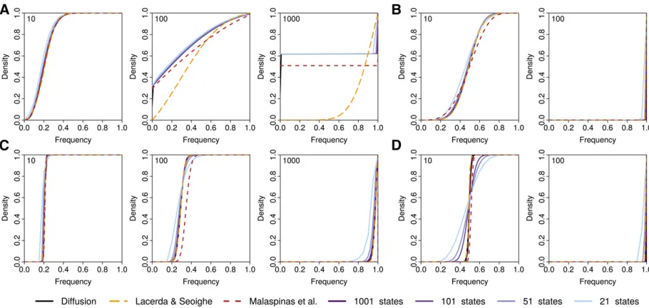
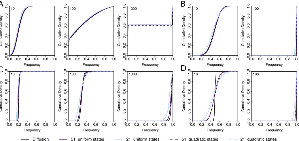
(2012), who addressed this issue using multiple-precision Figure 3 Comparison of different approximations. Shown are the cumulative probability density distributions (CDF) of allele frequencies after 10, 100, and 1000 generations (shown in each top left corner) of selection and random drift starting from a frequency of 0.2 and obtained under the Wright–

Fisher diffusion (black) and three approximations of it: the approximations introduced by Lacerda and Seoighe (2014) (orange) and Malaspinaset al.

arithmetics. Unfortunately, such arithmetics are computation-ally very demanding, leading to slow performance of their implementation.

Here, we propose to alleviate this problem, using the approximation

exp Q

Iþ 1 2nQ

2n ;

which can be calculated by successive quadration. Such matrix multiplications are generally demanding, but can be imple-mented in a computationally efficient manner for generator matrices that are tridiagonal, as each quadration step adds only two additional diagonals and such band matrices can be multiplied efficiently (see Dahlquist and Björk 2008, Chap. 7.4).

We further mention the choice of frequency bins. Malaspinas et al.(2012) report that for their approach, a tighter spacing of frequencies toward the boundaries led to more accurate re-sults, in particular with what they call a“quadratic grid.”We thus chose to implement, apart from a uniformly spaced grid, also a quadratic grid withu0¼0 and

uk ¼uk21þx*ð12xÞ; x¼k2 1 2;

scaled such thatuK ¼1:The major difference of this choice from the quadratic grid proposed by Malaspinaset al.(2012) is that we do not forceu1¼1=2NanduK21¼121=2N;as this would force us to change the frequency bins as a function

of N during the MCMC and hence to recalculate emission

probabilities.

Application to influenza data

Influenza data: We analyzed allele frequency data from

whole-genome data sets of influenza H1N1 obtained in a

recent evolutionary experiment (Renzetteet al.2014). While we refer the reader to the original study for a detailed de-scription of the experimental setup, we summarize the key

point briefly here: Influenza A/Brisbane/59/2007 (H1N1) was

serially amplified on Madin–Darby canine kidney (MDCK)

cells for 12 passages of 72 hr each to prevent any freeze– thaw cycles. After the three initial cycles, samples were passed either in the absence of drug or in the presence of increasing concentrations of oseltamivir, a neuraminidase inhibitor, for another nine passages. At the end of each passage, samples were collected for whole-genome high-throughput population sequencing up to a median cover-age of.50,0003.

For our analysis here we considered only the time points taken during drug treatment (passages 4–12), but considered all 13,395 sites for which data were available (Foll et al. 2014). For each site, wefirst identified the two alleles having the highest frequencies over all passages and considered the minor allele to be the one with the lower frequency at the beginning of the experiment (passage 0). To avoid any bias, all other alleles were treated collectively as the major allele. We estimatedNalong with locus-specific selec-tion coefficientss, the sequencing error ratee, and the per site mutation ratem. We assumed log-uniform priors onN,e, and

m such that log10ðNÞu½1;5; log10ðeÞ ¼u½24;20:3; and log10ðmÞ ¼u½27;21 and a normal prior on the selection coefficients such thats N ð0;0:05Þ:Since viruses are haploid, wefixed the dominance coefficient ath¼0:5:We then ran an MCMC using 51 states for 25,000 iterations during which

each parameter was updated in turn. The first 2000 such

iterations were discarded as burn-in phase.

Simulations:To assess the accuracy of our approximation, we simulated trajectories under the discrete Wright–Fisher pro-cess and the diffusion propro-cess, as well as under the mean transition time approximation and the approximation

pro-posed by Malaspinas et al. (2012). All simulations under

transitions according to the transition matrices calculated under the specific approximations.

To evaluate the power of our method to infer population sizes and selection coefficients, we also simulated data for 20 or 100 unlinked loci withN= 100, 1000, or 10,000. For each of these settings, we set either 20% or 80% of the loci to be under selection, with an equal representation of four selec-tion coefficients:20.1, 20.01, 0.01, and 0.1. All loci, both selected and neutral, had the starting allele frequency set at random. The change in allele frequency from one time point to the next was calculated under the Wright–Fisher model, matching the experimental setup of our application. Specifi -cally, we simulated a total of 117 generations and took a sample of 1000 sequences every 13 generations, unless oth-erwise stated.

Data availability

The authors state that all data necessary for confirming the conclusions presented in the article are represented fully within the article.

Results and Discussion

Mean transition time approximation

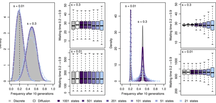
Comparisons of the long-term behavior of the here-introduced mean transition time approximation of the Wright–Fisher process with its discrete realization demonstrate the power of our approximation. In Figure 2 we show the frequency distribution of alleles with an initial frequency of 0.2 after 10 generations of selection and random drift under the dis-crete Wright–Fisher process for different population sizes and different selection strength. As expected from our assump-tions, the distributions obtained under our approximation have identical means and show only a slightly increased var-iance for large selection coefficients and a small number of

states. Thisfinding is further strengthened when comparing this distribution over larger timescales up to 1000 genera-tions (Figure 3), which also illustrates that our approxima-tion leads to accurate loss/fixation ratios. In the situations studied here, all loci correctlyfix in the case of strong selec-tion or whenNis large. In the case ofN¼100 ands¼0:01; however, we estimate that 62.00% or 61.99% of all loci will be lost when using 1001 or 21 states, respectively. This is very similar to the proportion of 62.02% obtained among 33105 simulations with the diffusion approximated here.

A more direct illustration of our assumption is the com-parison of the distribution of waiting times for a specific transition. As shown in Figure 2, our approximation indeed captures the mean transition time perfectly, while again exhibiting an increased variance for large selection coeffi -cients and small number of states. Based on these results, and to keep the computational effort minimal, we use 51 states for all our inference shown below.

Choice of grid

Comparison with related methods

Recently, Lacerda and Seoighe (2014) proposed to approxi-mate the probability distribution of allele frequencies aftert generations by a Gaussian distribution, the mean and vari-ance of which can be obtained iteratively using the delta method. Their approach can easily be applied to the diffusion process studied here (seeAppendix). As shown in Figure 3, the approximation obtained via the delta method and our approximation are very similar over a large range of the pa-rameter space and also agree well with the diffusion process they both approximate. However, due to the assumption of a Gaussian distribution, the approximation obtained with the delta method is less accurate than our approach in describing allele frequencies close to boundaries. This is particularly true when selection is weak enough such that the probability offixation is , 1:0;which results in a bimodal distribution (Figure 3A).

A major advantage of the delta approach, however, is its computational speed, which does not depend on the popula-tion size or the selecpopula-tion strength. Our method is generally much more demanding due to its reliance on matrix calcula-tions rather than simple recursions. But the benefit of our approach lies in the discretization of allele frequencies, with-out which any inference from time-series data is computa-tionally impossible wheneverNis large.

In this regard, our method is closer to that introduced by Malaspinaset al.(2012) that also uses a grid of discretized allele frequencies. In contrast to our method, however, their approach approximates the mean and variance of the infi -nitesimal transition probabilities, rather than those of the resulting waiting times. While Malaspinaset al. (2012) de-rive their approximation for the classic diffusion, it is straight-forward to generalize their approach and apply it to the diffusion studied here (see Appendix). As shown in Figure 3, their approximation holds generally well for most of the range tested, but allele frequencies appear to rise slightly too fast. More importantly, the approximation introduced by Malaspinas et al.(2012) requires substantially more states than our approximation due to the mathematical nature of the approximation. For the case ofN¼10;000 ands¼0:3 shown in Figure 3D, for instance, a minimum of 5813 states are required. In contrast, our approximation is computation-ally stable even with just a handful of states and thus allows us to balance accuracy and computation effort regardless ofN

ors. This difference between the two approaches easily trans-lates into a reduction in computation time of several orders of magnitude when attempting to infer parameters using an HMM and essentially rendering such an analysis unfeasible for large

g¼2Ns with the approximation introduced by Malaspinas

et al.(2012), as has been reported recently (Follet al.2015).

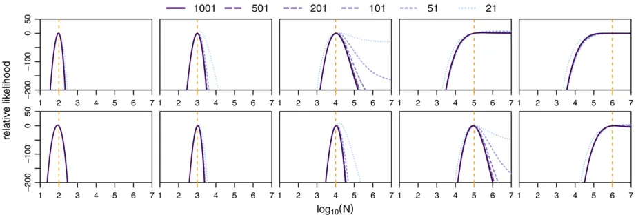
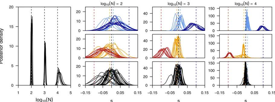
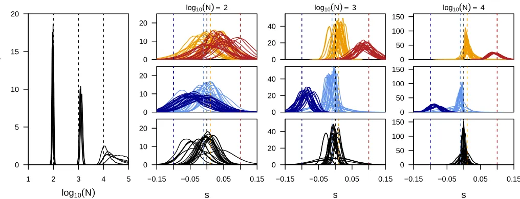
Power to infer population sizes

While allele trajectories are affected by both selection and drift, we aim here to disentangle these effects by integrating information from multiple loci. Wefirst assessed the power to infer population sizes N accurately under ideal conditions, that is, for 100 unlinked loci in the absence of selection. In Figure 4 we show the likelihood surfaces forNobtained with a different number of states, for data simulated under differ-ent population sizes. While this analysis suggests high power to infer small population sizes accurately, it highlights the general issue of inferring large population sizes from changes in allele frequencies, accentuated when fewer states are used. The issue arises from the fact that in large populations and over the short time course of evolutionary experiments in general, the changes in allele frequencies between time points are so small that they are compatible with almost ar-bitrarily large populations. While using fewer frequency states further decreases the resolution of detectable allele frequency changes, we note that this issue is more general and expected to affect all methods for inferring population sizes from such data, particularly when a small number of samples is used. The best way to overcome it is to observe changes in allele frequencies over larger intervals. Indeed, when taking samples every 130 generations instead of every

13, population sizes up to N = 100,000 can be estimated

accurately (Figure 4, bottom row).

Power to infer selection

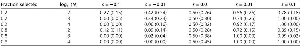
To assess the power of our framework to infer locus-specific selection coefficients, we simulated 100 unlinked loci, of which 20% experienced selection at various strengths. As shown in Figure 5, both the population size and the strength of selection affect the power of this inference. For medium to large population sizes, our method infers even small selection coefficients with high accuracy. When the population size is small, however, inference of selection proves more difficult (Figure 5). While this is generally expected due to the much larger effect of drift in small populations (Ns¼10 for the Table 1 Power to identify loci under selection

Fraction selected log10ðNÞ s=20.1 s=20.01 s= 0.0 s= 0.01 s= 0.1

0.2 2 0.27 (0.15) 0.42 (0.24) 0.50 (0.26) 0.56 (0.26) 0.78 (0.18)

0.2 3 0.00 (0.05) 0.24 (0.24) 0.50 (0.30) 0.74 (0.26) 1.00 (0.00)

0.2 4 0.00 (0.00) 0.06 (0.16) 0.50 (0.32) 0.92 (0.17) 1.00 (0.00)

0.8 2 0.12 (0.11) 0.09 (0.14) 0.50 (0.28) 0.72 (0.15) 0.89 (0.15)

0.8 3 0.00 (0.00) 0.02 (0.04) 0.50 (0.38) 1.00 (0.00) 0.99 (0.02)

0.8 4 0.00 (0.00) 0.00 (0.00) 0.50 (0.45) 1.00 (0.00) 1.00 (0.00)

strongly selected alleles), it is accentuated here by our choice to simulate initial frequencies at random. Indeed, when given ideal starting frequencies (0.1 for positively and 0.9 for nega-tively selected alleles), our method identifies strongly selected alleles accurately even in small populations (Figure S2).

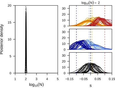
Remarkably, we found the power to infer population sizes as well as locus-specific selection coefficients not to be neg-atively affected under pervasive selection. This is illustrated by comparing the posterior distributions obtained from simula-tions where 80% of all loci were targeted by selection (Figure S3) to those shown here where only 20% were affected by selection (Figure 5). More direct evidence is given in Table 1, where we report the posterior probability fors.0:0 for dif-ferent combinations of population sizes and selection coeffi -cients and actuallyfind higher power to identify selected loci in the case of pervasive selection than when only 20% of all loci were simulated under selection.

For computational efficiency, all results shown here were obtained using 51 states. However, we note a trade-off be-tween power of inference and computational costs. As shown inFigure S4, using very few states (21) may lead to slightly broader posteriors and a small bias toward weaker values of s. Both effects are already largely overcome when using 51 states for most loci, but small improvements are still detect-able with more states (Figure S4).

Application to influenza data

We next applied our approach to publicly available sequencing data of influenza H1N1 segment 6, obtained at multiple time

points throughout an evolutionary experiment in which the virus was exposed to an antiviral drug (oseltamivir) (Renzetteet al.2014). While allele frequencies are gener-ally estimated with high accuracy due to the very high

cov-erage in this experiment (50,0003), sequencing error

may contribute substantially to the observed low-frequency variants. In addition, many of the observed mutations likely entered the population only during the experiment, but their exact time of origin is blurred by both the sequencing error and sampling. We thus extended our framework to estimate the mutation rate as well as the overall sequencing error rate jointly with the demographic and selection parameters.

We applied our extended method to each of the eight segments of the influenza genome individually, but obtained highly concordant results among all segments. As shown in Figure 6, we infer the effective population size during the

experiment to be 7000, a mutation rate of1025_{;and a}

sequencing error rate of1023:8_{:While our estimates of the} mutation and error rates are consistent with published

mu-tation rates for influenza (Nobusawa and Sato 2006) and

RNA viruses in general (Drake et al. 1998) and also with

the employed qualityfilters on sequencing reads (Follet al. 2014), our estimate of the population size is substantially larger than previous estimates of 225 (Foll et al. 2014). While we found our approach to slightly overestimate larger population sizes under the spacing of time points relevant here, there are several arguments supporting a larger popu-lation size. First, the original estimates were obtained under Figure 6 Evolution of drug resistance in influenza. Here we show the posterior distributions on the population size [log10ðNÞ], sequencing error rate (e), mutation rate (m), and locus-specific selection coefficientsslestimated independently for each of the six segments of the influenza genome. For the

the assumption of neutrality at all loci, while our approach infersNjointly with selection. Second, the previous estimates were obtained from a small subset of the data, namely the 147 loci with an observed allele frequency #1% after down-sampling to 1000 reads per locus at no less than three time points. In contrast, our inference is based on the raw data at the complete set of 13,395 loci, including those with small frequencies particularly informative about drift. Third, the original inference accounted for neither sequencing errors nor mutations. In summary, our results argue for a much larger effective population size than previously reported.

Our results on selection, on the other hand, are highly concordant with previous estimates. In Figure 6 we report the posterior distributions on the locus-specific selection coeffi -cients for all polymorphic sites for each of the eight segments of the influenza genome. As expected, most mutations were found to be selectively neutral or under slight purifying selection (observe the slight asymmetry toward negative selection coefficients for many loci). For a few mutations, however, we found compelling evidence for them to be the target of positive selection (99% credible interval does not include 0). On segment NA, there were three such muta-tions, of which two stand out with an estimated selection

coefficient 0.2. One of these mutations (Y274H)

oc-curred at a locus at which resistance to oseltamivir has been previously described (Collinset al.2008). Many ad-ditional mutations were found to be the target of selection throughout the genome, with many of those likely under negative selection. These are mutations that were found at elevated frequencies at the beginning of the experiment, yet at much lower frequencies after a few passages. The complete list of all mutations found to be under selection is given inTable S1.

Conclusion

Here we present a novel, discrete approximation for diffusion processes. This approximation, which we term mean transi-tion time approximatransi-tion, is designed to preserve the long-term behavior of the continuous process it approximates, which renders it particularly suitable to study time-series data. Here we derived this approximation for the particular case of in-ferring selection and demography from such time-series data under the classic Wright–Fisher model. As shown through extensive simulations, our approximation is well suited to describe allele trajectories through time, even when only a few states are used. This allowed us to develop a Bayesian inference approach to jointly infer the population size and locus-specific selection coefficients with high accuracy. We further extended this model to estimate the average se-quencing error rate, as well as the per generation mutation rate. The approach is further readily applicable to models of instantaneous population size changes. We finally applied our approach to data from a recent experiment on the evolu-tion of drug resistance in influenza virus, identifying likely targets of selection andfinding evidence for much larger viral population sizes than previously reported.

Acknowledgments

We thank Nicolas Renzette for advice on how to identify the protein changes corresponding to individual muta-tions. We are grateful to two anonymous reviewers for their very constructive comments on an earlier version of this work. This study was supported by Swiss National Foundation grants PZ00P3_142643 and 31003A_149920 (to D.W.) and grants from the Swiss National Science Foundation and a European Research Council Starting Grant (to J.D.J.).

Literature Cited

Andolfatto, P., and M. Przeworski, 2000 A genome-wide depar-ture from the standard neutral model in natural populations of Drosophila. Genetics 156: 257–268.

Bollback, J. P., T. L. York, and R. Nielsen, 2008 Estimation of 2Nes from temporal allele frequency data. Genetics 179: 497– 502.

Collins, P. J., L. F. Haire, Y. P. Lin, J. Liu, R. J. Russell et al., 2008 Crystal structures of oseltamivir-resistant influenza virus neuraminidase mutants. Nature 453: 1258–1261.

Dahlquist, G., and Å. Björk, 2008 Numerical Methods in Scientific Computing, Vol. 1. Society for Industrial & Applied Mathemat-ics, Philadelphia, PA.

Drake, J., B. Charlesworth, D. Charlesworth, and J. F. Crow, 1998 Rates of spontaneous mutation. Genetics 148: 1167_– 1186.

Durrett, R., 2008 Probability Models for DNA Sequence Evolution. Springer Science & Business Media, New York, NY.

Etheridge, A., 2011 Some Mathematical Models from Popula-tion Genetics: École D’Été de Probabilités de Saint-Flour XXXIX-2009, Vol. 39. Springer Science & Business Media, Berlin, Germany.

Ewens, W. J., 2004 Mathematical Population Genetics 1: Theoret-ical Introduction, Vol. 27. Springer Science & Business Media, New York, NY.

Foll, M., Y.-P. Poh, N. Renzette, A. Ferrer-Admetlla, C. Banket al., 2014 Influenza virus drug resistance: a time-sampled popula-tion genetics perspective. PLoS Genet. 10: e1004185.

Foll, M., H. Shim, and J. D. Jensen, 2015 WFABC: a Wright-Fisher ABC-based approach for inferring effective population sizes and selection coefficients from time-sampled data. Mol. Ecol. Resour. 15: 87_–98.

Lacerda, M., and C. Seoighe, 2014 Population genetics inference for longitudinally-sampled mutants under strong selection. Ge-netics 198: 1237_–1250.

Malaspinas, A.-S., O. Malaspinas, S. N. Evans, and M. Slatkin, 2012 Estimating allele age and selection coefficient from time-serial data. Genetics 192: 599–607.

Mathieson, I., and G. McVean, 2013 Estimating selection coefficients in spatially structured populations from time series data of allele frequencies. Genetics 193: 973–984.

Moler, C., and C. Van Loan, 1978 Nineteen dubious ways to compute the exponential of a matrix. SIAM Rev. 20: 801– 836.

Murphy, K. P., 2012 Machine Learning: A Probabilistic Perspective. MIT Press, Cambridge, MA.

Nielsen, R., 2005 Molecular signatures of natural selection. Annu. Rev. Genet. 39: 197–218.

Press, W. H., 2007 The Art of Scientific Computing(Numerical Recipes, Ed. 3). Cambridge University Press, New York, NY. Renzette, N., D. R. Caffrey, K. B. Zeldovich, P. Liu, G. R. Gallagher

et al., 2014 Evolution of the influenza A virus genome during development of oseltamivir resistance in vitro. J. Virol. 88: 272–281. Steinrücken, M., A. Bhaskar, and Y. S. Song, 2014 A novel spectral method for inferring general diploid selection from time series genetic data. Ann. Appl. Stat. 8: 2203–2222.

Sverrisdóttir, O. O., A. Timpson, J. Toombs, C. Lecoeur, P. Froguel et al., 2014 Direct estimates of natural selection in Iberia in-dicate calcium absorption was not the only driver of lactase persistence in Europe. Mol. Biol. Evol. 31: 975_–983.

Wei, X., S. K. Ghosh, M. E. Taylor, V. A. Johnson, E. A. Eminiet al., 1995 Viral dynamics in human immunodeficiency virus type 1 infection. Nature 373: 117–122.

Wilde, S., A. Timpson, K. Kirsanow, E. Kaiser, M. Kayser et al., 2014 Direct evidence for positive selection of skin, hair, and eye pigmentation in Europeans during the last 5,000 y. Proc. Natl. Acad. Sci. USA 111: 4832–4837.

Williamson, E., and M. Slatkin, 1999 Using maximum likelihood to estimate population size from temporal changes in allele fre-quencies. Genetics 152: 755–761.

Appendix

Approximation for Largeg¼2Ns

If g¼2Nsis large, we get approximations for Green’s function that allow for analytic expressions of the integrals. More precisely, assume thatMksk¼4Nskis large. We can then neglect the21 terms in the numerator and denominator of (18) and we get the approximation

PY 1₁þ_þs_skuk21

kuk !Mk

¼ 12Mkskðuk2uk21Þ=ð1þskukÞ Mk

!Mk

exp 2 Mksk 1þskuk

ðuk2uk21Þ

!

; (A1)

which will be very small for largeg. The probability for exit at the upper state isP[1:Inserting thefirst approximating expression orPYinto (19) and using 4N=Mksk=sk;we get

GYðuk;yÞ

1þsky

skyð12yÞ

1þsky

1þskuk !Mk

2PY

0 @

1

A 1þsky

skyð12yÞ

exp 2 Mksk 1þskuk

ðuk2yÞ !

: (A2)

The exponential term is dominant foryclose touk:In the integral we can thus keep the factor of the exponential constant at y¼uksince it does not vary much whenyis close touk:

E_Y¼ Z uk

uk21

G_Yðuk;yÞdy

1þskuk

skukð12ukÞ Z uk

uk21

exp

2 Mksk

1þskuk

ðuk2yÞ

dy

ð1þskukÞ2

Mkskskukð12ukÞ

12exp

2 Mksk

1þskuk

ðuk2uk21Þ

!

ð1þskukÞ2

Mkskskukð12ukÞ:

(A3)

From (20) we get the approximation

G[ðuk;yÞ

1þsky

s_kyð12yÞ 12exp

2 Mksk

1þskukþ1

ðukþ12yÞ

! :

To getE[we integrate this approximate expression. Observe that the exponential term becomes important only whenygets close toukþ1:For this reason we can safely keep the factor in front of the exponential term constant when integrating the second term:

E_[¼ Z ukþ1

uk

G_[ðuk;yÞdy Z ukþ1

uk

1þsky

s_kyð12yÞdy2

1þskukþ1

s_kukþ1ð12ukþ1Þ

Z ukþ1

uk

e2ðMkskðukþ12yÞ=ð1þskukþ1ÞÞ_dy

¼_s1

k

logukþ1 uk 2

ð1þskÞlog

12ukþ1 12uk

2 ð1þskukþ1Þ2

Mkskskukþ1ð12ukþ1Þ

12exp

2 Mksk

1þskukþ1

ðukþ12ukÞ !

1

sk

logukþ1 uk 2

ð1þs_kÞlog12ukþ1 12uk 2

ð1þskukþ1Þ2

Mkskukþ1ð12ukþ1Þ

!

: (A4)

Numerical experiments indicate that the approximate formulas (A3) and (A4) are adequate when the conditions

4Nshðukþ12uk21Þ.10 and 4Nsð12hÞðukþ12uk21Þ.10 (A5)

are met. In that case we setqk;k21 ¼0 and

qk;kþ1¼ 1 E_Yþ E_[:

Note that formula (A4) gets singular fork¼K21 since in that case 12ukþ1¼0:Using the substitutionz¼12y;we get for that case from (20) the approximation

E_[ 1

sK21

Z 12uK21

0

1þsK21ð12zÞ

zð12zÞ 12exp

2MK21sK21 1þsK21

z !

dz 1þs sð12hÞ

Z 12uK21

0

12exp

24Nsð12hÞ

1þs z

! dz

The last integral can be written as an exponential integral

EiðxÞ ¼ Z x

0

12e2t t dt

in the form

E_[ 1þs sð12hÞEi

4Nsð12hÞ

1þs ð12uK21Þ

:

Using the approximation

EiðxÞ logðxÞ þ0:577. . .

where 0:577. . .is the Euler–Mascheroni constant, wefinally arrive at

E[ 1þs

sð12hÞ log

4Nsð12hÞ

1þs ð12uK21Þ

þ0:577. . . !

: (A6)

Similarly, the casek¼1 deserves special attention because the denominator of (A2) gets singular aty¼0:Sinceu1is small and yeven smaller, we can sets1 ¼2shandM1¼2N:From (19) we then get the approximations

GYðu1;yÞ ¼ 4NP_Y

s1M1

1þs1y

yð12yÞ

ð1þs1yÞM121

PY shyð12yÞ

ð1þ2shyÞ2N21

PY shy

e4Nshy21

:

From this we obtain for the downward mean transition time

E_Y¼ Z u1

0

G_Yðu1;yÞdyPY

sh Z u1

0

e4Nshy21 y dy¼

PY

sh

Z 4Nshu1

0

et21

t

PY

sh e4Nshu1 4Nshu1

because the integrand is very dominant at the upper integration limit. From (A1) we get the approximationPYe24Nshu1_and

thus

E_Y 1 4Ns2_h2_u

1:

(A7)

The Wright–Fisher Process in the Absence of Selection

In the absence of selection (s¼0), the expressions for the generator matrix can be explicitly evaluated sincebðxÞ ¼0 (see Equation 11). We havefðxÞ ¼xandmðyÞ ¼2N=xð12xÞ:From this we get

P_Y¼ ukþ12uk ukþ12uk21

; P_[¼ uk2uk21 ukþ12uk21

: (A8)

The two parts of Green’s function are given by

G_Yðuk;yÞ ¼4NPY

12uk21

12y 2

uk21

y

and

G[ðuk;yÞ ¼4NP[

ukþ1

y 2

12ukþ1 12y

:

These integrate to

EY¼4NPY

uk21log

uk21

uk

þ ð12uk21Þlog

12uk21 12uk

and

E_[¼4NP_[

ukþ1log

ukþ1

uk

þ ð12ukþ1Þlog

12ukþ1 12uk

: (A10)

As above we determine the transition rates by

qk;k21¼

P_Y

E_Yþ E_[; qk;kþ1¼

P_[ E_Yþ E_[:

Approximations via the Delta Method

Following the argument of Lacerda and Seoighe (2014), an approximate solution to the diffusion equation can be obtained by the delta method. While their original formulation applies to the discrete Wright–Fisher process, the argument works as well for the diffusion process studied here.

As above (Equation 1),XðtÞis a diffusion process on the state space½0;1with infinitesimal generator

Lf ¼1 2aðxÞ

d2

dx2fþbðxÞ

d

dxf: (A11)

Recall that the infinitesimal moments of the diffusion process are given by

EðdXðtÞjXðtÞ ¼xÞ ¼bðxÞdtþoðdtÞ; varðdXðtÞjXðtÞ ¼xÞ ¼aðxÞdtþoðdtÞ:

The meanmðtÞof the process can be approximated iteratively as follows:

mðtþdtÞ ¼EXðtþdtÞ¼EEXðtþdtÞjXðtÞ

¼EEXðtÞ þdXðtÞjXðtÞ¼EXðtÞþEbXðtÞdt mðtÞ þbðmðtÞÞdt:

In the last step, we used the delta approximation EðfðXÞÞ fðEXÞ: Similarly, we apply the delta approximation varðfðXÞÞ f9ðEXÞ2varðXÞto get an iterative approximation for the variation:

s2_{ðtþdtÞ ¼varXðtþdtÞ}

¼EvarXðtÞ þdXðtÞjXðtÞþvarEXðtÞ þdXðtÞjXðtÞ ¼EvardXðtÞjXðtÞþvarXðtÞ þbXðtÞdt

EaXðtÞdtþ1þb9EXðtÞdt2varXðtÞ

amðtÞdtþ

1þb9mðtÞdt 2

s2_ð

tÞ:

For the case ofh¼1=2 and by inserting (9), one gets in particular

mðtþdtÞ ¼mðtÞ þsmðtÞ

12mðtÞ 21þsmðtÞ dt;

s2_ðtþdtÞ mðtÞ

12mðtÞ

2N dtþ 1þ

s22smðtÞ2s2m2ðtÞ 21þsmðtÞ2 dt

!2

s2_ð

tÞ:

Approximations as Proposed by Malaspinaset al.

Lf ¼1 2aðxÞ

d2

dx2fþbðxÞ

d dxf:

From formulas (8) and (9) from (Malaspinaset al.2012) we then get

qi;iþ1ðuiþ12uiÞ2qi21;iðui2ui21Þ ¼bðuiÞ;

qi;iþ1ðuiþ12uiÞ2þqi21;iðui2ui21Þ2¼aðuiÞ:

These can be solved for the infinitesimal generators

qi;iþ1¼

aðuiÞ þbðuiÞDi21

D2

i þDiDi21

;

qi21;i¼

aðuiÞ2bðuiÞDi D2

i21þDiDi21

;

GENETICS

Supporting Information

www.genetics.org/lookup/suppl/doi:10.1534/genetics.115.184598/-/DC1

An Approximate Markov Model for the Wright

–

Fisher

Diffusion and Its Application to Time

Series Data

Anna Ferrer-Admetlla, Christoph Leuenberger, Jeffrey D. Jensen, and Daniel Wegmann

1

2

3

4

5

0

5

10

15

20

Index

Density

log

(

N

)

P

oster

ior density

Index

0

0

10

20

30

log

(

N

)

=

2

Index

0

0

10

20

30

Index

0

0

10

20

30

−0.15

−0.05

0.05

0.15

s

1 2 3 4 5 0

5 10 15 20

Index

Density

log10(N

)

P

oster

ior density Index

0

0 10 20

log10(N)= 2

Index

0

0 10 20

Index

0

0 10 20

−0.15 −0.05 0.05 0.15

s

Index

0

0 20 40

log10(N)= 3

Index

0

0 20 40

Index

0

0 20 40

−0.15 −0.05 0.05 0.15

s

Index

0

0 50 100 150

log10(N)= 4

Index

0

0 50 100 150

Index

0

0 50 100 150

−0.15 −0.05 0.05 0.15

s

−0.20 −0.15 −0.10 −0.05 0.00 0 10 20 30 40

selection Coefficient s

P oster ior Density 201 states 101 states 51 states 21 states

−0.15 −0.05 0.05 0.10 0.15

0

10

20

30

40

selection Coefficient s

P

oster

ior Density

0.00 0.05 0.10 0.15 0.20

0

10

20

30

40

selection Coefficient s

P

oster

ior Density

−0.20 −0.15 −0.10 −0.05 0.00

0

10

20

30

40

selection Coefficient s

P

oster

ior Density

−0.15 −0.05 0.05 0.10 0.15

0

10

20

30

40

selection Coefficient s

P

oster

ior Density

0.00 0.05 0.10 0.15 0.20

0

10

20

30

40

selection Coefficient s

P

oster

ior Density

−0.20 −0.15 −0.10 −0.05 0.00

0

10

20

30

40

selection Coefficient s

P

oster

ior Density

−0.15 −0.05 0.05 0.10 0.15

0

10

20

30

40

selection Coefficient s

P

oster

ior Density

0.00 0.05 0.10 0.15 0.20

0

10

20

30

40

selection Coefficient s

P

oster

ior Density

−0.20 −0.15 −0.10 −0.05 0.00

0

10

20

30

40

selection Coefficient s

P

oster

ior Density

−0.15 −0.05 0.05 0.10 0.15

0

10

20

30

40

selection Coefficient s

P

oster

ior Density

0.00 0.05 0.10 0.15 0.20

0

10

20

30

40

selection Coefficient s

P

oster

ior Density

−0.20 −0.15 −0.10 −0.05 0.00

0

10

20

30

40

selection Coefficient s

P

oster

ior Density

−0.15 −0.05 0.05 0.10 0.15

0

10

20

30

40

selection Coefficient s

P

oster

ior Density

0.00 0.05 0.10 0.15 0.20

0

10

20

30

40

selection Coefficient s

P

oster

ior Density

Figure S4Power to infer selection as a function of the number of states.We simulated five independent loci for each of the three selection coefficientss=−0.1,s=0 ands=0.1 for a population size oflog10(N) =4. We then inferred the posterior distributions

onsfor each locus using different numbers of states, but assuminglog10(N) =4. Estimates are generally biased towards weaker

Table S1Sites found to be under selection in Influenza

Segment Position Ancestrala Derived Protein Changeb sc

PB2 185 AGG AAG R61K -0.08 (-0.18, -0.02)

PB2 282 TCG TCA S94 -0.05 (-0.10, -0.02)

PB2 912 GAA GAG E304 -0.08 (-0.18, -0.01)

PB2 1225 CGT AGT R408S 0.08 ( 0.01, 0.16)

PB2 1629 GAG GAA E543 -0.09 (-0.18, -0.03)

PB2 1890 AGA AGG R630 -0.07 (-0.19, -0.02)

PB2 2299 - - - 0.06 ( 0.01, 0.12)

PB2 2300 - - - 0.05 ( 0.02, 0.11)

PB2 2304 - - - 0.07 ( 0.02, 0.13)

PB1 33 AAA AAG K11 0.12 ( 0.07, 0.18)

PB1 529 GGT AGT G176S -0.12 (-0.22, -0.04)

PB1 1365 AAT AAC N455 0.07 ( 0.01, 0.15)

PB1 2034 AGT AGC S678 -0.06 (-0.12, -0.03)

PA 90 ACT ACA T30 -0.08 (-0.17, -0.01)

PA 174 GGT GGG G58 -0.14 (-0.23, -0.07)

PA 178 CTA GTA L59V -0.03 (-0.05, -0.01)

PA 1614 GAG GAA E538 0.09 ( 0.03, 0.16)

PA 2193 - - - 0.06 ( 0.02, 0.13)

PA 2194 - - - 0.07 ( 0.04, 0.12)

PA 2196 - - - 0.07 ( 0.03, 0.13)

HA 48 CCG TCG P6S* 0.17 ( 0.12, 0.25)

HA 639 AAT GAT N203D -0.11 (-0.19, -0.06)

HA 640 AAT ACT N203T -0.13 (-0.21, -0.07)

HA 1023 GCC ACC A331T -0.09 (-0.19, -0.02)

HA 1196 ACC ACT T388 -0.10 (-0.18, -0.02)

HA 1395 AAT GAT N455D 0.21 ( 0.15, 0.29)

HA 1601 CTA CTG L523 -0.09 (-0.18, -0.02)

HA 1760 - - - 0.02 ( 0.01, 0.06)

NP 25 CTC ATC L8I -0.05 (-0.11, -0.02)

NP 390 ATG ATA M130I -0.12 (-0.21, -0.06)

NP 1104 AAC AAT N368 -0.11 (-0.21, -0.05)

NA 143 ACA ATA T47I 0.09 ( 0.04, 0.16)

NA 582 GGA GGG G194* 0.23 ( 0.16, 0.30)

NA 823 TAC CAC Y274H 0.20 ( 0.14, 0.27)

NA 978 TTG TTC L326F -0.05 (-0.12, -0.01)

NA 1427 - - - -0.13 (-0.22, -0.05)

M1/2 92 GAG TAG E22stop* -0.06 (-0.14, -0.01)

M1/2 147 GTC GCC V41A 0.13 ( 0.08, 0.18)

M1/2 848 TGT TGG C274W -0.07 (-0.16, -0.02)

NS1/2 201 AGG AGA R67 0.08 ( 0.03, 0.15)

NS1/2 329 AAA AGA K109R 0.07 ( 0.01, 0.14)

NS1/2 373 GAC AAC D124N -0.09 (-0.18, -0.02)

NS1/2 820 - - - 0.13 ( 0.08, 0.20)

a_{Ancestral codon refers to the allele with the highest frequency at the beginning of the experiment (passage 0). Dashes indicate mutations in non-coding regions}

b_{Protein changes are reported in standard nomenclature but comparing the derived codon to the ancestral codon (not the published reference).}