Information Content in Data Sets for a
Nucleated-Polymerization Model
H.T. Banks
1, M. Doumic
2,3, C. Kruse
2,3, S. Prigent
2,3, H.Rezaei
41
Center for Research in Scientific Computation North Carolina State University, Raleigh, NC 27695-8212
2
Institut National de Recherche en Informatique et Automatique Paris-Rocquencourt, France
3
Pierre et Marie Curie University Paris, France
4
Institut National de Recherche Agronomique Jouy-en-Josas, France
November 30, 2014
Abstract
We illustrate the use of tools (asymptotic theories of standard er-ror quantification using appropriate statistical models, bootstrapping, model comparison techniques) in addition to sensitivity that may be employed to determine the information content in data sets. We do this in the context of recent models [23] for nucleated polymerization in proteins, about which very little is known regarding the underlying mechanisms; thus the methodology we develop here may be of great help to experimentalists.
Key Words: Inverse problems, polyglutamine and aggregation modeling, nucleation, information content, sensitivity, Fisher matrix, uncertainty quan-tification,
1
Introduction
As mathematical models become more complex with multiple states and many parameters to be estimated using experimental data, there is a need for critical analysis in model validation related to the reliability of parameter estimates obtained in model fitting. A recent concrete example involves pre-vious HIV models [1, 6] with 15 or more parameters to be estimated. In [4], using recently developed parameter selectivity tools [5] based on parameter sensitivity based scores, it was shown that many parameters could not be es-timated with any degree of reliability. Moreover, we found that quantifiable uncertainty varies among patients depending upon the number of treatment
interruptions (perturbations of therapy). This leads to a fundamental
ques-tion: how much information with respect to model validation can be expected
in a given data set or collection of data sets?
Here we illustrate the use of other tools (asymptotic theories of standard error quantification using appropriate statistical models, bootstrapping, and model comparison techniques) in addition to sensitivity theory that may be used to determine the information content in data sets. We do this in the context of recent models [23] for nucleated polymerization in proteins.
1.1
Protein Polymerization
It is now known that several neuro-degenerative disorders, including Alzheimers disease, Huntingtons disease and Prion diseases e.g., mad cow, are related to aggregations of proteins presenting an abnormal folding. These protein
aggregates are called amyloids and have become a focus of modeling efforts
in recent years [11, 23, 27, 28, 29]. One of the main challenges in this field is to understand the key aggregation mechanisms, both qualitatively and quan-titatively. In order to test our methodology on a relatively simple case, we focus here on polyglutamine (PolyQ) containing proteins. This was also the case study chosen to illustrate the fairly general ODE-PDE model proposed in [23]; the reason for our choice is that, as shown in [23], the polymerization mechanisms prove to be simpler for PolyQ aggregation than for other types of proteins, e.g. PrP [24]. To understand data sets from experiments carried by Human Rezaei and his team at INRA, (Virologie et Immunologie Molec-ulaires), see [23], we adapt the general model to this context. The data sets (DS1-DS4) of interest to us here are depicted in Figure 1 below.
0 1 2 3 4 5 6 7 8
0 0.1 0.2 0.3 0.4 0.5 0.6 0.7 0.8 0.9 1
Adimensionalized total polymerized mass for c
0=200µM
time (hour)
% of the total polyemerized mass
data set 1 data set 2 data set 3 data set 4
Figure 1: The data sets of interest from [23, 7].
several questions including (i) understanding the key polymerization mech-anisms, (ii) how to select parameters and calibrate the model, and (iii) how to numerically approximate the model. Here we briefly summarize results related to (iii) and focus primarily on (ii).
2
The Model
2.1
Original ODE Model
This model we used is the same as that of [23]. We briefly outline that model. Let (V, V∗, c
i) be the concentrations of the normal monomeric proteins that
we will call monomers, of the monomeric proteins presenting an abnormal
configuration that we will call conformers, and of the i-polymers made of
i aggregated abnormal proteins, respectively. The following comprise the
fundamental dynamics modeled in [23]:
• Monomer-conformer exchange: V
k+
I ⇋
k−
I
V∗
• Nucleation: V∗+V∗+...+V∗
| {z }
i0
kN
on ⇋
kN
of f
ci0
• Polymerization by conformer addition: ci+V∗
ki
on ⇋ ci+1
Other reactions like fragmentation and coalescence are negligible for the case of polyglutamine containing proteins (see [23] for experimental justification).
The law of mass action in the deterministic framework (see [10, 25] and
the numerous references therein), translatesA+B k
+
I ⇋
k−
I
A′+B′into the ordinary
Using these basic ideas we obtain the infinite system of ordinary differ-ential equations (ODEs) studied in [23]
dV
dt =−k
+
I V +k
−
I V
∗, (1)
dV∗
dt =k
+
I V −k
−
I V
∗
+i0kof fN ci0 −V
∗X
i≥i0
kionci, (2)
dci0
dt =k
N
on(V
∗
)i0
−kof fN ci0 −k
i0
onci0V
∗,
(3)
dci
dt =V
∗
(koni−1ci−1−koni ci), i=i0+ 1, .... (4)
with initial conditions
V(0) =c0, V∗(0) = 0, ci0(0) =ci(0) = 0
and the mass balance equation
d
dt V +V
∗
+
∞
X
i=i0
ici
!
= 0.
The experiments of interest to us measure the total polymerized mass, i.e.,
M(t) =X
i≥i0
ici(t).
2.2
An Approximate PDE System and the Associated
Forward Problem
Since very long polymers (a fibril may contain up to 106 monomer units)
characterize amyloid formations, a PDE version of the standard model, where
a continuous variable x approximates the discrete sizes i, is a reasonable
approximation for large amyloid polymers. However, for small polymer sizes this curarization does not work very well. Thus we take a ”hybrid approach” of leaving the ODE for smaller sizes and use the PDE for larger ones, see [7].
We define a small parameter ε= i1
M, and let xi =iε with iM ≫1 be the
average polymer size defined by
iM =
P
i≥i0
ici
P
ci
Then after definition of dimensionless quantities
cε(t, x) =Xci1[xi,xi+1]
we may obtain a partial differential equation (PDE) to replace the infinite ODE system. Rigorous derivations of such continuous integro-PDE models may be found in [20] for coagulation-fragmentation equations, in [14] for the limit of the Becker-D¨oring system toward Lifshitz-Slyozov model, and in [18] for the growth-fragmentation ”Prion Model”. A formal derivation for a full model, also including nucleation, is carried out in [23].
LetN0 ∈N. We then use the approximation
dV
dt =−k
+
I V +k
−
I V
∗
,
dV∗
dt =k
+
I V −k
−
I V
∗
+i0kof fN ci0 −V
∗X
i≥i0
koni ci, (5)
dci0
dt =k
N
on(V
∗
)i0 −kN
of fci0 −k
i0
onci0V
∗
, (6)
dci
dt=V
∗
(kion−1ci−1−koni ci), i≤N0, (7)
∂tcε(x, t)=−V∗∂x(koncε(x, t)), x≥N0, (8)
with initial conditions
V(0) =c0, V∗(0) = 0, ci0(0) =ci(0) = 0, c
ε(x,0) = 0,
and the boundary condition
cǫ(x=N0, t) = cN0(t).
Then an assumed mass balance equation becomes
d
dt V +V
∗
+
N0
X
i=i0
ici+
Z ∞
N0
xcε(x)dx
!
= 0.
To ensure the mass conservation, we replace the ODE forV∗ by themass conservation equation and obtain
dV
dt =−k
+
I V +k
−
I V
∗
,
V∗
=c0−V −
N0
X
i=i0
ici−
Z ∞
N0
xcεdx,
dci0
dt =k
N
on(V
∗)i0 −kN
of fci0 −k
i0
onci0V
∗,
dci
dt =V
∗
(koni−1ci−1−kionci), i≤N0,
∂tcε(x, t) =−V∗∂x(koncε(x, t)), x≥N0,
with initial and boundary conditions as before.
We developed methodology for forward solutions in [7]. In considering these forward solutions we first observed that the desired spatial computa-tional domain is very large as determined by the maximum size of observed
polymers, with range up to 106 and the peak in the distribution is at the
left side of the domain of interest; for larger polymer sizes, the distribution is almost linearly decreasing.
Based on these and other considerations discussed in [7], the PDE was approximated by the Finite Volume Method (see [21] for discussions of Up-wind, Lax-Wendroff and flux limiter methods) with an adaptive mesh, refined toward the smaller polymer sizes. Furthermore, we kept the ratio between the step size and the corresponding mesh element constant, i.e., we used
∆xi
xi = q < 1 so that xi = 1
1−qxi−1. This mesh is quasi-linear in the sense
of ∆xi−1
∆xi = 1 +O(q). The resulting Upwind and Lax-Wendroff schemes are
then consistent on the progressive mesh (see [21]). For further details on these schemes including examples demonstrating convergence properties, the interested reader may consult [7].
3
The Inverse Problem
A major question in formulating the model for use in inverse problem
sce-narios consists of how to best parametrically represent the function kon for
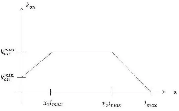
our application? Following [23], we chose to approximate kon by a function
Rezaei and J. Torrent, other choices like a Gaussian bell curve are also pos-sible, and we discuss this later). Thus with this parametrization we have 5
more parameterskmin
on , kmaxon , x1, x2, imax in addition to the 4 basic parameters
kI+, k−I , kN
on, kNof f to be estimated using our data sets.
Figure 2: Parametric representation for kon.
Thus we seek to estimate (withacceptable quantification of uncertainties)
the nine parameters kI+, k−
I , k
N
of f, kNon, and kon (represented in parametrical
form depicted above with the 5 additional unknowns kmin
on , kmaxon , x1, x2, imax)
that fit the data best! To do this we need an efficient discretization method
as discussed above for the forward problem as well as a correct assumption
on the measurement errors in the inverse problem.
3.1
Estimation of Parameters
We make some standard statistical assumptions (see [9, 10, 16, 26]) underly-ing our inverse problem formulations.
• Assume that there exists a true or nominal set of parameter θ0 =
(k−
I , ..., imax)
Denote the estimated parameter for θ0 as ˆθ. The inverse problem is based on statistical assumptions on the observation error in the data.
If we assume anabsolute error data modelthen data points are taken with
equal importance. This is represented by observations
yi =M(ti, θ0) +ǫi. (9)
On the other hand, if one assumes some type ofrelative error data model
then the error is proportional in some sense to the measured polymerized mass. This can be represented by observations of the form
yi =M(ti, θ0) +M(ti, θ0)γǫi, γ ∈(0,1]. (10)
Absolute model error formulations dictate we useOrdinary Least Squares
(OLS) inverse problem [9, 10] given by
ˆ
θ = arg minX(yi−M(ti, θ))2 (11)
while for relative error model one should use inverse problem formulations with Generalized Least Squares (GLS) cost functional
ˆ
θ= arg minX yi−M(ti, θ)
M(ti, θ)γ
2
, γ ∈(0,1]. (12)
3.1.1 The Residual Plots
To obtain a correct statistical model, we used residual plots (see [9, 10] for more details) with residuals given by
ri =
yi−M(ti,θˆ)
M(ti,θˆ)γ
, γ ∈[0,1]
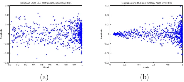
To illustrate what we are seeking for our data sets, we first used simulated
relative error data (simulated data for γ = 1), then carried out the inverse
problems for both a relative error cost functional (i.e.,γ = 1) and an ordinary
least squares cost functional (i.e.,γ = 0). We then plotted the corresponding
residuals vs time and also residuals vs the model values. The first plots are related to the correctness of our assumption of independency and identical
distributionsi.i.d. for the data whereas the second plots contain information
2 3 4 5 6 7 8 −0.03
−0.02 −0.01 0 0.01 0.02 0.03
Residuals using GLS cost function, noise level: 0.01
t
Residuals
1 2 3 4 5 6 7 8
−0.03 −0.02 −0.01 0 0.01 0.02 0.03
Residuals using OLS cost function, noise level: 0.01
t
Residuals
(a) (b)
Figure 3: Plots with simulated data: (a) Correct cost function vs. time
(γ = 1); (b)Incorrect cost function vs. time (γ = 0)
0.1 0.2 0.3 0.4 0.5 0.6 0.7 0.8 0.9 1 −0.03
−0.02 −0.01 0 0.01 0.02 0.03
Residuals using GLS cost function, noise level: 0.01
Model
Residuals
0 0.2 0.4 0.6 0.8 1 −0.03
−0.02 −0.01 0 0.01 0.02 0.03
Residuals using OLS cost function, noise level: 0.01
model
Residuals
(a) (b)
Figure 4: Plots with simulated data: (a) Correct cost function vs. model
3.2
Statistical Models of Noise
We next carried out similar inverse problems with data set (DS) 4 of our
experimental data collection. We first used DS 4 on the interval t ∈ [0,8].
Based on some earlier calculations we also chose the nucleation index i0 = 2
for all our subsequent calculations. The residual plots given below in Figures
5 and 6 suggest strongly that neitherof the first attempts of assumed
statis-tical models and corresponding cost functionals (absolute error and OLS or
relative error with γ = 1 and simple GLS) are correct.
0 1 2 3 4 5 6 7 8 9
0 0.1 0.2 0.3 0.4 0.5 0.6 0.7 0.8 0.9 1
time Madim for OLS and dataset 4
data Madim after opti
0 0.2 0.4 0.6 0.8 1
−8 −6 −4 −2 0 2 4 6 8x 10
−3 Residuals for OLS, N0=500 and dataset 4
model
Residuals
(a) (b)
Figure 5: (a) M(tk) with OLS; (b) Residuals vs Model: OLS
Based on these initial results and the speculation that early periods of the polymerization process may be somewhat stochastic in nature, we chose
to subsequently use all the data sets on the intervals [t0,8] where t0 is the
first time when M(t0) > 0.12 (thus 12% of the total polymerized mass).
Moreover, we decided to use other values of γ between 0 and 1 to test data
set 4.
We thus carried out further investigations with inverse problems for data
pointsM(tk)≥0.12 andi0 = 2 where we focused on the question of the most
appropriate values of γ to use in a generalized least squares approach (again
see [9] for further motivation and details). We then obtained the results with data set 4 depicted in Figure 7.
Analysis of these residuals suggest that either γ = 0.6 or γ = 0.7 might
0 1 2 3 4 5 6 7 8 9 0 0.1 0.2 0.3 0.4 0.5 0.6 0.7 0.8 0.9 1
Madim for GLS and dataset 4
data Madim after opti
0 0.2 0.4 0.6 0.8 1
−0.2 −0.15 −0.1 −0.05 0 0.05 0.1 0.15
Residuals vs model for GLS, N0=500 and dataset 4
Model
Residuals
(a) (b)
Figure 6: (a) M(tk) with GLS, γ = 1; (b) Residuals vs Model: GLS
0 0.2 0.4 0.6 0.8 1 −0.01 −0.005 0 0.005 0.01 gamma=0.0 model
0 0.2 0.4 0.6 0.8 1 −0.01 −0.005 0 0.005 0.01 gamma=0.1 model
0 0.2 0.4 0.6 0.8 1 −0.01 −0.005 0 0.005 0.01 gamma=0.2 model
0 0.2 0.4 0.6 0.8 1 −0.01 −0.005 0 0.005 0.01 gamma=0.3 model
0 0.2 0.4 0.6 0.8 1 −0.01 −0.005 0 0.005 0.01 gamma=0.4 model
0 0.2 0.4 0.6 0.8 1 −0.01 −0.005 0 0.005 0.01 gamma=0.5 model
0 0.2 0.4 0.6 0.8 1 −0.01 −0.005 0 0.005 0.01 gamma=0.6 model
0 0.2 0.4 0.6 0.8 1 −0.01 −0.005 0 0.005 0.01 gamma=0.7 model
0 0.2 0.4 0.6 0.8 1 −0.01 −0.005 0 0.005 0.01 gamma=0.8 model
0 0.2 0.4 0.6 0.8 1 −0.01 −0.005 0 0.005 0.01 gamma=0.9 model
0 0.2 0.4 0.6 0.8 1 −0.02 −0.01 0 0.01 0.02 gamma=1.0 model
Figure 7: Residuals for data set 4 using different values of γ.
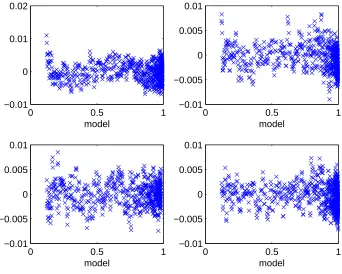
Motivated by these results, we next investigated the inverse problems
for each of the four experimental data sets with initial concentration c0 =
M(tk) ≥ 0.12 and used the generalized least squares method with γ = 0.6.
The resulting graphics depicted in Figure 8 again suggest that γ = 0.6 is a
reasonable value to use in our subsequent analysis of the polyglutamine data with regard to its information content for inverse problem estimation and parameter uncertainty quantification.
0 0.5 1
−0.01 0 0.01 0.02
model
0 0.5 1
−0.01 −0.005 0 0.005 0.01
model
0 0.5 1
−0.01 −0.005 0 0.005 0.01
model
0 0.5 1
−0.01 −0.005 0 0.005 0.01
model
4
Standard Errors and Asymptotic Analysis
4.1
Standard Errors for Parameters Using GLS
We employed first the asymptotic theory for parameter uncertainty summa-rized in [9, 10, 16] and the references therein. In the case of generalized least squares, the associated standard errors for the estimated parameters
ˆ
θ = (k+I , ..., imax) (vector lengthκθ = 9) are given by the following
construc-tion (for details see Chap. 3.2.5 and 3.2.6 of [9]): Define the covariance matrix by the formula
SEk =
q
Σkk(ˆθ), k = 1, ...,9,
where
Σ(ˆθ) = ˆσ2(χT(ˆθ)W(ˆθ)χ(ˆθ))−1.
Here χ is the sensitivity matrix of size n×κθ (n being the number of data
points and κθ being the number of estimated parameters) and W is defined
by
W−1(ˆθ) = diag(M(t1; ˆθ)2γ, . . . , M(tn; ˆθ)2γ).
We use the approximation of the variance
σ2 ≈σˆ(ˆθ)2 = 1
n−κθ n
X
i=1
1
M(ti; ˆθ)2γ
(M(ti,θˆ)−yi)2.
To obtain a finite standard error using asymptotic theory, the 9×9 matrix
F = χT(ˆθ)W(ˆθ)χ(ˆθ) thus must be invertible. In the above problem we do
indeed obtain a good fit of the curve and good residuals (for the sake of brevity, not depicted here!). However, we also found that the condition number of the matrix
F =χT(ˆθ)W(ˆθ)χ(ˆθ)
is κ = 1024. Looking more closely at the matrix F reveals a near linear
dependence between certain rows, hence the large condition number. We
thus quickly reach the following conclusions:
1. We obtain a set of parameters for which the model fits well, but we
2. We suspect that it may not be possible to obtain sufficient information from our data set curves to estimate all 9 parameters with a high degree of confidence! This is based on our calculations with the corresponding Fisher matrices as well our prior knowledge in that the graphs depicted in Figure 1 are very similar to Logistic or Gompertz curves which can be quite well fit with parameterized models with only 2 or 3 carefully chosen parameters!
To assist in initial understanding of these issues, we consider the associated
sensitivity matrices χ= ∂M
∂θ .
4.2
Sensitivity Analysis
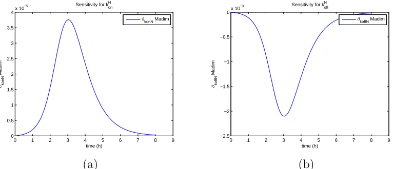
For the sensitivity analysis, we follow [9, 10]. Hereafter all our analysis will
be carried using data set 4 and the best estimate ˆθobtained for the latter. We
find that the model is sensitive mainly to four parameters: kI+, k−
I , konN, kNof f.
The sensitivities for the remaining parameters are on an order of magnitude
of 10−6 or less. It also shows some sensitivity with respect to x1. However,
the parameterx1appears in the model only as factorx1imax. The sensitivities
depicted below use ˆθ for the nine best fit GLS parameters , i.e., ˆθ for κθ = 9.
0 1 2 3 4 5 6 7 8 9 −0.1
−0.09 −0.08 −0.07 −0.06 −0.05 −0.04 −0.03 −0.02 −0.01 0
time (h)
∂kImoins
Madim
Sensitivity for kI −
∂kImoins Madim
0 1 2 3 4 5 6 7 8 9 0
0.1 0.2 0.3 0.4 0.5 0.6 0.7
time (h)
∂kIplus
Madim
Sensitivity for kI +
∂kIplus Madim
(a) (b)
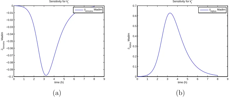
Figure 9: (a) Sensitivity w.r.t. k−
I ; (b) Sensitivity w.r.t. k
+
0 1 2 3 4 5 6 7 8 9 0 0.5 1 1.5 2 2.5 3 3.5
4x 10
−5
time (h)
∂konN
Madim
Sensitivity for konN
∂konN Madim
0 1 2 3 4 5 6 7 8 9 −2.5
−2 −1.5 −1 −0.5
0x 10
−3
time (h)
∂koffN
Madim
Sensitivity for koffN
∂koffN Madim
(a) (b)
Figure 10: (a) Sensitivity w.r.t. kN
on; (b) Sensitivity w.r.t. kof fN
0 1 2 3 4 5 6 7 8 9 0 0.2 0.4 0.6 0.8 1 1.2 1.4 1.6 1.8
2x 10
−6
time (h)
∂konmin
Madim
Sensitivity for kon min
∂konmin Madim
0 1 2 3 4 5 6 7 8 9 0 1 2 3 4 5 6 7 8x 10
−10
time (h)
∂konmax
Madim
Sensitivity for kon max
∂konmax Madim
(a) (b)
Figure 11: (a) Sensitivity w.r.t. kmin
0 1 2 3 4 5 6 7 8 9 −25
−20 −15 −10 −5 0
time (h)
∂x1
Madim
Sensitivity for x1
∂x1 Madim
0 1 2 3 4 5 6 7 8 9 0
0.5 1 1.5 2 2.5
3x 10
−59
time (h)
∂x2
Madim
Sensitivity for x2
∂x2 Madim
(a) (b)
Figure 12: (a) Sensitivity w.r.t. x1; (b) Sensitivity w.r.t. x2
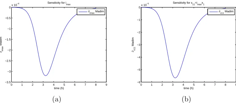
0 1 2 3 4 5 6 7 8 9 −3.5
−3 −2.5 −2 −1.5 −1 −0.5
0x 10
−6
time (h)
∂imax
Madim
Sensitivity for imax
∂imax Madim
0 1 2 3 4 5 6 7 8 9 −6
−5 −4 −3 −2 −1
0x 10
−5
time (h)
∂x11
Madim
Sensitivity for x11=imaxx1
∂x11 Madim
(a) (b)
5
Sensitivity Motivated Inverse Problems
Based on the sensitivity findings depicted above, we investigated a series of inverse problems in which we attempted to estimate an increasing number of
parameters beginning first with the fundamental parameters kI+ and kI−. In
each of these inverse problems we attempted to ascertain uncertainty bounds for the estimated parameters using both the asymptotic theory described above and a generalized least squares version of bootstrapping [12, 13, 15, 17, 19].
A quick outline of the appropriate bootstrapping algorithm is given next.
5.1
Bootstrapping Algorithm: Nonconstant Variance
Data
We suppose now that we are given experimental data (t1, y1), . . . ,(tn, yn)
from the underlying observation process
Yi =M(ti;θ0) +M(ti;θ0)γEei, (13)
wherei= 1, . . . , nand theEei arei.i.d. with mean zero and constant variance
σ02. Then we see that E(Yi) = M(ti;θ0) and V ar(Yi) = σ2
0M2γ(ti, θ0), with
associated corresponding realizations of Yi given by
yi =M(ti;θ0) +M(ti;θ0)γǫei.
A standard algorithm can be used to compute the corresponding
boot-strapping estimate θˆboot of θ0 and its empirical distribution. We treat the general case for nonlinear dependence of the model output on the
parame-ters θ. The algorithm is given as follows.
1. First obtain the estimate ˆθ0 from the entire sample{y
i}using the GLS
given in (12) withγ = 1. An estimate ˆθboot can be solved for iteratively
as follows.
2. Define the nonconstant variance standardized residuals
¯
si =
yi−M(t;θˆ0)
M(ti; ˆθ0)γ
, i= 1,2, . . . , n.
3. Create a bootstrapping sample of size n using random sampling with
replacement from the data (realizations) {s¯1,. . . ,¯sn} to form a
boot-strapping sample {sm
1 , . . . , smn}.
4. Create bootstrapping sample points
yim=M(ti; ˆθ0) +M(ti; ˆθ0)γsmi ,
where i= 1,. . . ,n.
5. Obtain a new estimate ˆθm+1 from the bootstrapping sample{yim}using
GLS.
6. Set m = m+ 1 and repeat steps 3–5 until m ≥ M where M is large
(e.g., M=1000).
We then calculate the mean, standard error, and confidence intervals using the formulae
ˆ
θboot = M1
PM
m=1θˆm,
Var(θboot) = M1−1PMm=1(ˆθm−θˆboot)T(ˆθm−θˆboot), (14)
SEk(ˆθboot) =
p
V ar(θboot)kk.
where θboot denotes the bootstrapping estimator.
5.2
Estimation of two parameters
We first carried out estimation for the 2 parameters kI+ and k−I . We use
the GLS formulation with γ = 0.6. We fix globally (based on previous
estimations with DS 4) the parameter values
konN kof fN k min
on kmaxon x1 x2 imax
4616.962 93.332 1684.381 1.5152·109 0.0626 0.859 3.542·105
and used the initial guesses for the parameters given by
kI+ k−
I
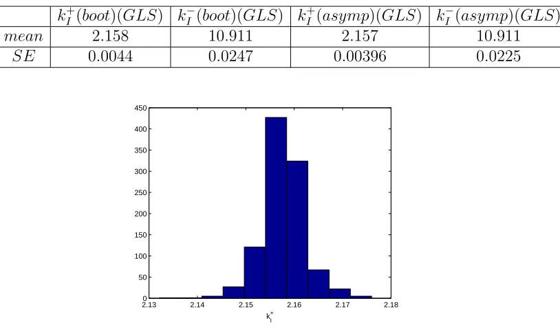
We then used the bootstrapping algorithm and obtained the following
means and standard errors for M = 1000 which, as reported below,
com-pare quite well with the asymptotic theory estimates. The corresponding distributions are shown in Figures 14 and 15.
kI+(boot)(GLS) k−
I (boot)(GLS) k
+
I (asymp)(GLS) k
−
I (asymp)(GLS)
mean 2.158 10.911 2.157 10.911
SE 0.0044 0.0247 0.00396 0.0225
2.130 2.14 2.15 2.16 2.17 2.18 50
100 150 200 250 300 350 400 450
k
I +
Figure 14: Two parameters estimation (k+I ,k−
I ). Bootstrapping distribution
for kI+. We use GLS and M=1000 runs.
5.3
GLS Estimation of 3 Parameters
We tried next to estimate 3 parameters. We again used the GLS formulation
with γ = 0.6. Once again we fixed all the parameters describing the domain
and the polymerization function kon and we also fixed either kNof f or konN in
the corresponding inverse problems.
5.4
GLS Estimation for
k
I+, k
I−and
k
NonWe fixed values as follows:
kof fN kminon konmax x1 x2 imax
10.750 10.8 10.85 10.9 10.95 11 11.05 11.1 50
100 150 200 250 300 350 400 450
k
I −
Figure 15: Two parameters estimation (k+I ,k−
I ). Bootstrapping distribution
for k−
I . We use GLS and M=1000 runs.
We used as initial parameter values:
k+I k−I konN
q0 2.1600 10.9270 4616.962
We obtained the estimated parameters together with the corresponding
stan-dard errors, variances and the condition numbers κ of the corresponding
sensitivity matrices for the four data sets as reported below. The 95% con-fidence results based on the asymptotic theory are also depicted for DS 4 in Figure 16.
kI+ k−
I kNon SE σ2 κ
DS1 2.26 13.49 4616.96 (.012, .099,53.925) 8.52·10−6 8.89·1010
DS2 2.99 16.20 4616.96 (.021, .151,56.691) 9.67·10−6 4.37·1010
DS3 2.18 15.76 9840.31 (.011, .103,90.466) 6.45·10−6 3.94·1011
DS4 2.16 10.91 4616.96 (0.0089,0.0649,45.262) 6.36·10−6 7.14·1010
To compare these asymptotic results with bootstrapping, we carried out
bootstrapping with Data Set (DS) 4 for the estimation ofk+I ,kI−andkN
onwith
the same initial values as above. We then obtained the following means and
1 2 3 4 2.2
2.4 2.6 2.8 3
data set
kI
+
95% confidence intervals for kI+
1 2 3 4
12 14 16
data set
kI
−
95% confidence intervals for kI−
1 2 3 4
4000 6000 8000 10000
data set
kon
N
95% confidence intervals for k
on N
Figure 16: Confidence Intervals
theory.
kI+(boot) k−
I (boot) k
N
on(boot) kI+(asymp) k
−
I (asymp) k N
on(asymp)
mean 2.153 10.887 4616.962 2.157 10.910 4616.962
SE 0.0039 0.0219 0.00003 0.0089 0.0649 45.262
Of particular interest are the values obtained forkN
on and the
bootstrap-ping standard errors for konN which are extremely small. It should be noted
that the sensitivity of the model output on kN
on is also very small. Thus one
might conjecture that the iterations in the bootstrapping algorithm do not
change the values of kN
on very much and hence one observes the extremely
10.80 10.82 10.84 10.86 10.88 10.9 10.92 10.94 10.96 10.98 50
100 150 200 250 300
Figure 17: Estimation for k+I ,k−
I andk
N
on: Bootstrapping distribution for k
−
I
for GLS and 1000 runs.
2.140 2.145 2.15 2.155 2.16 2.165 2.17 50
100 150 200 250
Figure 18: Estimation for k+I ,kI− andkN
on: Bootstrapping distribution for kI+
4616.9620 4616.962 4616.9621 4616.9621 4616.9622 4616.9622 4616.9623 50
100 150 200 250
Figure 19: Estimation fork+I ,kI−andkN
on: Bootstrapping distribution forkNon
5.5
GLS estimation for
k
I+, K
I−and
k
Nof fIn another test, we fixed kNon and instead estimate kNof f (along with kI+ and
k−
I ). We use the fixed values:
kN
on konmin kmaxon x1 x2 imax
4616.962 1684.381 1.5152·109 0.0626 0.859 3.542·105
and the initial guesses for the parameters to be estimated given by:
kI+ k−
I kof fN
q0 2.1600 10.9270 108.256
We obtained the estimated parameters and corresponding SE.
kI+ k−I kN
of f SE σ2 κ
DS1 2.203 12.997 99.861 (.011, .091,1.208) 8.165·10−6 4.912·107
DS2 2.893 15.474 100.019 (.019, .137,1.279) 9.323·10−6 2.486·107
DS3 2.168 15.631 41.935 (.011, .102,0.424) 6.435·10−6 9.125·106
DS4 2.181 11.090 90.536 (.009, .066,0.936) 6.289·10−6 3.043·107
Also in this case, we carried out bootstrapping for DS 4. The bootstrap-ping distributions for kI+, k−
I and kof fN are found in Figures 20-22. We then
obtained the following means and standard errors for a run with M = 1000
in comparison to the asymptotic theory.
kI+(boot) k−
I (boot) kof fN (boot) kI+(asymp) k
−
I (asymp) kof fN (asymp)
mean 2.169 11.013 91.254 2.181 11.090 90.536
2.140 2.15 2.16 2.17 2.18 2.19 2.2 2.21 50
100 150 200 250
k
I +
Figure 20: Three parameters estimation (kI+, k−
I and kof fN ): Bootstrapping
distribution for k+I . We used GLS and M=1000 runs.
10.80 10.9 11 11.1 11.2 11.3 50
100 150 200 250
k
I −
Figure 21: Three parameters estimation (kI+, k−
I and kof fN ): Bootstrapping
87 88 89 90 91 92 93 94 95 0
50 100 150 200 250
k
off N
Figure 22: Three parameters estimation (kI+, k−I and kof fN ): Bootstrapping
distribution for kN
5.6
Estimation of 4 main parameters
Following the sensitivity analysis detailed above, we tried to estimate a com-bination of the parametersk+I , kI−, kN
on, kNof f for the parameter set withκθ = 4.
Parameters as follows were fixed from the original 9 parameter fit:
kmin
on kmaxon x1 x2 imax
1684 1.5·109 0.062 0.859 3.5·105
We obtained the following result for the estimation of the four parameters using the data sets 1 to 4. In all of them, the condition number of the
Fischer’s information matrix κ is too large to invert. This along with the
sensitivity results above strongly suggests that the data sets do not contain sufficient information to estimate 4 or more parameters with any degree of certainty attached to the estimates.
k+I k−
I konN kof fN σ2 κ
DS1 2.1431 12.4751 4616.962 108.259 8.7219·10−6 6.1226·1019
DS2 2.7995 14.7630 4616.957 108.4308 9.8694·10−6 1.4442·1019
DS3 2.180 15.757 4618.599 41.369 6.4622·10−6 1.881·1017
DS4 2.161 10.9278 4617.3316 93.3265 6.374·10−6 2.144·1018
6
Model Comparison Tests
A type of Residuals Sum of Squares (RSS) based model selection criterion [8, 9, 10] can be used as a tool for model comparison for certain classes of models. In particular this is true for models such as those given in [3] in which potentially extraneous mechanisms can be eliminated from the model by a simple restriction on the underlying parameter space while the form of the mathematical model remains unchanged. In other words, this methodology can be used to compare two nested mathematical models where the parameter
set ΩH
θ (this notation will be defined explicitly in Section 6.1 below) for
the restricted model can be identified as a linearly restricted subset of the
admissible parameter set Ωθ of the unrestricted model. Indeed, the RSS
6.1
Ordinary Least Squares
We now turn to the statistical model (9), where the measurement errors are assumed to be independent and identically distributed with zero mean and
constant variance σ2. In addition, we assume that there exists θ
0 such that
the statistical model
Yj =M(tj;θ0) +Ej, j = 1,2, . . . , n. (15)
correctly describes the observation process. In other words, (15) is the true
model, and θ0 is the true value of the mathematical model parameterθ.
With our assumption on measurement errors, the mathematical model
parameter θ can be estimated by using the ordinary least squares method;
that is, the ordinary least squares estimator of θ is obtained by solving
θn = arg min
θ∈Ωθ
Jn(θ;Y).
Here Y= (Y1, Y2, . . . , Yn)T, and the cost function Jn is defined as
Jn(θ;Y) = 1
n
n
X
k=1
(Yk−M(tk;θ))2.
The corresponding realization ˆθn of θn is obtained by solving
ˆ
θn= arg min
θ∈Ωθ
Jn(θ;y),
where y is a realization of Y (that is, y= (y1, y2, . . . , yn)T).
As alluded to in the introduction, we might also consider a restricted version of the mathematical model in which the unknown true parameter
is assumed to lie in a subset ΩH
θ ⊂ Ωθ of the admissible parameter space.
We assume this restriction can be written as a linear constraint, Hθ0 = h,
where H ∈ Rκr×κq is a matrix having rank κ
r (that is, κr is the number of
constraints imposed), andhis a known vector. Thus the restricted parameter
space is
ΩH
θ ={θ ∈Ωθ :Hθ =h}.
Then the null and alternative hypotheses are
H0 : θ0 ∈ΩHθ
We may define the restricted parameter estimator as
θn,H = arg min
θ∈ΩH
θ
Jn(θ;Y),
and the corresponding realization is denoted by ˆθn,H. Since ΩH
θ ⊂ Ωθ, it is
clear that
Jn(ˆθn;y)≤Jn(ˆθn,H;y).
This fact forms the basis for a model selection criterion based upon the residual sum of squares. Using the standard assumptions (given in detail in
[9]), one can establish asymptotic convergence result for the test statistics
(which is a function of observations and is used to determine whether or not the null hypothesis is rejected)
Un= n J
n(θn,H;Y)−Jn(θn;Y)
Jn(θn;Y) ,
where the corresponding realization ˆUn is defined as
ˆ
Un=
nJn(ˆθn,H;y)−Jn(ˆθn;y)
Jn(ˆθn;y) . (16)
This asymptotic convergence result is summarized in the following theorem.
Theorem 6.1. Under assumptions detailed in [9, 10] and assuming the null hypothesis H0 is true, then Un converges in distribution (as n → ∞) to a
random variable U having a chi-square distribution with κr degrees of
free-dom.
The above theorem suggests that if the sample sizen is sufficiently large,
then Un is approximately chi-square distributed with κ
r degrees of freedom.
We use this fact to determine whether or not the null hypothesis H0 is
re-jected. To do that, we choose a significance level α (usually chosen to be
0.05) and useχ2 tables to obtain the correspondingthreshold valueτ so that
P rob(U > τ) = α. We next compute ˆUn and compare it to τ. If ˆUn > τ,
then we reject the null hypothesis H0 with confidence level (1 −α)100%;
otherwise, we do not reject. We emphasize that care should be taken in
confidence. The table below illustrates the threshold values for χ2(1) with the given significance level.
α τ conf idence level .25 1.32 75%
.1 2.71 90%
.05 3.84 95%
.01 6.63 99%
.001 10.83 99.9%
Similar tables can be found in any elementary statistics text or online or calculated by some software package such as Matlab, and is given here for illustrative purposes and also for use in the examples demonstrated below.
6.2
Generalized Least Squares
The model comparison results outlined can be extended to deal with gener-alized least squares problems in which measurement errors are independent with E(Ek) = 0 and V ar(Ek) =σ2w2(tk,θˆ), k = 1,2, . . . , n, where w is some
known real-valued function with w(t,θˆ) 6= 0 for any t. This is achieved
through rescaling the observations in accordance with their variance (as dis-cussed in [9]) so that the resulting (transformed) observations are identically distributed as well as independent.
6.3
Results for PolyQ Aggregation Models
We then carried out a series of model comparison tests (we again used DS 4) for nested models to determine if an added parameter yields a statistically
significantly improved model fit. Our null hypothesis in each case was: H0:
The restricted model is adequate (i.e., the fit-to-data is not significantly improved with the model containing the additional parameter as a parameter to be estimated). We obtained the following results.
1. Model with estimation of {k+I , k−
I } vs. the model with estimation
of {kI+, kI−, kN
of f} : We find with n=699, Jn(ˆθnH;Y) = .0044192109,
Jn(ˆθn;Y) = .0043709501 and ˆUn = 7.7178. Thus we reject H0 at a
2. Model with estimation of {kI+, kI−} vs. the model with estimation of
{kI+, k−
I , k
N
on} : We find Jn(ˆθn;Y) = .0044192108 with ˆUn = 7.49×
10−06. Thus we don’t rejectH
0 at a 99% confidence level.
3. Model with estimation of{kI+, k−I , kNof f}vs. the model with estimation
of{k+I , k−
I , kof fN , kNon}: To the order of computation we find no difference
in the cost functions in this case and therefore we do not reject H0 at
a confidence level of 99%.
4. Model with estimation of{kI+, k−
I , kNon}vs. the model with estimation of
{kI+, k−I , kNon, kof fN }: We findJn(ˆθn;Y) =.0043709780 with ˆUn = 7.7133
and hence we reject H0 with a confidence level of 99%.
From these and the preceding results we conclude the information content of the typical data set for the dynamics considered here will support at most 3 parameters estimated with reasonable confidence levels and these are the parameters {kI+, kI−, kN
of f}.
7
Conclusions and Suggested Further Efforts
For the efforts reported on above we make several conclusions.
For the majority of data sets, the GLS residual plots with γ = 0.6 are
random when fitted for data points M(tk) ≥ 0.12. As conjectured earlier,
this may be because the early formation of aggregates is somewhat stochas-tic in nature which is not well described by either the mathemastochas-tical and/or statistical models. It appears that one needs special consideration of smaller polymer sizes. Indeed we suspect from additional discussions with our col-leagues that perhaps the nucleation step might be dominated by a stochastic rather than deterministic process in the early stages (i.e., for small polymer sizes). This is a possible direction of further investigation.
Based on several different mathematical/statistical methodologies (sen-sitivities, asymptotic analysis, bootstrapping, model comparison tests), the data sets we considered do not contain sufficient information for the reliable estimation of all 9 parameters of interest. Indeed our findings suggest that at most 3 parameters can be reliably estimated with the data sets typical
of those presented here, and that these parameters are {kI+, k−
I , kNof f}.
more sophisticated models derived in [23], especially in order to investigate information coming from different initial concentrations. Indeed, we have considered here data sets related to experiments carried out with the same
initial concentration. Adapting the previously used techniques to
simulta-neously or successively use all the information content in data sets carried out for different initial concentration is a challenging problem (see [22] for a discussion of the effect of initial concentration on nucleated polymerization). Here we conclude that at most 3 parameters{kI+, kI−, kNof f}can be reliably estimated with the data sets investigated. The two first parameters determine the balance between the normal and abnormal protein concentrations and the third represents the stability of the nucleus against the degradation into monomeric entities. These three parameters are related to the early steps of the aggregation process, and thus we conclude that the model applied to these data sets does not provide any insight into the polymerization of larger polymers. Since this is the case, there is little motivation to modify the polymerization function depicted in Figure 2 until further data collection procedures are pursued.
Acknowledgements
This research was supported in part (MD, CK) by the ERC Starting Grant SKIPPERAD, in part (HTB) by Grant Number NIAID R01AI071915-10 from the National Institute of Allergy and Infectious Diseases, and in part (HTB) by the Air Force Office of Scientific Research under grant number AFOSR FA9550-12-1-0188.
References
[1] B.M. Adams, H.T. Banks, M. Davidian, and E.S. Rosenberg, Model fitting and prediction with HIV treatment interruption data, Center for Research in Scientific Computation Technical Report CRSC-TR05-40,
NC State Univ., October, 2005; Bulletin of Math. Biology, 69 (2007),
563–584.
CRSC-TR14-12, N. C. State University, Raleigh, NC, September, 2014;Applied Mathematics Letters,40 (2015), 84–89; DOI: 10.1016/j.aml.2014.09.013.
[3] H.T. Banks, J.E. Banks, K. Link, J.A. Rosenheim, Chelsea Ross, and K.A. Tillman, Model comparison tests to determine data information content, CRSC-TR14-13, N. C. State University, Raleigh, NC, October,
2014;Applied Math Letters, to appear.
[4] H.T. Banks, R. Baraldi, K. Cross, K. Flores, C. McChesney, L. Poag, and E. Thorpe, Uncertainty quantification in modeling HIV viral mechanics, CRSC-TR13-16, N. C. State University, Raleigh, NC, December, 2013;
Math. Biosciences and Engr., submitted.
[5] H.T. Banks, A. Cintron-Arias and F. Kappel, Parameter selection meth-ods in inverse problem formulation, CRSC-TR10-03, N.C. State
Univer-sity, February, 2010, Revised, November, 2010; inMathematical Modeling
and Validation in Physiology: Application to the Cardiovascular and Res-piratory Systems,(J. J. Batzel, M. Bachar, and F. Kappel, eds.), pp. 43 – 73, Lecture Notes in Mathematics Vol. 2064, Springer-Verlag, Berlin 2013.
[6] H. T. Banks, M. Davidian, S. Hu, G. M. Kepler, and E. S. Rosenberg,
Modeling HIV immune response and validation with clinical data,Journal
of Biological Dynamics,2 (2008), 357–385.
[7] H.T. Banks, M. Doumic and C. Kruse, Efficient numerical schemes for Nucleation-Aggregation models: Early steps, CRSC-TR14-01, N. C. State University, Raleigh, NC, March, 2014.
[8] H.T. Banks and B.G. Fitzpatrick, Statistical methods for model
compar-ison in parameter estimation problems for distributed systems, Journal
of Mathematical Biology, 28 (1990), 501-527.
[9] H.T. Banks, S. Hu and W.C. Thompson, Modeling and Inverse
Prob-lems in the Presence of Uncertainty, Taylor/Francis-Chapman/Hall-CRC Press, Boca Raton, FL, 2014.
[10] H.T. Banks and H.T. Tran, Mathematical and Experimental Modeling
[11] V. Calvez and N. Lenuzza and M. Doumic and J.-P. Deslys and F.
Mouthon and B. Perthame, Prion dynamic with size dependency - strain
phenomena, J. of Biol. Dyn., 4 (1), 28–42.
[12] R.J. Carroll and D. Ruppert, Transformation and Weighting in
Regres-sion,Chapman & Hall, New York, 1988.
[13] R.J. Carroll, C.F.J. Wu and D. Ruppert, The effect of estimating weights
in Weighted Least Squares, J. Amer. Statistical Assoc., 83(1988), 1045–
1054.
[14] J.F. Collet, T. Goudon,F. Poupaud and A. Vasseur, The Becker-D¨oring
system and its Lifshitz-Slyozov limit, SIAM J. Appl. Math., 62 (2002),
1488–1500.
[15] M. Davidian, Nonlinear Models for Univariate and Multivariate
Re-sponse, ST 762 Lecture Notes, Chapters 2, 3, 9 and 11, 2007; http://www4.stat.ncsu.edu/ davidian/courses.html
[16] M. Davidian and D.M. Giltinan, Nonlinear Models for Repeated
Mea-surement Data, Chapman and Hall, London, 2000.
[17] T.J. DiCiccio and B. Efron, Bootstrap confidence intervals, Statistical
Science, 11 (1995), 189–228.
[18] M. Doumic, T. Goudon and T. Lepoutre, Scaling limit of a discrete
prion dynamics model,Commun. Math. Sci., 7 (2009), 839–865.
[19] B. Efron, The Jackknife, the Bootstrap and Other Resampling Plans,
CBMS 38, SIAM Publishing, Philadelphia, PA, 1982.
[20] P. Lauren¸cot and S. Mischler, From the discrete to the continuous
coagu-lationfragmentation equations,Proc. Royal Society of Edinburgh: Section
A Mathematics, 132 (2002), 1219–1248.
[21] R.J. LeVeque, Finite-Volume Methods for Hyperbolic Problems,
Cam-bridge University Press, 2002.
[22] E.T. Powers and D.L. Powers, The kinetics of nucleated polymeriza-tions at high concentrapolymeriza-tions: Amyloid fibril formation near and above
[23] S. Prigent, A. Ballesta, F. Charles, N. Lenuzza, P. Gabriel, L.M. Tine, H. Rezaei and M. Doumic, An efficient kinetic model for assemblies of
amyloid fibrils and its application to polyglutamine aggregation, PLoS
ONE, 7 (2012), e43273; DOI:10.1371/journal.pone.0043273
[24] F. Eghiaian, T. Daubenfeld, Y. Quenet, M. van Audenhaege, A.P. Bouin, G. van der Rest, J. Grosclaude and H. Rezaei, Diversity in prion protein oligomerization pathways results from domain expansion as
re-vealed by hydrogen/deuterium exchange and disulfide linkage, PNAS, bf
104 (18), 2007, 7414–7419.
[25] S.I. Rubinow,Introduction to Mathematical Biology, John Wiley & Sons,
New York, 1975.
[26] G.A.F. Seber and C.J. Wild, Nonlinear Regression, J. Wiley & Sons,
Hoboken, NJ, 2003.
[27] Wei-Feng Xue, S.W. Homans and S.E. Radford, Systematic analysis of nucleation-dependent polymerization reveals new insights into the
mech-anism of amyloid self-assembly, Proc Natl Acad Sci U S A, 105 (2008),
8926–8931.
[28] W.-F. Xue, S. W. Homans, and S. E. Radford, Amyloid fibril length distribution quantified by atomic force microscopy single-particle image
analysis,Protein Engineering, Design & Selection:PEDS,22(2009),489–
496.
[29] W.-F. Xue and S. E. Radford, An imaging and systems modeling
ap-proach to fibril breakage enables prediction of amyloid behavior,
![Figure 1: The data sets of interest from [23, 7].](https://thumb-us.123doks.com/thumbv2/123dok_us/1516175.1185762/3.612.173.445.337.551/figure-data-sets.webp)